Implications of Coupling in Quantum Thermodynamic Machines

Abstract

We study coupled quantum systems as the working media of thermodynamic machines. Under a suitable phase-space transformation, the coupled systems can be expressed as a composition of independent subsystems. We find that for the coupled systems, the figures of merit, that is the efficiency for engine and the coefficient of performance for refrigerator, are bounded (both from above and from below) by the corresponding figures of merit of the independent subsystems. We also show that the optimum work extractable from a coupled system is upper bounded by the optimum work obtained from the uncoupled system, thereby showing that the quantum correlations do not help in optimal work extraction. Further, we study two explicit examples; coupled spin-$1/2$ systems and coupled quantum oscillators with analogous interactions. Interestingly, for particular kind of interactions, the efficiency of the coupled oscillators outperforms that of the coupled spin-$1/2$ systems when they work as heat engines. However, for the same interaction, the coefficient of performance behaves in a reverse manner, while the systems work as the refrigerator. Thus, the same coupling can cause opposite effects in the figures of merit of heat engine and refrigerator.

1. Introduction

Study of thermodynamics in quantum regime can reveal new aspects of fundamental interests. As an example, the statement of the second law of thermodynamics in the presence of an ancilla [1,2] or, when the system has coherence [3,4], has been established in great details, from where the classical version of the second law emerges under appropriate limits. The study of thermodynamics in quantum domain can be approached from different directions such as information-theoretic point of view [5,6,7,8,9,10] or resource-theoretic aspect [11,12,13]. Another important constituent, in this area of study, is the work extraction from quantum systems [14,15,16,17,18]. Besides these, analyzing different models of thermodynamic machines in the quantum domain can also provide new insight. Such a study helps us to understand the special behavior of thermodynamic quantities like work, heat, and efficiency in the quantum regime due to the presence non-classical features such as entanglement, quantum superposition, squeezing, etc. [19,20,21]. The quantum heat devices can show interesting atypical behaviors such as exceeding Carnot limit [19,21] when they act as heat engines. However, these apparent behaviors are found to be compatible with the second law of thermodynamics when all the preparation costs are considered [22]. Such machines also have practical importance in the realm of quantum computation and refrigeration of small systems [23].

The performance of coupled quantum systems as heat engines have been studied widely in recent past [24,25,26,27,28,29,30]. Work and efficiency are two important quantities to characterize the performance of a heat engine. It has been shown that appropriate coupling can increase the efficiency of the system compared to the uncoupled one [27]. In this work, we find an upper as well as a lower bound of the efficiency of the coupled system. We also show that the coupling and quantum correlations give no advantage to obtain optimum work when the working medium consists of quantum systems with quadratic coupling (to be specified later). The generality of these results are shown by considering different heat cycles.

Further, we compare the performances of different coupled quantum systems when used as the working medium of a heat device. For this purpose, we consider two extreme cases: coupled spin-$1/2$ systems (finite dimension) and coupled quantum oscillators (infinite dimension) as the working media of heat devices. In the case of Otto cycle, when there is no coupling, both the system has the same efficiency but the work output is higher for oscillator model. To compare the performance of the coupled systems, an analogous coupling for both the systems is taken. We consider that two spin-$1/2$ systems are coupled via Heisenberg XX or XY model of interaction [31,32]. For harmonic oscillators, we take quadratic interaction in both positions and momenta, which is analogous to the Heisenberg exchange interaction in spin systems. For this interaction, the Hamiltonians for coupled spins and coupled oscillators are similar in terms of ladder operators. The similar form of the free Hamiltonians for both of the systems is also ensured.

Here it is important to note that very recently, the performance of coupled harmonic oscillators as a heat engine is studied [30]. But, in contrast to the present work, there the interaction has been considered only between the position degrees of freedom of two oscillators. Furthermore, the authors in [30] have done the efficiency analysis for two different modes separately. But, the actual efficiency of the system has to be defined by the ratio of total work (done by both the modes) to the total heat which we analyze here. Therefore, our analysis provides a comprehensive picture of the efficiency of the coupled system. The main results of our work are as follows:

(i)

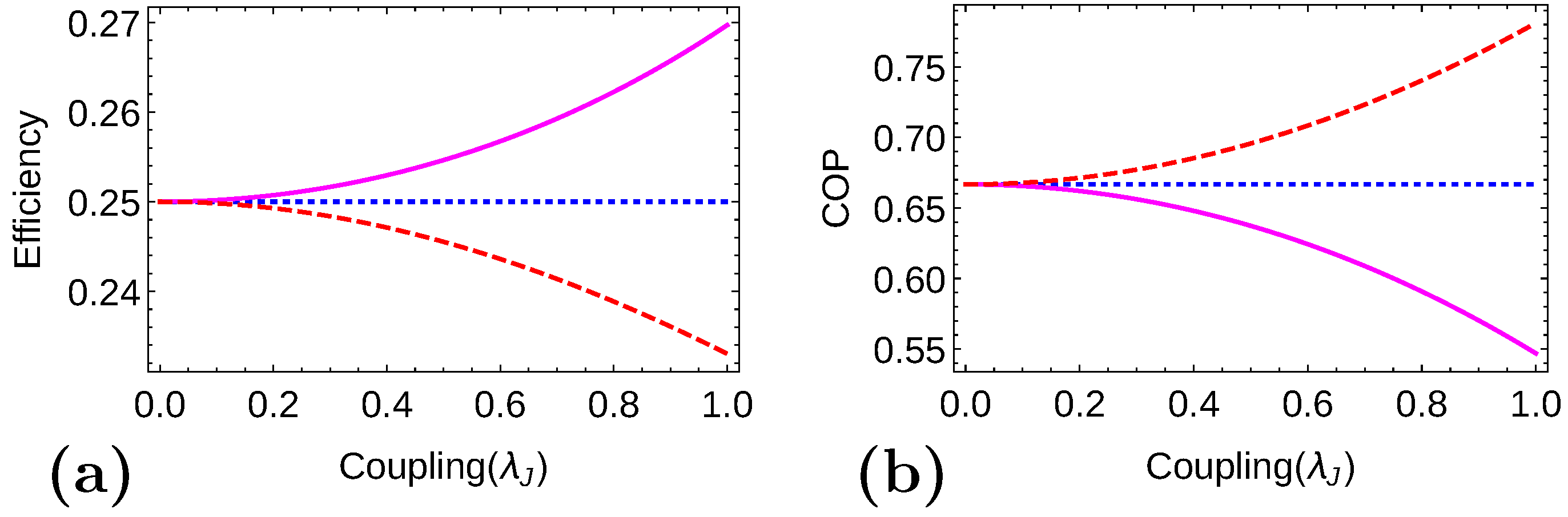
When the Hamiltonian of the coupled system (at all stages of the cycle) can be decoupled (as two independent modes) in some suitably chosen co-ordinate system, then the efficiency of the coupled system is bounded (both from above and below) by the efficiencies of the independent modes, provided both the modes work as engines (Section 3.1).

(ii)

The global efficiency (i.e., efficiency of coupled system) reaches the lower bound (mentioned in (i)) when the upper bound (mentioned in (i)) of the efficiency achieves Carnot efficiency. When one of the modes is not working as an engine, the global efficiency is upper bounded by the efficiency of the other mode (Section 4.1).

(iii)

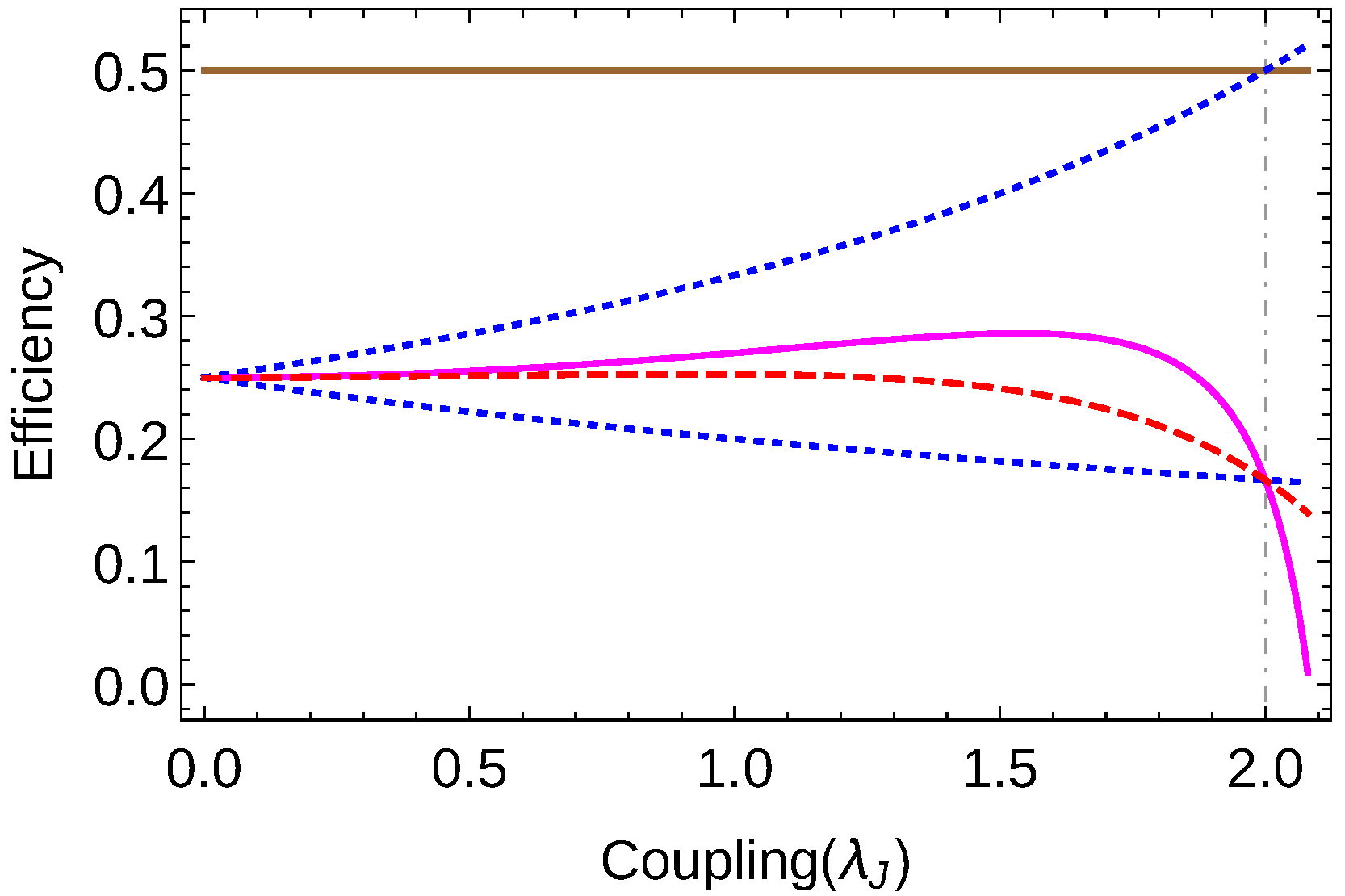
For the case of the engine, we compare the efficiencies in two extreme cases (coupled oscillators and coupled spin-$1/2$ systems). Interestingly, the efficiency of coupled oscillators outperforms the efficiency obtained from coupled spins (Section 4.1 and Section 4.3).

(iv)

We have also shown that the optimal work extractable from a coupled system is upper bounded by the optimal work extractable from the uncoupled systems (Section 3.3).

For meticulous comparison, we also consider coupled oscillators and coupled spins as the working medium of a refrigerator. The refrigeration cycle is similar to that of the heat engine. We find that:

(v)

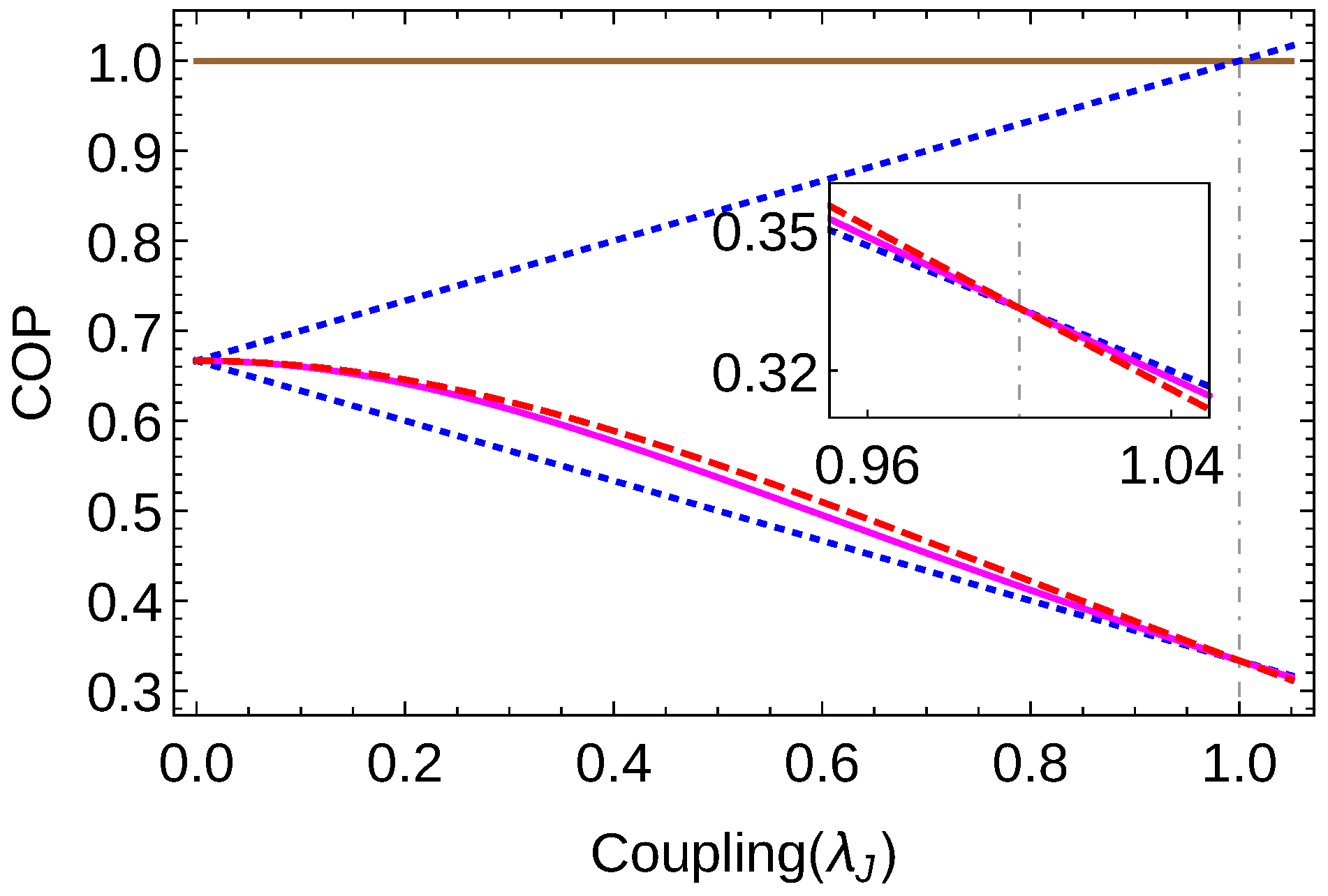
Like the efficiency, the global coefficient of performance (COP) is bounded (both from above and below) by the COPs of the independent modes (Section 5).

(vi)

Surprisingly, for similar interactions considered in the case of heat engine, the global COP of coupled spins is higher than that of the coupled oscillators, which is contrary to the behavior observed in the case of engines (Section 5.1 and Section 5.2).

Organization of the paper goes as follows: In Section 2, we introduce the Otto cycle and illustrate the performance of uncoupled spins and oscillators as the working substance. In Section 3, a general form of quadratic coupling in harmonic oscillators and their characteristics are discussed when they work as a heat engine. Further, we discuss similar forms of coupling found in spin systems, widely known as Heisenberg XY model. In Section 4, we describe the performance of the engine for special cases. Performances of the systems as refrigerators is discussed in Section 5. Section 6 is devoted to discussions and future possibilities.

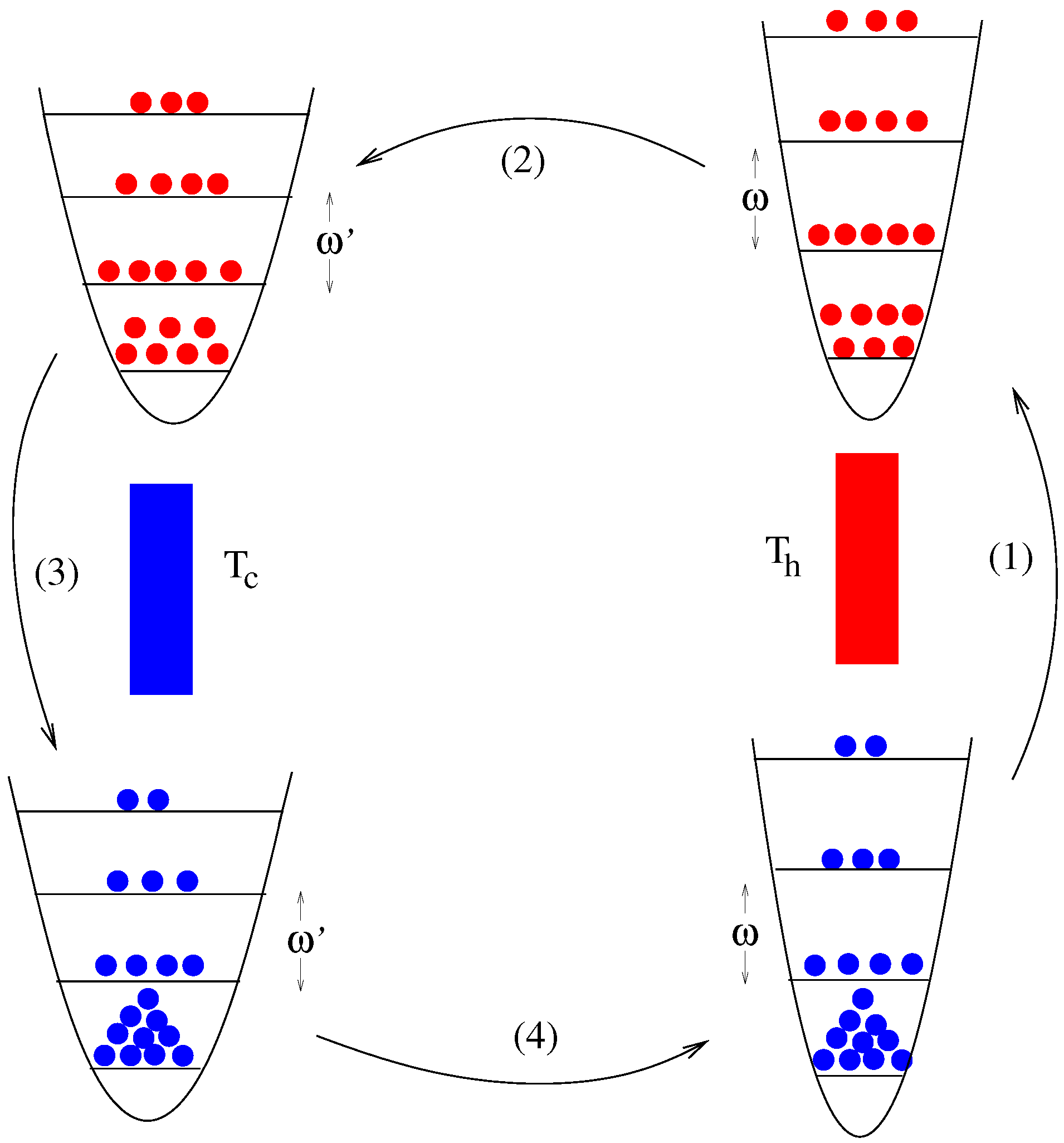
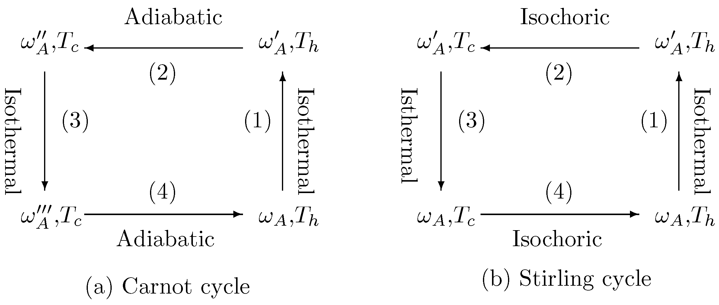
2. Quantum Otto Cycle

Quantum Otto cycles are analogous to the classical Otto cycle, and the latter consists of two isochoric processes (work, $W=0$) and two adiabatic processes (heat, $Q=0$). When the working medium of the Otto cycle is classical ideal gas, the efficiency of the system is written as $\eta =1-{(V_1/V_2)}^{\gamma -1}$, where $V_1$ and $V_2$ are initial and final volumes ($V_1<V_2$) of the adiabatic expansion process and $\gamma =C_p/C_v$, is the ratio of the specific heats [33]. Similar to the classical cycle, the quantum Otto cycle consists of two adiabatic processes and two thermalization processes [34,35]. The system exchanges heat with the bath during the thermalization processes and the work is done when the system undergoes adiabatic processes. Work and heat are calculated from the change in mean energies, where mean energy, for a system represented by the state $\rho$ and the Hamiltonian H, is defined as $\mathrm{Tr}\left[\rho H\right]$.

Here, we consider a four-staged Otto cycle. As an example, harmonic oscillator as the working medium of a quantum Otto cycle is pictorially described in Figure 1. The four stages of the cycle are:

Stage 1: 

In this stage, the system represented by the density matrix ${\rho }_c^{\prime }$ (defined in Stage 4) and the Hamiltonian H, is attached to a hot bath at temperature $T_h$. During the process, the Hamiltonian is kept fixed. At the end of this stage, the system reaches equilibrium with the bath. Therefore, the final state is given as ${\rho }_h=exp(-{\beta }_{h}H)/\mathrm{Tr}[exp(-{\beta }_{h}H)]$, where ${\beta }_h=1/k_B{T}_h$, with $k_B$ being the Boltzmann constant. Hence the amount of heat absorbed by the system from the hot bath is $Q_h=\mathrm{Tr}\left[H({\rho }_h-{\rho }_c^{\prime })\right]$.

Stage 2: 

The system is decoupled from the bath and the Hamiltonian is changed from H to $H^{\prime }$ slowly enough so that the quantum adiabatic theorem holds. Since there is no heat exchange between the system and the bath, the change in mean energy is equal to the work. The work done in this process is $w_1=\mathrm{Tr}\left[({\rho }_{h}H-{\rho }_h^{\prime }{H}^{\prime })\right]$, where ${\rho }_h^{\prime }=U_I{\rho }_h{U}_I^{†}$ and $U_I$ is the unitary associated with the adiabatic process, defined as $U_I=\mathcal{T}exp[-(i/\hslash ){\int }_0^{\tau }H\left(t\right)dt]$. Here $\mathcal{T}$ is the time ordering operator, $H\left(0\right)=H$ and $H\left(\tau \right)=H^{\prime }$.

Stage 3: 

The system is attached to the cold bath at inverse temperature ${\beta }_c=1/k_B{T}_c$. The system reaches equilibrium with the cold bath at the end of the process and the state of the system becomes ${\rho }_c=exp(-{\beta }_c{H}^{\prime })/\mathrm{Tr}[exp(-{\beta }_c{H}^{\prime })]$. Therefore the heat rejected to the cold bath is given as $Q_c=\mathrm{Tr}\left[H^{\prime }({\rho }_c-{\rho }_h^{\prime })\right]$.

Stage 4: 

The system is detached from the cold bath and the Hamiltonian is slowly varied from $H^{\prime }$ to H. The work done in this process is equal to the change in the mean energy, which is given as $w_2=\mathrm{Tr}\left[({\rho }_c{H}^{\prime }-{\rho }_c^{\prime }H)\right]$, where ${\rho }_c^{\prime }$ is the density matrix at the end of the adiabatic process, defined as ${\rho }_c^{\prime }=U_{II}{\rho }_c{U}_{II}^{†}$ and $U_{II}$ is given by $U_{II}=\mathcal{T}exp[-(i/\hslash ){\int }_0^{\tau }H\left(t\right)dt]$, so that $H\left(0\right)=H^{\prime }$ and $H\left(\tau \right)=H$. Finally, the cycle is completed by attaching the system with the hot bath.

The net work done by the system is $W=w_1+w_2=Q_h+Q_c$ and the efficiency is defined as $\eta =W/Q_h$.

In references [36,37], a two-staged cycle is considered with two n-level systems. There, the coupling between two n-level systems is only for a short time to perform SWAP like operations. This cycle is equivalent to a cycle with single n-level system undergoing a four-staged Otto cycle. This type of cycle is considered in Section 2.1. Our cycle is a four staged cycle, where the working medium consists of two oscillators (or spins) coupled to each other throughout the cycle. Both the subsystems are connected to one and the same bath at a time. Our primary aim is to find the effect of this coupling in the performance of the engine or refrigerator. We analyze the performance of the system using internal parameters such as bare mode frequencies and coupling strengths. Later in this paper, we consider mean energy preserving co-ordinate transformations. We refer the subsystems after the co-ordinate transformations as “independent subsystems” since they appear to be independent but they may not represent the actual subsystems. Before discussing the coupled systems, we briefly review the case of a single system as a heat engine.

2.1. Single System as a Heat Engine

Otto cycle with a single harmonic oscillator (or a spin system) constituting the working medium of the engine is studied in different works [27,30,34,35,38,39]. Here we briefly review this. Consider a harmonic oscillator with Hamiltonian

$$H^{\mathrm{os}}=\frac{p^2}{2m}+\frac{m{\mathsf{\Omega }}^2}{2}{x}^2=\left(c^{†}c+\frac{1}{2}\right)\mathsf{\Omega },$$

(1)

where m is the mass and $\mathsf{\Omega }$ is the frequency of the oscillator, and $c^{†}=x\sqrt{m\mathsf{\Omega }/2}-ip/\sqrt{2m\mathsf{\Omega }}$ and $c=x\sqrt{m\mathsf{\Omega }/2}+ip/\sqrt{2m\mathsf{\Omega }}$ are the creation and the annihilation operators respectively. We set ℏ and $k_B$ to unity. The cycle is constructed such that in Stage 2, the frequency is changed from $\mathsf{\Omega }=\omega$ to $\mathsf{\Omega }={\omega }^{\prime }$ and in Stage 4, ${\omega }^{\prime }$ is changed to $\omega$. In Stages 1 and 3, thermalization occurs with the respective heat baths as discussed above. The mean population of the thermal state of a harmonic oscillator with frequency $\mathsf{\Omega }$ and inverse temperature $\beta$ is $\langle c^{†}c\rangle =\langle n\rangle =1/(exp\beta \mathsf{\Omega }-1)$. We also assume that the adiabatic processes are slow enough ($\tau \to \infty$ in Stages 2 and 4), so that coherence is not created between the eigenstates of the final Hamiltonian. Therefore, the mean population in the initial and the final states of the adiabatic process are same. Under these assumptions, the heat absorbed from hot reservoir is given by

$$\begin{array}{cc}\hfill Q_h^{\mathrm{os}}& =\mathrm{Tr}\left[H^{\mathrm{os}}({\rho }_h-{\rho }_c^{\prime })\right]\hfill \\ \hfill & =\frac{\omega }{2}\left(\coth \left[\frac{{\beta }_h\omega }{2}\right]-coth\left[\frac{{\beta }_c{\omega }^{\prime }}{2}\right]\right),\hfill \end{array}$$

(2)

where $H^{\mathrm{os}}$ is obtained by substituting $\mathsf{\Omega }=\omega$ in Equation (1). Here ${\rho }_c^{\prime }$ and ${\rho }_h$ are respectively the initial and the final density matrices in Stage 1. Similarly, the heat rejected to the cold reservoir is

$$\begin{array}{cc}\hfill Q_c^{\mathrm{os}}& =\mathrm{Tr}\left[H^{\prime \mathrm{os}}({\rho }_c-{\rho }_h^{\prime })\right]\hfill \\ \hfill & =-\frac{{\omega }^{\prime }}{2}\left(\coth \left[\frac{{\beta }_h\omega }{2}\right]-coth\left[\frac{{\beta }_c{\omega }^{\prime }}{2}\right]\right),\hfill \end{array}$$

(3)

where $H^{\prime \mathrm{os}}$ is calculated by substituting $\mathsf{\Omega }={\omega }^{\prime }$ in Equation (1) and ${\rho }_h^{\prime }$ and ${\rho }_c$ are the initial and final density matrices respectively for the thermalization process described in Stage 3. The net work done by the system is given as $W^{\mathrm{os}}=Q_h^{\mathrm{os}}+Q_c^{\mathrm{os}}$:

$$W^{\mathrm{os}}=\frac{(\omega -{\omega }^{\prime })}{2}\left(\coth \left[\frac{{\beta }_h\omega }{2}\right]-coth\left[\frac{{\beta }_c{\omega }^{\prime }}{2}\right]\right).$$

(4)

The efficiency of the system is then given as

$${\eta }^{\mathrm{os}}\equiv \frac{W^{\mathrm{os}}}{Q_h^{\mathrm{os}}}=1-\frac{{\omega }^{\prime }}{\omega }.$$

(5)

The condition for the system to work as an engine is $W^{\mathrm{os}}\ge 0$ (with $Q_h^{\mathrm{os}}\ge 0$) is satisfied when ${\beta }_h\omega \le {\beta }_c{\omega }^{\prime }$ and $\omega >{\omega }^{\prime }$, so that we have ${\eta }^{\mathrm{os}}\le 1-{\beta }_h/{\beta }_c={\eta }_c$, where ${\eta }_c$ is the Carnot efficiency. The work output is zero when the system operates at Carnot value.

Now, consider a single spin-$1/2$ system, placed under a magnetic field $B_z$ applied along the z-direction. To get a similar form like oscillator, we need to add a term of the form $\mu B_z{I}_2$, where $I_2$ is the identity matrix and $\mu$ is a constant. Adding a constant term ($\mu B_z$) with each energy eigenvalue does not alter the characteristics of the engine. Thus we can write the corresponding Hamiltonian as,

$$H^{\mathrm{sp}}=\mu B_z(S_z+I)=\left(S^{+}{S}^{-}+\frac{1}{2}\right)\mathsf{\Omega },$$

(6)

where $S_z={\sigma }_z/2$, $\mathsf{\Omega }=\mu B_z$ and $S^{+}$ and $S^{-}$ are raising and lowering operators respectively. This Hamiltonian has a similar structure as the oscillator Hamiltonian given in Equation (1). Now consider a cycle constructed such that frequency $\mathsf{\Omega }$ varies from $\omega$ to ${\omega }^{\prime }$ in Stage 2 and returns to the initial value (${\omega }^{\prime }\to \omega$) in Stage 4. The heat absorbed from the hot reservoir is

$$\begin{array}{cc}\hfill Q_h^{\mathrm{sp}}& =\mathrm{Tr}\left[H^{\mathrm{sp}}({\rho }_h-{\rho }_c^{\prime })\right]\hfill \\ \hfill & =\frac{\omega }{2}\left(tanh\left[\frac{{\beta }_c{\omega }^{\prime }}{2}\right]-tanh\left[\frac{{\beta }_h\omega }{2}\right]\right),\hfill \end{array}$$

(7)

where $H^{\mathrm{sp}}$ is obtained by substituting $\mathsf{\Omega }=\omega$ in Equation (6). We also have ${\rho }_c^{\prime }={\rho }_c$ and ${\rho }_h^{\prime }={\rho }_h$, since $[U_{II},{\rho }_c]=0$ in Stage 4 and $[U_I,{\rho }_h]=0$ in Stage 2. Similar as above, the net work done by the system is given by

$$W^{\mathrm{sp}}=\frac{(\omega -{\omega }^{\prime })}{2}\left(tanh\left[\frac{{\beta }_c{\omega }^{\prime }}{2}\right]-tanh\left[\frac{{\beta }_h\omega }{2}\right]\right).$$

(8)

So we can calculate the efficiency of system as

$${\eta }^{\mathrm{sp}}=\frac{W^{\mathrm{sp}}}{Q_h^{\mathrm{sp}}}=1-\frac{{\omega }^{\prime }}{\omega }.$$

(9)

Even though the dimensionality of spin and harmonic oscillators are different, we kept the same energy level spacings in both the cases. Hence, both the cycles have the same efficiencies as shown in Equations (5) and (9). From Equations (4) and (8), we have $W^{\mathrm{os}}\ge W^{\mathrm{sp}}$. This inequality is true, because, for positive real values of x and y ($x\equiv {\beta }_h\omega /2<y\equiv {\beta }_c{\omega }^{\prime }/2$), we have $(coth\left[x\right]-coth\left[y\right])\ge (tanh\left[y\right]-tanh\left[x\right])$.

Consider two single systems (oscillators or spins), which are uncoupled and undergoing the cycle as discussed above. Then the work done by uncoupled oscillators is $2W^{\mathrm{os}}$ is greater than the work done by the spins $2W^{\mathrm{sp}}$. However, the efficiency of the uncoupled oscillators is equal to that of uncoupled spins, ${\eta }^{\mathrm{os}}={\eta }^{\mathrm{sp}}=1-{\omega }^{\prime }/\omega$. Now, our interest is to compare the performances of spins and oscillators when the analogous type of coupling is introduced.

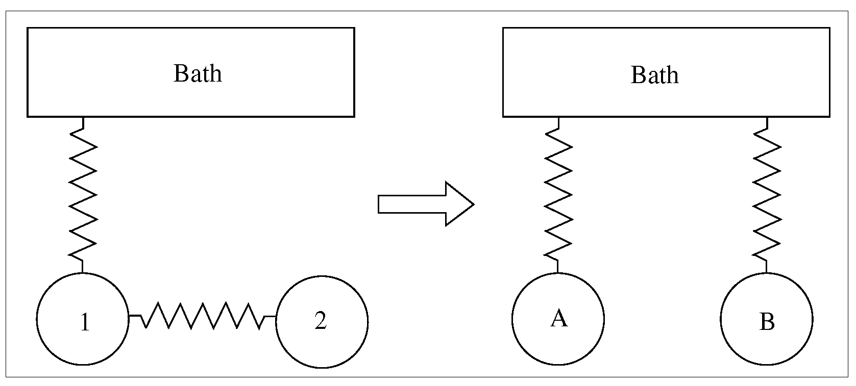
3. Performance of Coupled System

In this section, we study the effect of coupling in the performance of joint systems as the working media of Otto cycle. First, we consider two identical oscillators coupled via positions and momenta and then we consider spins coupled though Heisenberg XY model.

3.1. Coupled Oscillators

Consider two oscillators (labeled as 1 and 2) with same mass and frequency, and consider that they are coupled through their positions and momenta. The total Hamiltonian of the composite system reads [40,41,42]:

$$\begin{array}{cc}\hfill H^{\mathrm{os}}& =\frac{p_1^2}{2m}+\frac{p_2^2}{2m}+\frac{m{\mathsf{\Omega }}^2}{2}{x}_1^2+\frac{m{\mathsf{\Omega }}^2}{2}{x}_2^2\hfill \\ \hfill & +2\left(\frac{m\mathsf{\Omega }}{2}{\lambda }_x{x}_1{x}_2+\frac{1}{2m\mathsf{\Omega }}{\lambda }_p{p}_1{p}_2\right),\hfill \end{array}$$

(10)

where ${\lambda }_x$ and ${\lambda }_p$ are the coupling strengths with same units as that of $\mathsf{\Omega }$. We can write this Hamiltonian in terms of ladder operators ($c_i$ and $c_i^{†}$, where $i=1,2$) as,

$$\begin{array}{cc}\hfill H^{\mathrm{os}}& =\left(c_1^{†}{c}_1+c_2^{†}{c}_2+1\right)\mathsf{\Omega }+\frac{({\lambda }_x+{\lambda }_p)}{2}(c_1^{†}{c}_2+c_1{c}_2^{†})\hfill \\ \hfill & +\frac{({\lambda }_x-{\lambda }_p)}{2}(c_1{c}_2+c_1^{†}{c}_2^{†}).\hfill \end{array}$$

(11)

where $c_j^{†}=x_j\sqrt{m\mathsf{\Omega }/2}-i{p}_j/\sqrt{2m\mathsf{\Omega }}$ ($j=1,2$). For the quadratic coupling given in Equation (11), let us consider the following co-ordinate transformation,

$$\begin{array}{ccc}\hfill x_A=\frac{x_1+x_2}{\sqrt{2}},& & x_B=\frac{x_1-x_2}{\sqrt{2}};\hfill \end{array}$$

(12)

$$\begin{array}{ccc}\hfill p_A=\frac{p_1+p_2}{\sqrt{2}},& & p_B=\frac{p_1-p_2}{\sqrt{2}}.\hfill \end{array}$$

(13)

The Hamiltonian in terms of new coordinates reads,

$$\begin{array}{ccc}\hfill H^{\mathrm{os}}& =& \frac{p_A^2}{2M_A}+\frac{M_A{\mathsf{\Omega }}_A^2}{2}{x}_A^2+\frac{p_B^2}{2M_B}+\frac{M_B{\mathsf{\Omega }}_B^2}{2}{x}_B^2\hfill \end{array}$$

(14)

$$\begin{array}{cc}=& \left(c_A^{†}{c}_A+\frac{1}{2}\right){\mathsf{\Omega }}_A+\left(c_B^{†}{c}_B+\frac{1}{2}\right){\mathsf{\Omega }}_B,\hfill \end{array}$$

(15)

where $c_k^{†}$ and $c_k$, where $k=A,B$, are the creation and annihilation operators for the oscillators A and B. Here ${\mathsf{\Omega }}_A$ and ${\mathsf{\Omega }}_B$ are eigenmode frequencies and $M_A$ and $M_B$ are the effective masses in the new co-ordinate frame and the explicit expressions are given as,

$$\begin{array}{ccc}\hfill M_{A/B}& =& \frac{m\mathsf{\Omega }}{(\mathsf{\Omega }\pm {\lambda }_p)},\hfill \end{array}$$

(16)

$$\begin{array}{ccc}\hfill {\mathsf{\Omega }}_{A/B}& =& \sqrt{(\mathsf{\Omega }\pm {\lambda }_p)(\mathsf{\Omega }\pm {\lambda }_x)}.\hfill \end{array}$$

(17)

Note that, in the new frame, the modes (A and B) are uncoupled. Now consider the above mentioned Otto cycle in which $\mathsf{\Omega }$ is changed from its initial value $\omega$ to ${\omega }^{\prime }$ in the first adiabatic process. Correspondingly, the eigenfrequency for the oscillator A changes from ${\omega }_A$ to ${\omega }_A^{\prime }$ and similarly, frequency changes from ${\omega }_B$ to ${\omega }_B^{\prime }$ in the case of oscillator B. The eigenfrequencies return to the respective initial values in the second adiabatic process. Here one can consider that the working medium consists of two independent oscillators. Hence the total work done by the system can be considered as the sum of the contributions from independent oscillators. Note that ${\omega }_A$ and ${\omega }_B$ (${\omega }_A^{\prime }$ and ${\omega }_B^{\prime }$ ) are the effective frequencies of the subsystems after the co-ordinate transformation. Therefore they are functions of actual frequencies $\omega$ (${\omega }^{\prime }$) and coupling strengths. Hence ${\omega }_A$ and ${\omega }_B$ (${\omega }_A^{\prime }$ and ${\omega }_B^{\prime }$ ) are controlled by changing the frequencies of the actual subsystems. It can be done by changing potential in the case of oscillators or by changing the external magnetic field for the spins (see Section 3.2). We assume that there is no cross over of energy levels of the total Hamiltonian during the adiabatic process. The density matrix may change during the adiabatic process. However, the process is slow enough such that the populations at the instantaneous eigenstates of the Hamiltonian remain same (quantum adiabatic theorem). As discussed in Section 2.1, the total amount of heat absorbed by the system from hot reservoir is given by

$$\begin{array}{cc}\hfill Q& =\frac{{\omega }_A}{2}\left(\coth \left[\frac{{\beta }_h{\omega }_A}{2}\right]-coth\left[\frac{{\beta }_c{\omega }_A^{\prime }}{2}\right]\right)\hfill \\ \hfill & +\frac{{\omega }_B}{2}\left(\coth \left[\frac{{\beta }_h{\omega }_B}{2}\right]-coth\left[\frac{{\beta }_c{\omega }_B^{\prime }}{2}\right]\right).\hfill \end{array}$$

(18)

The first term denotes the heat absorbed by the system A ($Q_A$) and the second term represents the heat absorbed by the system B ($Q_B$). Similarly, the total work is the sum of the work done by the independent systems, $W=W_A+W_B$. Thus here

$$\begin{array}{cc}\hfill W& =\frac{({\omega }_A-{\omega }_A^{\prime })}{2}\left(\coth \left[\frac{{\beta }_h{\omega }_A}{2}\right]-coth\left[\frac{{\beta }_c{\omega }_A^{\prime }}{2}\right]\right)\hfill \\ \hfill & +\frac{({\omega }_B-{\omega }_B^{\prime })}{2}\left(\coth \left[\frac{{\beta }_h{\omega }_B}{2}\right]-coth\left[\frac{{\beta }_c{\omega }_B^{\prime }}{2}\right]\right).\hfill \end{array}$$

(19)

The efficiency of the individual system is given as ${\eta }_k=1-{\omega }_k^{\prime }/{\omega }_k$, where $k=\{A,B\}$. However, the actual efficiency of the coupled system is defined as the ratio of total work over the total heat absorbed by the system. So we can write

$$\eta =\frac{W_A+W_B}{Q_A+Q_B}=\frac{{\eta }_A{Q}_A+{\eta }_B{Q}_B}{Q_A+Q_B}.$$

(20)

When both the systems are working in engine mode (i.e., $Q_A>0$ and $Q_B>0$), we can write the above equation as

$$\eta ={\eta }_A\alpha +{\eta }_B(1-\alpha )$$

(21)

where $\alpha =Q_A/(Q_A+Q_B)\le 1$. Therefore we can write

$$\min \{{\eta }_A,{\eta }_B\}\le \eta \le \max \{{\eta }_A,{\eta }_B\}.$$

(22)

Therefore, when both independent oscillators work as an engine, the actual efficiency of the engine is bounded above and below by the efficiencies of the independent oscillators. For certain parameter values (see Section 4.1), one of the independent oscillators can work as refrigerator. In that case, the efficiency of the system is upper bounded by the efficiency of the other independent subsystem working as the engine.

Generalization

Now consider an Otto cycle, where the global parameter $\lambda$ (${\lambda }_x$ or ${\lambda }_p$ or both) is externally controlled and varied in the adiabatic branches, keeping $\mathsf{\Omega }$ fixed (see Figure 2). Even in this case, using the following analysis, one can show the existence of the non-trivial bounds for the efficiency. In this paper, we consider those quadratic couplings for which we can write the total Hamiltonian as the sum of the Hamiltonians of two independent subsystems under some co-ordinate transformation. Let us consider the Hamiltonian $H=H_A\oplus H_B$ at the end of Stage 1 and before the first adiabatic process (Stage 2) and $H^{\prime }=H_A^{\prime }\oplus H_B^{\prime }$ be the Hamiltonian at the end of the first adiabatic process. Before the starting of the adiabatic process, the system is in a thermal state and hence we can write the initial state as $\rho ={\rho }_A\otimes {\rho }_B$ in the eigenbasis of $H=H_A\oplus H_B$. Further, the adiabatic process ensures that the populations in the instantaneous eigenstates of the Hamiltonian remain unchanged during the process. Therefore, we can write the density matrix of the final state as ${\rho }^{\prime }={\rho }_A^{\prime }\otimes {\rho }_B^{\prime }$ in the basis of $H_A^{\prime }\oplus H_B^{\prime }$. For example, consider the coupled spin systems after the first thermalization process. Let us suppose $E_A^1$ and $E_A^2$ are the energy eigenvalues for the independent subsystem A with the corresponding populations $p_A^1$ and $p_A^2$ ($p_A^1+p_A^2=1$) respectively. Similarly, $E_B^1$ and $E_B^2$ are the energy eigenvalues for the second spin B with populations $p_B^1$ and $p_B^2$ ($p_B^1+p_B^2=1$) respectively. So the total energy can be written as

$$\begin{array}{c}\hfill \sum _{m=1}^2{p}_A^m{E}_A^m+\sum _{n=1}^2{p}_B^n{E}_B^n=\sum _{k=1}^2\sum _{l=1}^2(E_A^k+E_B^l)p_A^k{p}_B^l\end{array}$$

(23)

The terms $\left\{(E_A^k+E_B^l)\right\}$ and $\left\{p_A^k{p}_B^l\right\}$ in the right hand side represent the energy eigenvalues of the composite system and the corresponding populations respectively. At the end of the adiabatic process, the energy eigenvalues of the composite system changes but the Hamiltonian structure allows us to write it as the sum of the contributions from two independent subsystems. Therefore the energy eigenvalues at the end of the adiabatic process are given as $\left\{(E_A^{\prime k}+E_B^{\prime l})\right\}$. However, the corresponding populations remains fixed because of the quantum adiabatic theorem. Hence we can write

$$\begin{array}{c}\hfill \sum _{k=1}^2\sum _{l=1}^2(E_A^{\prime k}+E_B^{\prime l})p_A^k{p}_B^l=\sum _{m=1}^2{p}_A^m{E}_A^{\prime m}+\sum _{n=1}^2{p}_B^n{E}_B^{\prime n}\end{array}$$

(24)

Therefore the populations of the eigenstates of the independent subsystems are also unchanged during the process. Similar characteristics can be observed in the second adiabatic process also. Hence the total system can be considered as composition of two independent subsystems in the beginning as well as at the end of each process in the cycle. So, the total heat (or work) is the sum of the heat (or work) obtained from its independent subsystems. Therefore, the efficiency of the system will be bounded above and below by the efficiencies of the independent systems (Equation (22)).

An isothermal process can be simulated by an infinite number of infinitesimal adiabatic and isochoric processes [43]. As discussed above, in the adiabatic and isochoric processes, the work and the heat contributions from individual subsystems can be identified separately. Therefore, the isothermal process of the total system can be considered equivalent to the isothermal processes of two independent subsystems taken together. To understand the generality of the bounds of the efficiency observed in Otto cycle, we can consider other cycles such as Carnot cycle consisting of two isothermal processes and two adiabatic processes, and Stirling cycle consisting of two isothermal processes and two isochoric processes [35,39,44] (see Figure 3). Like the Otto cycle, in the Stirling cycle, the global efficiency is bounded by the efficiencies of independent subsystems because at any stage of the cycle, the total system can be decomposed into two independent subsystems. This shows that the analysis on the bounds of the efficiency represented in Equation (22) is a generic one and applicable to some of the other cycles also. Using similar analysis, we can also show that for a quantum Carnot cycle, both the independent subsystems work at Carnot efficiency, which is same as the global efficiency, i.e., $\eta ={\eta }_A={\eta }_B=1-T_c/T_h$.

3.2. Coupled Spin System

In order to compare the performance of the quantum Otto cycle with coupled oscillator and that with coupled spin-1/2 system, let us now consider two spin-1/2 systems coupled via Heisenberg exchange interaction, placed in a magnetic field applied along the z-direction. The Hamiltonian in terms of spin operators are given by

$$H^{\mathrm{sp}}=\mathsf{\Omega }(S_1^z\otimes I+I\otimes S_2^z)+2(J_x{S}_1^x{S}_2^x+J_y{S}_1^y{S}_2^y),$$

(25)

where $J_x$ and $J_y$ are the interaction constants along x and y directions. This model is generally known as Heisenberg XY model. Adding an equal energy with each level, we can write the Hamiltonian in terms of raising and lowering operators ($S_i^{+}$ and $S_i^{-}$, where $i=1,2$) as

$$\begin{array}{cc}\hfill H^{\mathrm{sp}}=& (S_1^{+}{S}_1^{-}+S_2^{+}{S}_2^{-}+1)\mathsf{\Omega }\hfill \\ \hfill & +\frac{(J_x+J_y)}{2}(S_1^{+}{S}_2^{-}+S_1^{-}{S}_2^{+})\hfill \\ \hfill & +\frac{(J_x-J_y)}{2}(S_1^{+}{S}_2^{+}+S_1^{-}{S}_2^{-}).\hfill \end{array}$$

(26)

Equations (11) and (26) have the similar form. As we have seen in the case of oscillators, Equation (26) can be written as the sum of the Hamiltonians of independent subsystems. Therefore, the efficiency of the system is bounded from above and below by the efficiencies of independent subsystems as given in Equation (22). In the following section (Section 4), we compare the performances of coupled spins and coupled oscillators when they undergo separately the quantum Otto cycles for different values of ${\lambda }_x$, ${\lambda }_p$, $J_x$, and $J_y$.

3.3. Optimal Work

As we have seen in Equations (4) and (8), work is a function of $\omega$ and ${\omega }^{\prime }$. The optimal work can be estimated by maximizing work with respect to $\omega$ and ${\omega }^{\prime }$. Now suppose that work is maximum at $\omega ={\omega }^{*}$ and ${\omega }^{\prime }={\omega }^{\prime *}$. Therefore, for two uncoupled oscillators, maximum work occurs when both the system work with ${\omega }^{*}$ and ${\omega }^{\prime *}$. Now consider ${\mathsf{\Omega }}_A$ and ${\mathsf{\Omega }}_B$ are frequencies of the independent modes A and B of the coupled oscillators respectively, before the first adiabatic process and ${\mathsf{\Omega }}_A^{\prime }$ and ${\mathsf{\Omega }}_B^{\prime }$ are the frequencies of the independent modes A and B respectively, after the first adiabatic process. Then, ${\mathsf{\Omega }}_A$ and ${\mathsf{\Omega }}_B$ (${\mathsf{\Omega }}_A^{\prime }$ and ${\mathsf{\Omega }}_B^{\prime }$) are functions of $\omega$, ${\lambda }_x$ and ${\lambda }_p$ (${\omega }^{\prime }$, ${\lambda }_x$ and ${\lambda }_p$). Similar arguments can be made for coupled spins too. Therefore, if the subsystem A provides optimal work, then the work obtained from the subsystem B may not be optimal because ${\mathsf{\Omega }}_A$ and ${\mathsf{\Omega }}_B$ (${\mathsf{\Omega }}_A^{\prime }$ and ${\mathsf{\Omega }}_B^{\prime }$) are not independent. Therefore we have

$$W_{\lambda }^{\max }\le W_0^{\max },$$

(27)

$W_{\lambda }^{\max }$ and $W_0^{\max },$ are the maximum values of work obtained from the coupled and uncoupled systems respectively. The equality holds for the case where both independent subsystems have the same frequency.

Generalization

Now consider a cycle in which the global parameters ${\lambda }_x$ and ${\lambda }_p$ or $J_x$ and $J_y$ are varied in the adiabatic branches instead of varying $\mathsf{\Omega }$. Because of quadratic coupling, we can show that the total system consists of two independent subsystems, throughout the cycle. Then the total work is the sum of the contributions from its independent subsystems and therefore Equation (27) holds even when we change global parameters to extract work.

In Stirling cycle and in Carnot cycle, for a working medium with quadratic interaction, we can always write the total work as the sum of the contributions from its independent subsystems. Therefore, using the argument mentioned above, we can say that Equation (27) holds in general.

In Section 4 and Section 5, we discuss the Otto cycle in detail by considering certain special cases.

4. Special Cases

In this section, we discuss the performance of the Otto cycle when the coupled systems with specific values of interaction constants constitute as the working medium. In Section 4.1, we take $J_x=J_y$ in the case of spin, which is known as Heisenberg XX model. Analogous interaction in oscillators is achieved by setting ${\lambda }_x={\lambda }_p$. Another interesting model is obtained with values $J_x=-J_y$ in spins and ${\lambda }_x=-{\lambda }_p$ in oscillators, are discussed in Section 4.3.

4.1. XX Model

Let us consider the following case: ${\lambda }_x=J_x={\lambda }_p=J_y={\lambda }_J\left(\mathrm{say}\right)$. For coupled oscillators, we can write the Hamiltonian in Equation (11) in terms of ladder operators as

$$\begin{array}{c}\hfill H^{\mathrm{os}}=\left(c_1^{†}{c}_1+c_2^{†}{c}_2+1\right)\mathsf{\Omega }+{\lambda }_J(c_1^{†}{c}_2+c_1{c}_2^{†}).\end{array}$$

(28)

From Equation (16), we get the frequencies of the independent modes as ${\mathsf{\Omega }}_A=\mathsf{\Omega }+{\lambda }_J$ and ${\mathsf{\Omega }}_B=\mathsf{\Omega }-{\lambda }_J$. Therefore, inside the Otto cycle where the value of $\mathsf{\Omega }$ is varied from $\omega$ to ${\omega }^{\prime }$ during the first adiabatic process, we have ${\omega }_{A/B}=\omega \pm {\lambda }_J$ and ${\omega }_{A/B}^{\prime }={\omega }^{\prime }\pm {\lambda }_J$. In the new co-ordinates, the oscillators are independent. Hence the total heat absorbed from the hot reservoir is the sum of the heat absorbed by the independent subsystems A and B. Substituting the values of ${\omega }_A$, ${\omega }_A^{\prime }$, ${\omega }_B$ and ${\omega }_B^{\prime }$ in Equations (18) and (19), we get the expressions for the heat and the work respectively. The explicit expression for the work obtained from Equation (19) is given as

$$\begin{array}{cc}\hfill W^{\mathrm{os}}& =C\left(\coth \left[\frac{(\omega -{\lambda }_J)}{2T_h}\right]-coth\left[\frac{({\omega }^{\prime }-{\lambda }_J)}{2T_c}\right]\right)\hfill \\ \hfill & +C\left(\coth \left[\frac{(\omega +{\lambda }_J)}{2T_h}\right]-coth\left[\frac{({\omega }^{\prime }+{\lambda }_J)}{2T_c}\right]\right),\hfill \end{array}$$

(29)

where $C=(\omega -{\omega }^{\prime })/2$. The efficiency of the independent subsystems are obtained as

$${\eta }_A=\frac{(\omega -{\omega }^{\prime })}{(\omega +{\lambda }_J)}\mathrm{and}{\eta }_B=\frac{(\omega -{\omega }^{\prime })}{(\omega -{\lambda }_J)}.$$

(30)

So we have ${\eta }_B>{\eta }_A$. Interestingly, the upper bound ${\eta }_B$ is analogous to the upper bound of the efficiency obtained for the coupled spins with isotropic Heisenberg Hamiltonian [27]. Now we calculate the global efficiency as the ratio of the total work ($W_A+W_B$) by the total heat ($Q_A+Q_B$). We get the global efficiency by substituting the values of ${\omega }_A$, ${\omega }_A^{\prime }$, ${\omega }_B$ and ${\omega }_B^{\prime }$ in Equation (20). Now we expand this efficiency for small coupling constant ${\lambda }_J$ up to the third order, and we get:

$$\begin{array}{cc}\hfill {\eta }^{\mathrm{os}}=1-\frac{{\omega }^{\prime }}{\omega }& +\frac{\gamma \left(T_c{\mathrm{csch}}^2\left[\frac{\omega }{2T_h}\right]-T_h{\mathrm{csch}}^2\left[\frac{{\omega }^{\prime }}{2T_c}\right]\right){\lambda }_J^2}{2\left(coth\left[\frac{\omega }{2T_h}\right]-coth\left[\frac{{\omega }^{\prime }}{2T_c}\right]\right)}\hfill \\ \hfill & +O\left[{\lambda }_J^4\right],\hfill \end{array}$$

(31)

where $\gamma =(\omega -{\omega }^{\prime })/\left(T_h{T}_c{\omega }^2\right)$ and $\mathrm{csch}\left(x\right)\equiv \mathrm{cosech}\left(x\right)$.

We need to compare the performance of the oscillator system with that of the coupled spin system as a heat engine. For that, we consider two spin-1/2 systems coupled via Heisenberg XX Hamiltonian ($J_x=J_y$). Representing this Hamiltonian in terms of ladder operators, it takes similar form of the Hamiltonian that we considered in the case of oscillators (see below). Therefore we write,

$$H^{\mathrm{sp}}=(S_1^{+}{S}_1^{-}+S_2^{+}{S}_2^{-}+1)\mathsf{\Omega }+{\lambda }_J(S_1^{+}{S}_2^{-}+S_1^{-}{S}_2^{+}).$$

(32)

Coefficient $\mathsf{\Omega }$ of $\left(c_1^{†}{c}_1+c_2^{†}{c}_2+1\right)$ in Equation (28) is characteristically same as the coefficient $\mathsf{\Omega }$ of $(S_1^{+}{S}_1^{-}+S_2^{+}{S}_2^{-}+1)$ in Equation (32). Same is true with the coefficient ${\lambda }_J$ appeared in Equations (28) and (32). To compare the performance of coupled spins and oscillators, we can diagonalize the Hamiltonian for the coupled spins so that in the new basis, spins are uncoupled. So we can write

$$H^{\mathrm{sp}}=(\mathsf{\Omega }+{\lambda }_J)(S_A^{+}{S}_A^{-}+\frac{1}{2})+(\mathsf{\Omega }-{\lambda }_J)(S_B^{+}{S}_B^{-}+\frac{1}{2}).$$

(33)

Therefore, the total heat exchanged between the system and the hot bath is the sum of contributions from spins A and B. So we get the heat exchanged between system k (A or B) and the hot bath as (see Equation (7))

$$Q_k^{\mathrm{sp}}=\frac{{\omega }_k}{2}\left(\tanh \left[\frac{{\omega }_k^{\prime }}{2T_c}\right]-tanh\left[\frac{{\omega }_k}{2T_h}\right]\right).$$

(34)

The total heat exchange between the system and the hot bath is $Q^{\mathrm{sp}}=Q_A^{\mathrm{sp}}+Q_B^{\mathrm{sp}}$ The total work done by the system is the sum of the contributions from the individual spins defined in the new basis. So we get

$$\begin{array}{cc}\hfill W^{\mathrm{sp}}& ={\eta }_A{Q}_A^{\mathrm{sp}}+{\eta }_B{Q}_B^{\mathrm{sp}}\hfill \\ \hfill W^{\mathrm{sp}}& =C\left(\tanh \left[\frac{({\omega }^{\prime }-{\lambda }_J)}{2T_c}\right]-tanh\left[\frac{(\omega -{\lambda }_J)}{2T_h}\right]\right)\hfill \\ \hfill & +C\left(\tanh \left[\frac{({\omega }^{\prime }+{\lambda }_J)}{2T_c}\right]-tanh\left[\frac{(\omega +{\lambda }_J)}{2T_h}\right]\right),\hfill \end{array}$$

(35)

with $C=(\omega -{\omega }^{\prime })/2$. Here, ${\eta }_A$ and ${\eta }_B$ are same as that obtained in coupled oscillators given in Equation (30). Therefore, the efficiency of the engine is given as

$${\eta }^{\mathrm{sp}}=\frac{{\eta }_A{Q}_A^{\mathrm{sp}}+{\eta }_B{Q}_B^{\mathrm{sp}}}{Q_A^{\mathrm{sp}}+Q_B^{\mathrm{sp}}}.$$

(36)

We can expand this efficiency for small values of ${\lambda }_J$ as

$$\begin{array}{cc}\hfill {\eta }^{\mathrm{sp}}=1-\frac{{\omega }^{\prime }}{\omega }& +\frac{\gamma \left(T_h{\mathrm{sech}}^2\left[\frac{{\omega }^{\prime }}{2T_c}\right]-T_c{\mathrm{sech}}^2\left[\frac{\omega }{2T_h}\right]\right){\lambda }_J^2}{2\left(tanh\left[\frac{\omega }{2T_h}\right]-tanh\left[\frac{{\omega }^{\prime }}{2T_c}\right]\right)}\hfill \\ \hfill & +O\left[{\lambda }_J^4\right].\hfill \end{array}$$

(37)

The difference in the efficiencies obtained from coupled oscillators and coupled spins for small coupling is calculated from Equations (31) and (37). When the coupling ${\lambda }_J=0$, both oscillator as well as spin system yields the same efficiency as discussed in Section 2. By introducing a small coupling between the systems, we can write the difference between the efficiencies of the oscillator model and the spin model as

$$\begin{array}{cc}\hfill {\eta }^{\mathrm{os}}-{\eta }^{\mathrm{sp}}& =\gamma \left(T_c\mathrm{csch}\left[\frac{\omega }{T_h}\right]+T_h\mathrm{csch}\left[\frac{{\omega }^{\prime }}{T_c}\right]\right){\lambda }_J^2\hfill \\ \hfill & >0,\hfill \end{array}$$

(38)

since $\omega >{\omega }^{\prime }$ and $\gamma >0$. Hence in this model, for small values of ${\lambda }_J$, the efficiency achieved by coupled oscillators is higher than the efficiency obtained from coupled spin model. Now we can see the behavior of the efficiency as a function of ${\lambda }_J$ (see Figure 4). The characteristics of the efficiencies in Figure 4 remain the same with the choice of different values of $T_h$, $T_c$, $\omega$, and ${\omega }^{\prime }$. When ${\omega }_A^{\prime }/T_c\ge {\omega }_A/T_h$ (${\omega }_A^{\prime }<{\omega }_A$) and ${\omega }_B^{\prime }/T_c\ge {\omega }_B/T_h$ (${\omega }_B^{\prime }<{\omega }_B$), both the independent systems work as engines. It is interesting to note that when ${\lambda }_J=({\omega }^{\prime }{T}_h-\omega T_c)/(T_h-T_c)={\lambda }_c\left(\mathrm{say}\right)$, the upper bound of the efficiency, which is the efficiency of oscillator B, attains the Carnot value (${\omega }_B^{\prime }/T_c={\omega }_B/T_h$) with zero work output. At this point, the global efficiency of the system is equal to the efficiency of oscillator A, ${\eta }^{\mathrm{os}}={\eta }^{\mathrm{sp}}={\eta }_A$. When ${\lambda }_J>{\lambda }_c$, oscillator B works as refrigerator, which in turn reduces the efficiency of the engine. Hence the efficiency of the total system lies below the efficiency of oscillator A. Now we can compare the performance in terms of work given in Equations (29) and (35). The terms on the right-hand side of these equations are positive when both the independent systems work in the engine mode. In that case, using the analysis made in Section 2 for uncoupled systems, we can show that $W^{\mathrm{os}}>W^{\mathrm{sp}}$.

4.2. Optimal Work and Correlations

In the thermodynamic cycle, the origin of any correlation between the actual subsystems is due to the coupling. When the system thermalizes at the end of stage 1 and stage 3, the state of the system becomes a product state irrespective of the initial state, if there is no coupling present in the system. The proof that the optimum work extractable from a coupled system is upper bounded by the optimum work obtained from the uncoupled system (Equation (27)) implies that the presence of quantum correlations do not have any advantage in optimal work extraction. To illustrate this fact (see also Section 3.3) with an example, we analyze the behavior of work versus concurrence for the coupled spin systems. The concurrence is a measure of entanglement of an arbitrary two qubit state [45,46,47]. The concurrence has one to one correspondence with the entanglement of formation. The concurrence of a state $\rho$ is defined as

$$C=\mathrm{Max}\{0,\sqrt{{\lambda }_1}-\sqrt{{\lambda }_2}-\sqrt{{\lambda }_3}-\sqrt{{\lambda }_4}\}$$

(39)

where ${\lambda }_1$, ${\lambda }_2$, ${\lambda }_3$ and ${\lambda }_4$ are the eigenvalues of the matrix R written in descending order. The Matrix R is defined as $R=\rho ({\sigma }_y\otimes {\sigma }_y){\rho }^{*}({\sigma }_y\otimes {\sigma }_y)$ where ${\sigma }_y$ is the Pauli matrix. We estimate the concurrences for the thermal states at the end of Stage 1 and Stage 3 denoted as $C_h$ and $C_c$ respectively [26]. For the numerical analysis shown in Figure 5, we fix the temperatures of the hot and the cold bath, then we randomly choose the values of $\omega$, ${\omega }^{\prime }$ and ${\lambda }_J=J_x=J_y$ such that system should work as an engine. The optimum work is obtained only for zero concurrence and hence the numerical analysis shows that our theoretically obtained bound for the work holds.

In Figure 5, the work decreases and then increases with the concurrence. This is due to the fact that, for the coupled systems, the engine can work in two regimes, $\omega >{\omega }^{\prime }$ as well as ${\omega }^{\prime }>\omega$ as discussed in [27]. The maximum work at given values of $C_h$ and $C_c$ is another interesting direction to study.

4.3. XY Model

Here we consider the case ${\lambda }_x=J_x=-{\lambda }_p=-J_y={\lambda }_J$ (say). The Hamiltonian corresponding to the coupled oscillators is now written as

$$H^{\mathrm{os}}=\left(c_1^{†}{c}_1+c_2^{†}{c}_2+1\right)\mathsf{\Omega }+{\lambda }_J(c_1^{†}{c}_2^{†}+c_1{c}_2).$$

(40)

In the new co-ordinate system (described by Equation (17)), both the independent oscillators have the same frequency, which is given by ${\mathsf{\Omega }}_A={\mathsf{\Omega }}_B=\sqrt{({\mathsf{\Omega }}^2-{\lambda }_J^2)}$. Therefore, in the cycle, we have ${\omega }_A={\omega }_B=\sqrt{({\omega }^2-{\lambda }_J^2)}$ and ${\omega }_A^{\prime }={\omega }_B^{\prime }=\sqrt{({\omega }^{\prime 2}-{\lambda }_J^2)}$. Hence, we get ${\eta }_A={\eta }_B=1-{\omega }_A^{\prime }/{\omega }_A$ and from Equation (21), we obtain

$${\eta }^{\mathrm{os}}={\eta }_A=1-\sqrt{\frac{{\omega }^{\prime 2}-{\lambda }_J^2}{{\omega }^2-{\lambda }_J^2}}.$$

(41)

On the other hand, in the spin case, the analogous Hamiltonian is an example of Heisenberg XY model. In this case, the interaction Hamiltonian has the following form $H_{int}=J(S_1^x{S}_2^x-S_1^y{S}_2^y)$, where J is the interaction constant. This model is well studied as quantum Otto cycle [24,25]. In terms of raising and lowering operators, we can write the spin Hamiltonian as

$$\begin{array}{cc}\hfill H^{\mathrm{sp}}& =(S_1^{+}{S}_1^{-}+S_2^{+}{S}_2^{-}+1)\mathsf{\Omega }+{\lambda }_J(S_1^{+}{S}_2^{+}+S_1^{-}{S}_2^{-})\hfill \\ \hfill & ={\mathsf{\Omega }}_A(S_A^{+}{S}_A^{-}+\frac{1}{2})+{\mathsf{\Omega }}_B(S_B^{+}{S}_B^{-}+\frac{1}{2}),\hfill \end{array}$$

(42)

where ${\mathsf{\Omega }}_A={\mathsf{\Omega }}_B=\sqrt{{\mathsf{\Omega }}^2+{\lambda }_J^2}$. Therefore, we have two independent spins with the same frequency. So one would expect the efficiency of this system is similar to that of a single system (or two uncoupled systems) given in Equation (9). This is true only when Stage 2 and Stage 4 are done slow enough. Because, in this case, the eigenvectors of the Hamiltonian are functions of $\mathsf{\Omega }$ and ${\lambda }_J$. Hence, when the system works as Otto cycle, by changing the magnetic field associated with the system, internal friction appears to be depending upon the rate at which magnetic field is changed [24,25]. This is due to the non-commutativity of the Hamiltonian at different instances during the driving. Here the adiabatic processes are done slow enough so that quantum adiabatic theorem holds. Since the energy level spacings for both the independent subsystems are equal (${\mathsf{\Omega }}_A={\mathsf{\Omega }}_B$) in Equation (42), these subsystems undergo identical cycles with the same efficiency. Therefore, the global efficiency is also equal to the efficiency of the subsystem, which is given by

$${\eta }^{\mathrm{sp}}=1-\sqrt{\frac{{\omega }^{\prime 2}+{\lambda }_J^2}{{\omega }^2+{\lambda }_J^2}}.$$

(43)

Now comparing Equations (41) and (43), we get ${\eta }^{\mathrm{os}}\ge {\eta }^{\mathrm{sp}}$, for a range of parameter such that the systems work as engines (where $|{\lambda }_J|$ may be also large). For a small coupling, we can expand the efficiencies of the coupled oscillators and coupled spin systems as

$${\eta }_{\mathrm{os}}=1-\frac{{\omega }^{\prime }}{\omega }+\frac{({\omega }^2-{\omega }^{\prime 2}){\lambda }_J^2}{2{\omega }^3{\omega }^{\prime }}+O\left[{\lambda }_J^4\right]$$

(44)

$${\eta }_{\mathrm{sp}}=1-\frac{{\omega }^{\prime }}{\omega }-\frac{({\omega }^2-{\omega }^{\prime 2}){\lambda }_J^2}{2{\omega }^3{\omega }^{\prime }}+O\left[{\lambda }_J^4\right]$$

(45)

Equation (44) shows that when the coupling is introduced, the efficiency of the coupled oscillators goes above the efficiency of the uncoupled model ${\eta }_{\mathrm{uc}}=1-{\omega }^{\prime }/\omega$ (Equations (5) and (9)), while, according to Equation (45), the efficiency of the spin system lies below that of the uncoupled model ${\eta }_{\mathrm{os}}>{\eta }_{\mathrm{uc}}>{\eta }_{\mathrm{sp}}$ (see Figure 7). Interestingly, Equations (44) and (45) shows the symmetric behavior of ${\eta }_{\mathrm{os}}$ and ${\eta }_{\mathrm{sp}}$ about ${\eta }_{\mathrm{uc}}$. This behavior is obvious due to the fact that coupling reduces the frequencies of the eigenmodes of the harmonic oscillators while it increases the energy level spacings of the independent spin systems.

5. Performance as a Refrigerator

The coupled spins and coupled oscillators can also work as a refrigerator [48,49]. In this section, we consider the case where both the independent subsystems (of coupled oscillators and coupled spins separately) work as refrigerators. The refrigeration cycle is same as the cycle described for engine in Section 2, provided refrigerators absorb heat from the cold bath ($Q_c>0$) and transfer it into the hot bath ($Q_h<0$). To transfer heat from the cold bath to the hot bath, work has to be done on the system and hence, we have $W=Q_h+Q_c<0$. The coefficient of performance (COP) is defined as $\zeta =Q_c/\left|W\right|$ [50,51].

If we consider a single spin or a single oscillator (See Section 2) such that the conditions on the parameters during the cycle are: $\omega >{\omega }^{\prime }$ and $\omega /T_h>{\omega }^{\prime }/T_c$, then these systems (spin or oscillator) work as refrigerators. So we get the COP as

$${\zeta }^{\mathrm{os}}={\zeta }^{\mathrm{sp}}=\frac{Q_c^{\mathrm{os}\left(\mathrm{sp}\right)}}{|W^{\mathrm{os}\left(\mathrm{sp}\right)}|}=\frac{{\omega }^{\prime }}{\omega -{\omega }^{\prime }}.$$

(46)

Therefore, for uncoupled oscillators and spins, COPs are equal. Now, consider the COP for coupled systems as described in Section 3. Suppose ${\omega }_A$ and ${\omega }_B$ are the frequencies of the subsystems (of coupled oscillators or coupled spins) A and B respectively, before the first adiabatic process and ${\omega }_A^{\prime }$ and ${\omega }_B^{\prime }$ are the frequencies of A and B at the end of the first adiabatic process. Then both the independent subsystems work as refrigerator when ${\omega }_A/T_h>{\omega }_A^{\prime }/T_c$ and ${\omega }_B/T_h>{\omega }_B^{\prime }/T_c$ with the conditions ${\omega }_A>{\omega }_A^{\prime }$ and ${\omega }_B>{\omega }_B^{\prime }$. Therefore, the local COP is ${\zeta }_k={\omega }_k^{\prime }/({\omega }_k-{\omega }_k^{\prime })$, where $k=A,B$. Further, the global COP is written as

$$\begin{array}{cc}\hfill \zeta & =\frac{{\zeta }_A|W_A|+{\zeta }_B\left|W_B\right|}{|W_A+W_B|}\hfill \\ \hfill & ={\alpha }^{\prime }{\zeta }_A+(1-{\alpha }^{\prime }){\zeta }_B,\hfill \end{array}$$

where ${\alpha }^{\prime }=|W_A|/(|W_A+W_B\left|\right)<1$. Since $W_A<0$ and $W_B<0$, we have $|W_A|+|W_B|=|W_A+W_B|$. Hence we can write

$$\min \{{\zeta }_A,{\zeta }_B\}\le \zeta \le \max \{{\zeta }_A,{\zeta }_B\}.$$

(47)

The global COP is bounded by COPs of the subsystems when both the subsystems work as refrigerators. Now our task is to understand the behavior of COPs for special cases as we have done for heat engine in Section 4.

5.1. XX Model

Here we compare the COPs of coupled oscillators and coupled spins when the coupling in each case is of $XX$ type. The COPs of subsystems are obtained as ${\zeta }_A=({\omega }^{\prime }+{\lambda }_J)/(\omega -{\omega }^{\prime })$ and ${\zeta }_B=({\omega }^{\prime }-{\lambda }_J)/(\omega -{\omega }^{\prime })$ and hence we have ${\zeta }_A>{\zeta }_B$. We calculate the global COP as ${\zeta }^{\mathrm{os}}=Q_c^{\mathrm{os}}/\left|W^{\mathrm{os}}\right|$. Expanding for small values of ${\lambda }_J$, we get

$$\begin{array}{cc}\hfill {\zeta }^{\mathrm{os}}& =\frac{{\omega }^{\prime }}{(\omega -{\omega }^{\prime })}+\frac{\left(T_h{\mathrm{csch}}^2\left[\frac{{\omega }^{\prime }}{2T_c}\right]-T_c{\mathrm{csch}}^2\left[\frac{\omega }{2T_h}\right]\right){\lambda }_J^2}{2{\gamma }^{\prime }\left(coth\left[\frac{\omega }{2T_h}\right]-coth\left[\frac{{\omega }^{\prime }}{2T_c}\right]\right)}\hfill \\ \hfill & +O\left[{\lambda }_J^4\right],\hfill \end{array}$$

(48)

where ${\gamma }^{\prime }=T_h{T}_c(\omega -{\omega }^{\prime })$. Similarly, for the spin systems, the COP is ${\zeta }^{\mathrm{sp}}=Q_c^{\mathrm{sp}}/\left|W^{\mathrm{sp}}\right|$. Further, expanding ${\zeta }^{\mathrm{sp}}$, we get

$$\begin{array}{cc}\hfill {\zeta }^{\mathrm{sp}}=\frac{{\omega }^{\prime }}{(\omega -{\omega }^{\prime })}& +\frac{\left(T_c{\mathrm{sech}}^2\left[\frac{\omega }{2T_h}\right]-T_h{\mathrm{sech}}^2\left[\frac{{\omega }^{\prime }}{2T_c}\right]\right){\lambda }_J^2}{2{\gamma }^{\prime }\left(tanh\left[\frac{\omega }{2T_h}\right]-tanh\left[\frac{{\omega }^{\prime }}{2T_c}\right]\right)}\hfill \\ \hfill & +O\left[{\lambda }_J^4\right]\hfill \end{array}$$

(49)

In each of the above two Equations (48) and (49), the first term on the right-hand side represents the COP of the uncoupled system. To compare the effects of coupling in COPs, we calculate the difference between ${\zeta }^{\mathrm{sp}}$ and ${\zeta }^{\mathrm{os}}$, which is given by

$$\begin{array}{c}\hfill {\zeta }^{\mathrm{sp}}-{\zeta }^{\mathrm{os}}=\frac{\left(T_c\mathrm{csch}\left[\frac{\omega }{T_h}\right]+T_h\mathrm{csch}\left[\frac{{\omega }^{\prime }}{T_c}\right]\right){\lambda }_J^2}{{\gamma }^{\prime }}>0\\ \hfill \end{array}$$

(50)

This means that a small coupling (${\lambda }_J$) introduced between the subsystems makes the coupled spins more efficient than the coupled oscillators in transferring heat from cold bath to hot bath, whereas a reverse effect is observed in the case of the heat engine (${\eta }^{\mathrm{sp}}<{\eta }^{\mathrm{os}}$) for small values of ${\lambda }_J$. An example is given in Figure 6. When both the subsystems work as refrigerators, the global COP is bounded by the COPs of the independent systems. When ${\lambda }_J=(\omega T_c-{\omega }^{\prime }{T}_h)/(T_h-T_c)={\lambda }_c^{\prime }$ (say), the refrigerator A attains Carnot value with no heat transfer from the cold reservoir to the hot reservoir. Therefore, the global COP reaches its lower bound. Further, for ${\lambda }_J>{\lambda }_c^{\prime }$, the system A does not work as a refrigerator and hence global COP is bounded from above by ${\zeta }_B$.

5.2. XY Model

Now we consider the COPs in the case of XY model as described in Section 4.3. In this model, for coupled oscillators, we have ${\omega }_A={\omega }_B=\sqrt{{\omega }^2-{\lambda }_J^2}$ and ${\omega }_A^{\prime }={\omega }_B^{\prime }=\sqrt{{\omega }^{\prime 2}-{\lambda }_J^2}$. Since both the independent oscillators are identical and having equal frequencies at various stages of the cycle, the COPs of the subsystems are equal to the global COP, which is given by

$$\begin{array}{ccc}\hfill {\zeta }^{\mathrm{os}}& =& \frac{1}{\sqrt{\frac{{\omega }^2-{\lambda }_J^2}{{\omega }^{\prime 2}-{\lambda }_J^2}}-1}.\hfill \end{array}$$

(51)

Similarly, in the case of coupled spins, we have ${\omega }_A={\omega }_B=\sqrt{{\omega }^2+{\lambda }_J^2}$ and ${\omega }_A^{\prime }={\omega }_B^{\prime }=\sqrt{{\omega }^{\prime 2}+{\lambda }_J^2}$. Both the independent subsystems have same energy level spacings and hence the subsystems work as refrigerators when ${\omega }_A/T_h>{\omega }_A^{\prime }/T_c$. Therefore the COPs of the subsystems are equal to the global COP, given by

$$\begin{array}{ccc}\hfill {\zeta }^{\mathrm{sp}}& =& \frac{1}{\sqrt{\frac{{\omega }^2+{\lambda }_J^2}{{\omega }^{\prime 2}+{\lambda }_J^2}}-1}.\hfill \end{array}$$

(52)

Therefore, we have ${\zeta }^{\mathrm{sp}}>{\zeta }^{\mathrm{os}}$ even for larger values of ${\lambda }_J$. On the contrary, from Equations (41) and (43), we have ${\eta }^{\mathrm{sp}}<{\eta }^{\mathrm{os}}$ for the engine. Now we can expand the COPs of the coupled systems for small values of ${\lambda }_J$.

$${\zeta }_{\mathrm{os}}=\frac{{\omega }^{\prime }}{(\omega -{\omega }^{\prime })}-\frac{(\omega +{\omega }^{\prime }){\lambda }_J^2}{2\omega {\omega }^{\prime }(\omega -{\omega }^{\prime })}+O\left[{\lambda }_J^4\right],$$

(53)

$${\zeta }_{\mathrm{sp}}=\frac{{\omega }^{\prime }}{(\omega -{\omega }^{\prime })}+\frac{(\omega +{\omega }^{\prime }){\lambda }_J^2}{2\omega {\omega }^{\prime }(\omega -{\omega }^{\prime })}+O\left[{\lambda }_J^4\right].$$

(54)

Since $\omega >{\omega }^{\prime }$, by introducing the coupling, the COP of the coupled spins becomes higher than that of of the uncoupled spins, ${\zeta }_{\mathrm{uc}}={\omega }^{\prime }/(\omega -{\omega }^{\prime })$ (Equaton (46)), while the COP of oscillators lies below ${\zeta }_{\mathrm{uc}}$. It is interesting to note that exactly the opposite behavior is observed in the case of heat engine (see Equations (44) and (45)) . This behaviour is shown in Figure 7.

6. Discussion and Future Direction

To conclude, we analyzed the performances of coupled oscillators and coupled spins as heat engines and refrigerators. In both the cases, we choose suitable co-ordinate transformation to get two independent subsystems. The global figure of merit is bounded by the figures of merit of the independent subsystems. When the upper bound is Carnot value, the global figure of merit reaches the lower bound. For the case of the heat engine, when one of the subsystems works as a refrigerator, the global efficiency falls below the lower bound. Similarly, for the case of the refrigerator, the global COP falls below the lower bound when one of the subsystems work as a heat engine. The upper bound is tighter than the Carnot bound. For the systems considered in this work, it is also shown that the optimal work extractable from the coupled system is upper bounded by the optimal work extractable from the uncoupled system. Whether this is a generic feature for arbitrary coupled systems with quadratic coupling is a question of future interest. However, the figures of merit such as efficiency or COP can have higher values in the presence of coupling. We point out the range of parameters and some forms of interactions where the efficiency of the coupled oscillators is higher than that of the coupled spins, whereas the global COP is higher for coupled spins compared to coupled oscillators. Therefore, coupling causes opposite effects in the figures of merit of heat engine and refrigerator.

An interesting query is as to whether the entanglement between the coupled systems is responsible for the gap in the efficiencies, i.e., the difference between the efficiencies obtained from coupled oscillators and coupled spins. Our preliminary observation shows that the entanglement does not have any role in creating this gap. On the other hand, we have shown that the quantum correlations do not help in extracting optimal work. A recent study in optomechanical heat engine shows the reduction in extractable work due to quantum correlations [52].

One may try to look at the efficiency ${\eta }_1^{\mathrm{sp}}$ of coupled system of two spin-1 particles to look for a possible ordering of the form ${\eta }_{1/2}^{\mathrm{sp}}\le {\eta }_1^{\mathrm{sp}}\le {\eta }^{\mathrm{os}}$, where ${\eta }_{1/2}^{\mathrm{sp}}$ is efficiency in the case of a coupled spin-1/2 particles. In the case of coupled qutrits with $XX$ coupling, the independent spins do not have energy level spacings $\omega \pm {\lambda }_J$ unlike in the case of coupled spin-1/2 systems and coupled oscillators as discussed in Section 4.1 [53]. So the efficiency of the coupled qutrits may not exactly fall in between the efficiency curves obtained for coupled spin-1/2 systems and coupled oscillators. Therefore, an interesting future direction is to investigate the form of interaction for which a monotonic behavior of the efficiency with the increment in the dimension of the system is exhibited.

As mentioned in Section 2, the adiabatic processes should be done slow enough to avoid creation of coherence between the eigenstates of the Hamiltonian. These coherences create a frictional effect in the system, which in turn reduces the extractable work. The second assumption is that the system is attached to the respective baths for long enough time till the system attains equilibrium. Thermalization of coupled oscillators can be modeled with coupled micro-cavities as described in Reference [41]. In this model, one of the system (say system 1) is attached to a bath. Since the system 2 is coupled to the system 1, the total system can equilibrate with the bath. When we diagonalize the Hamiltonian of the coupled system, the independent systems A and B appear to be connected with the bath (see Figure 8). This method is applicable even for very strongly coupled systems.

Consider an example where the first oscillator of the coupled oscillators with $XX$ interaction (see Section 4.1), is connected to a bath of harmonic oscillators, characterized by an inverse temperature $\beta$. The Hamiltonian for the bath and the system-bath interaction are respectively given as [41]

$$\begin{array}{c}\hfill H_B=\sum _i(b_i^{†}{b}_i+1/2){\omega }_i^b,H_{\mathrm{SB}}=(c_1+c_1^{†})\sum _i{g}_i(b_i+b_i^{†}),\end{array}$$

(55)

where $b_i$ and $b_i^{†}$ are the ladder operators for the ith oscillator of the bath with frequency ${\omega }_i^b$ and $\left\{g_i\right\}$ are the coupling strengths. So the total Hamiltonian of the system and the bath is given as $H^{\mathrm{tot}}=H^{\mathrm{os}}+H_{\mathrm{B}}+H_{\mathrm{SB}}$. In the XX model, the unitary operation corresponding to the phase space transformation (given in Equation (12)) is $c_A=(c_1+c_2)/\sqrt{2}$ and $c_B=(c_1-c_2)/\sqrt{2}$. Therefore, in terms of the independent modes, the total Hamiltonian can be written as

$$\begin{array}{cc}\hfill H^{\mathrm{tot}}& =(c_A^{†}{c}_A+1/2){\mathsf{\Omega }}_A+(c_B^{†}{c}_B+1/2){\mathsf{\Omega }}_B+\sum _i(b_i^{†}{b}_i+1/2){\omega }_i^b\hfill \\ \hfill & +\left[(c_A+c_A^{†})+(c_B+c_B^{†})\right]\sum _i\frac{g_i}{\sqrt{2}}(b_i+b_i^{†})\hfill \end{array}$$

(56)

Here it appears that both the modes are independently connected to the same bath. This will lead to a master equation given in Reference [41]. Further by taking the evolution of $N_k\left(t\right)=\langle c_k^{†}{c}_k\rangle$ of the kth mode (k = A,B), we get [30,41].

$$N_k\left(t\right)=(N_k\left(0\right)-N_k^{\mathrm{eq}})e^{(-{\Gamma }_{k}t)}+N_k^{\mathrm{eq}}$$

(57)

${\Gamma }_A={\Gamma }_B=\Gamma$ is the damping rate for a flat reservoir and $N_k^{\mathrm{eq}}=1/[exp\left(\beta {\mathsf{\Omega }}_k\right)-1]$. This shows that the heat absorbed or rejected by the independent modes can be addressed separately even in finite-time case. A similar approach is possible for the spin systems also.

Hence an interesting direction of enquiry is to study the finite-power characteristics of the engine which is important from the practical point of view also [54]. This can be achieved by considering the system being in contact with the reservoir only for a finite-time. In that case, one should also consider fast adiabatic branches in the cycle. So in the adiabatic branches, the system will create coherence due to fast changes of the external parameter and the thermalization processes suppresses theses coherence. Now let us consider the time scale ${\tau }_{adi}$ for quantum adiabatic processes (Stage 2 and Stage 4), is to be much smaller than the time scales ${\tau }_{rel}^h$ and ${\tau }_{rel}^c$ that the system is attached to the hot bath and the cold bath respectively. In this approximation, we can define finite power for the engine without creating coherences between the eigenstates of the Hamiltonian during the adiabatic processes. Therefore, for finite-time cycles, we can show the existence of the bounds for the figures of merit, as given in Equaitons (22) and (47) because the total heat absorbed or rejected is the sum of the contributions from the independent subsystems. Another possibility is to study the performance of a hybrid-system, where spin and harmonic oscillator are coupled. The Hamiltonian for such system is given as [55,56]

$$H_{hyb}=(S^{+}{S}^{-}+\frac{1}{2})\mathsf{\Omega }+\left(c^{†}c+\frac{1}{2}\right)\mathsf{\Omega }+g(S^{+}c+S^{-}{c}^{†}),$$

(58)

where g is the coupling parameter. This system is studied as a heat engine in a recent work [57].

References

1. Horodecki, M.; Oppenheim, J. Fundamental limitations for quantum and nanoscale thermodynamics. Nat. Commun. 2013, 4, 2059. [Google Scholar] [CrossRef] [PubMed]
2. Brandão, F.; Horodecki, M.; Ng, N.H.Y.; Oppenheim, J.; Wehner, S. The second laws of quantum thermodynamics. Proc. Natl. Acad. Sci. USA 2015, 112, 3275–3279. [Google Scholar] [CrossRef] [PubMed]
3. Lostaglio, M.; Jennings, D.; Rudolph, T. Description of quantum coherence in thermodynamic processes requires constraints beyond free energy. Nat. Commun. 2015, 6, 6383. [Google Scholar] [CrossRef] [PubMed]
4. Lostaglio, M.; Korzekwa, K.; Jennings, D.; Rudolph, T. Quantum Coherence, Time-Translation Symmetry, and Thermodynamics. Phys. Rev. X 2015, 5, 021001. [Google Scholar] [CrossRef]
5. Landauer, R. Irreversibility and Heat Generation in the Computing Process. IBM J. Res. Dev. 1961, 5, 183–191. [Google Scholar] [CrossRef]
6. Bennett, C.H. The Thermodynamics of Computation—A Review. Int. J. Theor. Phys. 1982, 21, 905. [Google Scholar] [CrossRef]
7. Lubkin, E. Keeping the entropy of measurement: Szilard revisited. Int. J. Theor. Phys. 1987, 26, 523–535. [Google Scholar] [CrossRef]
8. Maruyama, K.; Nori, F.; Vedral, V. Colloquium: The physics of Maxwell’s demon and information. Rev. Mod. Phys. 2009, 81. [Google Scholar] [CrossRef]
9. Rio, L.D.; Åberg, J.; Renner, R.; Dahlsten, O.; Vedral, V. The thermodynamic meaning of negative entropy. Nature 2011, 474, 61–63. [Google Scholar] [CrossRef] [PubMed]
10. Thomas, G.; Johal, R.S. Expected behavior of quantum thermodynamic machines with prior information. Phys. Rev. E 2012, 85, 041146. [Google Scholar] [CrossRef] [PubMed]
11. Brandão, F.G.S.L.; Horodecki, M.; Oppenheim, J.; Renes, J.M.; Spekkens, R.W. Resource Theory of Quantum States Out of Thermal Equilibrium. Phys. Rev. Lett. 2013, 111, 250404. [Google Scholar] [CrossRef] [PubMed]
12. Horodecki, M.; Oppenheim, J. Quantumness in the context of resource theories. Int. J. Mod. Phys. B 2013, 27, 1345019. [Google Scholar] [CrossRef]
13. Gour, G.; Müller, M.P.; Narasimhachar, V.; Spekkens, R.W.; Halpern, N.Y. The resource theory of informational nonequilibrium in thermodynamics. Phys. Rep. 2015, 583, 1–58. [Google Scholar] [CrossRef]
14. Åberg, J. Truly work-like work extraction via a single-shot analysis. Nat. Commun. 2013, 4, 1925. [Google Scholar] [CrossRef] [PubMed]
15. Skrzypczyk, P.; Short, A.J.; Popescu, S. Work extraction and thermodynamics for individual quantum systems. Nat. Commun. 2014, 5, 4185. [Google Scholar] [CrossRef] [PubMed]
16. Åberg, J. Catalytic Coherence. Phys. Rev. Lett. 2014, 113, 150402. [Google Scholar] [CrossRef] [PubMed]
17. Perarnau-Llobet, M.; Hovhannisyan, K.V.; Huber, M.; Skrzypczyk, P.; Brunner, N.; Acín, A. Extractable work from correlations. Phys. Rev. X 2015, 5, 041011. [Google Scholar] [CrossRef]
18. Mukherjee, A.; Roy, A.; Bhattacharya, S.S.; Banik, M. Presence of quantum correlations results in a nonvanishing ergotropic gap. Phys. Rev. E 2016, 93, 052140. [Google Scholar] [CrossRef] [PubMed]
19. Scully, M.O.; Zubairy, M.S.; Agarwal, G.S.; Walther, H. Extracting Work from a Single Heat Bath via Vanishing Quantum Coherence. Science 2003, 299, 862–864. [Google Scholar] [CrossRef] [PubMed]
20. Kosloff, R. Quantum Thermodynamics: A Dynamical Viewpoint. Entropy 2013, 15, 2100. [Google Scholar] [CrossRef]
21. Roßnagel, J.; Abah, O.; Schmidt-Kaler, F.; Singer, K.; Lutz, E. Nanoscale Heat Engine Beyond the Carnot Limit. Phys. Rev. Lett. 2014, 112, 030602. [Google Scholar] [CrossRef] [PubMed]
22. Zubairy, M.S. The Photo-Carnot Cycle: The Preparation Energy for Atomic Coherence. AIP Conf. Proc. 2002, 643, 92. [Google Scholar]
23. Linden, N.; Popescu, S.; Skrzypczyk, P. How Small Can Thermal Machines Be? The Smallest Possible Refrigerator. Phys. Rev. Lett. 2010, 105, 130401. [Google Scholar] [CrossRef] [PubMed]
24. Kosloff, R.; Feldmann, T. Discrete four-stroke quantum heat engine exploring the origin of friction. Phys. Rev. E 2002, 65, 055102. [Google Scholar] [CrossRef] [PubMed]
25. Feldmann, T.; Kosloff, R. Quantum four-stroke heat engine: Thermodynamic observables in a model with intrinsic friction. Phys. Rev. E 2003, 68, 016101. [Google Scholar] [CrossRef] [PubMed]
26. Zhang, T.; Liu, W.-T.; Chen, P.-X.; Li, C.-Z. Four-level entangled quantum heat engines. Phys. Rev. A 2007, 75, 062102. [Google Scholar] [CrossRef]
27. Thomas, G.; Johal, R.S. Coupled quantum Otto cycle. Phys. Rev. E 2011, 83, 031135. [Google Scholar] [CrossRef] [PubMed]
28. Thomas, G.; Johal, R.S. Friction due to inhomogeneous driving of coupled spins in a quantum heat engine. Eur. Phys. J. B 2014, 87, 166. [Google Scholar] [CrossRef]
29. Azimi, M.; Chotorlishvili, L.; Mishra, S.K.; Vekua, T.; Hübner, W.; Berakdar, J. Quantum Otto heat engine based on a multiferroic chain working substance. New J. Phys. 2014, 16, 063018. [Google Scholar] [CrossRef]
30. Wang, J.; Ye, Z.; Lai, Y.; Li, W.; He, J. Efficiency at maximum power of a quantum heat engine based on two coupled oscillators. Phys. Rev. E 2015, 91, 062134. [Google Scholar] [CrossRef] [PubMed]
31. Lieb, E.; Schultz, T.; Mattis, D. Two soluble models of an antiferromagnetic chain. Ann. Phys. 1961, 16, 407–466. [Google Scholar]
32. Takahashi, M. Thermodynamics of One-Dimensional Solvable Models; Cambridge University Press: Cambridge, UK, 1999. [Google Scholar]
33. Schroeder, D.V. Thermal Physics; Addison Wesley Longman: San Francisco, CA, USA, 2000. [Google Scholar]
34. Kieu, T.D. The Second Law, Maxwell’s Demon, and Work Derivable from Quantum Heat Engines. Phys. Rev. Lett. 2004, 93, 140403. [Google Scholar] [CrossRef] [PubMed]
35. Quan, H.T.; Liu, Y.-X.; Sun, C.P.; Nori, F. Quantum thermodynamic cycles and quantum heat engines. Phys. Rev. E 2007, 76, 031105. [Google Scholar] [CrossRef] [PubMed]
36. Allahverdyan, A.E.; Johal, R.S.; Mahler, G. Work extremum principle: Structure and function of quantum heat engines. Phys. Rev. E 2008, 77, 041118. [Google Scholar] [CrossRef] [PubMed]
37. Allahverdyan, A.E.; Hovhannisyan, K.; Mahler, G. Optimal refrigerator. Phys. Rev. E 2010, 81, 051129. [Google Scholar] [CrossRef] [PubMed]
38. Rezek, Y.; Kosloff, R. Irreversible performance of a quantum harmonic heat engine. New J. Phys. 2006, 8, 83. [Google Scholar] [CrossRef]
39. Agarwal, G.S.; Chaturvedi, S. Quantum dynamical framework for Brownian heat engines. Phys. Rev. E 2013, 88, 012130. [Google Scholar] [CrossRef] [PubMed]
40. Estes, L.E.; Keil, T.H.; Narducci, L.M. Quantum-Mechanical Description of Two Coupled Harmonic Oscillators. Phys. Rev. 1968, 175, 286. [Google Scholar] [CrossRef]
41. Zoubi, H.; Orenstien, M.; Ron, A. Coupled microcavities with dissipation. Phys. Rev. A 2000, 62, 033801. [Google Scholar] [CrossRef]
42. Levy, A.; Kosloff, R. The local approach to quantum transport may violate the second law of thermodynamics. EPL 2014, 107, 20004. [Google Scholar] [CrossRef]
43. Quan, H.T.; Yang, S.; Sun, C.P. Microscopic work distribution of small systems in quantum isothermal processes and the minimal work principle. Phys. Rev. E 2008, 78, 021116. [Google Scholar] [CrossRef] [PubMed]
44. Huang, X.-L.; Niu, X.-Y.; Xiu, X.-M.; Yi, X.-X. Quantum Stirling heat engine and refrigerator with single and coupled spin systems. Eur. Phys. J. D 2014, 68, 32. [Google Scholar] [CrossRef]
45. Wootters, W.K. Entanglement of Formation of an Arbitrary State of Two Qubits. Phys. Rev. Lett. 1998, 80, 2245–2248. [Google Scholar] [CrossRef]
46. Hill, S.; Wootters, W.K. Entanglement of a Pair of Quantum Bits. Phys. Rev. Lett. 1997, 78, 5022. [Google Scholar] [CrossRef]
47. Arnesen, M.C.; Bose, S.; Vedral, V. Natural Thermal and Magnetic Entanglement in the 1D Heisenberg Model. Phys. Rev. Lett. 2001, 87, 017901. [Google Scholar] [CrossRef] [PubMed]
48. Kosloff, R.; Feldmann, T. Optimal performance of reciprocating demagnetization quantum refrigerators. Phys. Rev. E 2010, 82, 011134. [Google Scholar] [CrossRef] [PubMed]
49. Feldmann, T.; Kosloff, R. Short time cycles of purely quantum refrigerators. Phys. Rev. E 2012, 85, 051114. [Google Scholar] [CrossRef] [PubMed]
50. Yan, Z.; Chen, J. A class of irreversible Carnot refrigeration cycles with a general heat transfer law. J. Phys. D 1990, 23, 136. [Google Scholar] [CrossRef]
51. Thomas, G.; Johal, R.S. Estimating performance of Feynman’s ratchet with limited information. J. Phys. A 2015, 48, 335002. [Google Scholar] [CrossRef]
52. Zhang, K.; Zhang, W. Quantum optomechanical straight-twin engine. Phys. Rev. A 2017, 95, 053870. [Google Scholar] [CrossRef]
53. Mani, H.S.; Chennai Mathematical Institute. Personal communication, 2016.
54. Thomas, G.; Banerjee, S.; Ghosh, S. Finite-power thermodynamic machines. 2017. in preparation. [Google Scholar]
55. Jaynes, E.T.; Cummings, F.W. Comparison of quantum and semiclassical radiation theories with application to the beam maser. Proc. IEEE 1963, 51, 89. [Google Scholar] [CrossRef]
56. Murao, M.; Shibata, F. Relaxation theory of a strongly coupled system. Physica A 1995, 216, 255–270. [Google Scholar] [CrossRef]
57. Song, Q.; Singh, S.; Zhang, K.; Zhang, W.; Meystre, P. One atom and one photon—The simplest polaritonic heat engine. Phys. Rev. A 2016, 94, 063852. [Google Scholar] [CrossRef]
Figure 1. (color online) Pictorial representation of a quantum Otto cycle. The working medium of this cycle is a harmonic oscillator. Stage 1 and Stage 3 are thermalization processes, in which the system exchanges heat with the bath. Stages 2 and 4 correspond to adiabatic processes where the frequency of the oscillator changes from ω to ω and back, by doing a certain amount of work.
Entropy 19 00442 g001
Figure 2. The coupling parameter λ is changed during the adiabatic process of quantum Otto cycle.
Entropy 19 00442 g002
Figure 3. (a) Diagram represents a Carnot cycle undergone by one of the subsystems (say A). The cycle consists of two isothermal processes and two adiabatic processes. Here, ω A , ω A , ω A and ω A are the eigenmode frequencies at different stages of the cycle; (b) Diagram pictorially represents quantum Stirling cycle, consisting of two isochoric and two isothermal processes.
Entropy 19 00442 g003
Figure 4. (color online) The two dotted curves show the upper bound ( η B ) and lower bound ( η A ) . The continuous curve represents the efficiency of the coupled oscillator. The efficiency of the coupled spin system is denoted by the dashed curve. Carnot value is represented by the horizontal line. When the independent systems work in engine mode, the global efficiency of the coupled system lies inside the bounds. The plot also shows that the global efficiency of the coupled oscillators is higher than that of the coupled spins for small values of λ J (see Equation (38)). When the upper bound reaches Carnot value, η B = 1 T c / T h = η c for λ J = λ c (represented by vertical dashed-dotted line), then we get η os = η sp = η A . Here we take T h = 2 , T c = 1 , ω = 4 and ω = 3 . Note that, when η B > η c , η B does not represent efficiency because the subsystem B works as a refrigerator.
Entropy 19 00442 g004
Figure 5. The figure shows the behavior of work versus concurrence of the coupled spin systems (XX model). In (a), the total work is plotted versus concurrence at the end of stage 3 ( C c ) and in (b) total work versus concurrence at the end of stage 1 ( C h ) is plotted. The horizontal line represents the maximum work for an uncoupled system which is only obtained for a zero concurrence. The temperature of the hot and the cold baths are fixed at, T h = 2 and T c = 1 respectively. The parameters ω , ω and λ J = J x = J y are randomly chosen from [ 0 , 10 ] such that the system should work as an engine. Each point in the plot refers to a given values of ω , ω and λ J . There are more than 10 5 points in the plot.
Entropy 19 00442 g005
Figure 6. (color online) The upper bound ( ζ A ) and the lower bound ( ζ B ) are shown with the dotted curves. The continuous curve represents the COP of the coupled oscillators while the COP of the coupled spin system is denoted by the dashed curve. The horizontal line represents the Carnot value for the refrigerator. When the independent subsystems work in refrigerator mode, the global COP of the coupled system is bounded by ζ A and ζ B . The plot also shows that the global COP of the coupled spins is higher than that of the coupled oscillators for small values of λ J as seen in Equation (50). When the upper bound achieves Carnot value, ζ A = T c / ( T h T c ) = ζ c for λ J = λ c (shown by vertical dashed-dotted line), thus we get ζ os = ζ sp = ζ B . The inset shows the enlarged region near λ J = λ c . Here we take T h = 2 , T c = 1 , ω = 5 and ω = 2 . Note that, when ζ A > ζ c , ζ A does not represent COP, as the subsystem A works as an engine.
Entropy 19 00442 g006
Figure 7. (a) The continuous and the dashed curves represent the efficiencies of coupled oscillators and coupled spins respectively. The efficiency of the uncoupled oscillator (or spin) given in Equations (5) and (9) is shown by the horizontal dotted line. The parameter values are T h = 2 , T c = 1 , ω = 4 and ω = 3 ; (b) The COPs of coupled oscillators and spins are shown by continuous and dashed curves respectively. The horizontal dotted line represents COP of the uncoupled oscillator (or spin) given in Equation (46). Here we used T h = 2 , T c = 1 , ω = 5 and ω = 2 .
Entropy 19 00442 g007
Figure 8. Pictorial representation of thermalization of coupled system.
Entropy 19 00442 g008