Relationship between Population Dynamics and the Self-Energy in Driven Non-Equilibrium Systems

Abstract

We compare the decay rates of excited populations directly calculated within a Keldysh formalism to the equation of motion of the population itself for a Hubbard-Holstein model in two dimensions. While it is true that these two approaches must give the same answer, it is common to make a number of simplifying assumptions, within the differential equation for the populations, that allows one to interpret the decay in terms of hot electrons interacting with a phonon bath. Here, we show how care must be taken to ensure an accurate treatment of the equation of motion for the populations due to the fact that there are identities that require cancellations of terms that naively look like they contribute to the decay rates. In particular, the average time dependence of the Green’s functions and self-energies plays a pivotal role in determining these decay rates.

1. Introduction

Non-equilibrium many-body physics is a complex problem because it requires the determination of two-time Green’s functions within a system that does not have time-translation invariance. One pathway to simplify this approach has been to investigate the populations of electronic states (as a function of momentum and time) since they depend only on one time variable. Evaluating the differential equation of motion, which determines how the populations evolve with time, reveals that they are complicated by “memory effects”, given by the state of the system in the recent past, and hence they involve integrations over past times. This non-locality in time arises entirely from the fact that we need to represent the two-particle averages (that typically give the potential energy of the system) via convolutions of the self-energy with the Green’s function. One route to searching for a description that is local in time is to work on directly determining the two-particle Green’s functions without resorting to this convolution. We do not pursue that approach here. Instead, we focus on examining the structure of the population dynamics and strive to understand as much as we can about the exact nature of these equations before we delve into approximate treatments. We also compare the approximate results of the equations of motion for the populations with direct numerical results for the Green’s functions and the self-energies that are found by self-consistently solving the problem for the Green’s functions within the Keldysh approach. This shows how the different scattering integrals behave as functions of time and how they ultimately determine the relaxation of the populations.

In recent years, non-equilibrium dynamical mean-field theory and closely related approaches [1,2], have solved numerous many-body physics problems that are driven by external fields to model ultrafast pump–probe experiments [1,3,4,5,6,7,8,9,10,11]. In those solutions, it is often seen that the populations relax exponentially to their equilibrium values, and in some cases, one can identify the relaxation rate as given by the imaginary part of the equilibrium self-energy. Furthermore, a simple linear-response analysis of the relaxation of a Green’s function shows that the relaxation rate is dominated by the imaginary part of the analytic continuation of the self-energy into the lower complex plane at the location of the pole in the Green’s function that lies closest to the real axis; if the system is described by a Fermi liquid, then the relaxation rate for electrons lying near the Fermi energy is given essentially by the imaginary part of the self-energy at the excitation energy above the Fermi energy [12].

The fundamental question we address here is to determine the relationship between the relaxation rate of the populations and the self-energy for more general non-equilibrium cases. One point, which makes the analysis complex, is that it is the average time dependence that determines the relaxation of the system (because systems with no average time dependence have time translation invariance, and do not evolve with time). But it is the relative time dependence which is most closely related to the frequency dependence of the self-energy because the two are related via Fourier transformation. Reconciling these two issues is the primary goal of this work. While we shed light onto this problem, we do not completely determine an analytic form for the population decay for the general nonequilibrium case.

2. Results

2.1. Equations of Motion

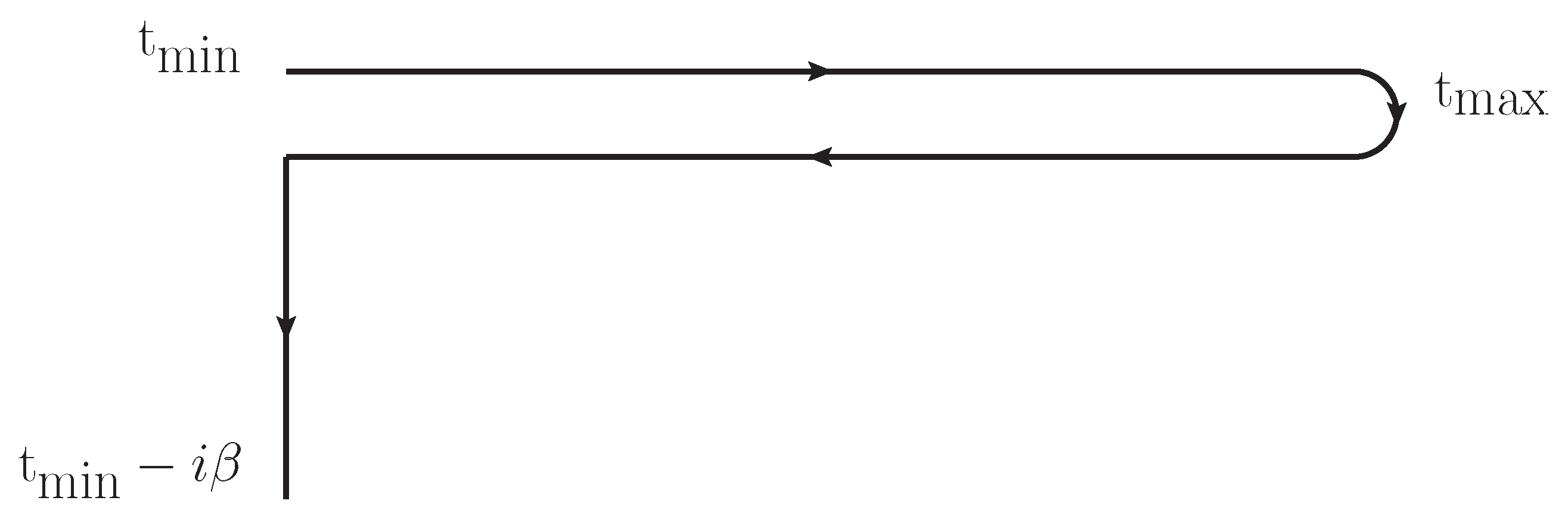
The analysis of the two-time Green’s function is done on the Keldysh contour, illustrated in Figure 1. The imaginary spur allows for the calculation of an equilibrium thermal state at $t_{\min }$, which is subsequently propagated forward in time along the contour using the equations of motion discussed below. For convenience, we will assume $t_{\min }=0$. The system is then subjected to an external perturbation (a field) at some time $t>0$.

The Green’s function for a state with quasi-momentum $\mathbf{k}$ is defined on the contour as

$$\begin{array}{c}\hfill G_{\mathbf{k}}^{\mathcal{C}}(t,t^{\prime })=-i\langle {\mathcal{T}}_{\mathcal{C}}{\widehat{c}}_{\mathbf{k}}\left(t\right){\widehat{c}}_{\mathbf{k}}^{†}\left(t^{\prime }\right)\rangle ,\end{array}$$

(1)

where ${\mathcal{T}}_{\mathcal{C}}$ is the contour time ordering operator, and ${\widehat{c}}_{\mathbf{k}}^{†}/{\widehat{c}}_{\mathbf{k}}$ are the usual creation and annihilation operators. The superscript $\mathcal{C}$ denotes a contour-ordered quantity. As discussed in Ref. [13], the Green’s function satisfies the equation of motion on the Keldysh contour:

$$\begin{array}{c}\hfill \left[i{\partial }_t-{ϵ}_{\mathbf{k}}\left(t\right)\right]G_{\mathbf{k}}^{\mathcal{C}}(t,t^{\prime })={\delta }^{\mathcal{C}}(t,t^{\prime })+{\int }_{\mathcal{C}}{\mathsf{\Sigma }}^{\mathcal{C}}(t,\overline{t})G_{\mathbf{k}}^{\mathcal{C}}(\overline{t},t^{\prime })d\overline{t},\end{array}$$

(2)

as well as a similar (adjoint) equation for $t^{\prime }$. Here, the integration is carried out over the entire contour. Σ encodes the interactions in a diagrammatic sense, and is a functional of the Green’s function. For simplicity, we have chosen a momentum-independent self-energy.

Based on the location of the two times, we can break up the contour-ordered Green’s function into different temporal components. The real-time Green’s functions are the lesser, greater, retarded, and advanced components (<, >, R, and A). They are related through:

$$\begin{array}{cc}\hfill G_{\mathbf{k}}^{<}(t,t^{\prime })& =G_{\mathbf{k}}^{\mathcal{C}}(t\text{on}\text{upper}\text{real}\text{branch},t^{\prime }\text{on}\text{lower}\text{real}\text{branch}),\hfill \end{array}$$

(3)

$$\begin{array}{cc}\hfill G_{\mathbf{k}}^{>}(t,t^{\prime })& =G_{\mathbf{k}}^{\mathcal{C}}(t\text{on}\text{lower}\text{real}\text{branch},t^{\prime }\text{on}\text{upper}\text{real}\text{branch}),\hfill \end{array}$$

(4)

$$\begin{array}{cc}\hfill G_{\mathbf{k}}^R(t,t^{\prime })& =\theta (t-t^{\prime })\left[G_{\mathbf{k}}^{>}(t,t^{\prime })-G_{\mathbf{k}}^{<}(t,t^{\prime })\right],\hfill \end{array}$$

(5)

$$\begin{array}{cc}\hfill G_{\mathbf{k}}^A(t,t^{\prime })& =-\theta (t^{\prime }-t)\left[G_{\mathbf{k}}^{>}(t,t^{\prime })-G_{\mathbf{k}}^{<}(t,t^{\prime })\right].\hfill \end{array}$$

(6)

The mixed components, when one of the arguments (τ) is on the imaginary spur, and the other (t) on the real time branch, are denoted as $G^{\rceil }(t,\tau )$ and $G^{\lceil }(\tau ,t)$. Finally, the component which has both arguments on the imaginary spur is the usual Matsubara Green’s function $G^M(\tau ,{\tau }^{\prime })$. These subdivisions are applied for all contour-ordered quantities.

We can carry this through for the equation of motion, which splits into 3 distinct pieces, and similarly for the adjoint equation. For completeness, we list them here, following the notation of Ref. [13]. Since time-translation invariance applies on the imaginary axis, the equation of motion is significantly simplified:

$$\begin{array}{c}\hfill \left[-{\partial }_{\tau }-{ϵ}_{\mathbf{k}}\left(0\right)\right]G_{\mathbf{k}}^M\left(\tau \right)=\delta \left(\tau \right)+{\int }_0^{\beta }{\mathsf{\Sigma }}^M(\tau -\overline{\tau })G_{\mathbf{k}}^M\left(\overline{\tau }\right)d\overline{\tau }.\end{array}$$

(7)

The lack of dependence on the real time integrations is a reflection of causality—the equilibrium state on the imaginary spur should not depend on any quantities that occur later in time. The equations involving real times are:

$$\begin{array}{cc}\hfill \left[i\overrightarrow{{\partial }_t}-{ϵ}_{\mathbf{k}}\left(t\right)\right]G_{\mathbf{k}}^{\gtrless }(t,t^{\prime })& =I_{1,\mathbf{k}}^{\gtrless }(t,t^{\prime }),\hfill \end{array}$$

(8)

$$\begin{array}{cc}\hfill G_{\mathbf{k}}^{\gtrless }(t,t^{\prime })\left[-i\overleftarrow{{\partial }_{t^{\prime }}}-{ϵ}_{\mathbf{k}}\left(t^{\prime }\right)\right]& =I_{2,\mathbf{k}}^{\gtrless }(t,t^{\prime }),\hfill \end{array}$$

(9)

$$\begin{array}{cc}\hfill \left[i\overrightarrow{{\partial }_t}-{ϵ}_{\mathbf{k}}\left(t\right)\right]G_{\mathbf{k}}^{\rceil }(t,\tau )& =I_{1,\mathbf{k}}^{\rceil }(t,\tau ),\hfill \end{array}$$

(10)

$$\begin{array}{cc}\hfill G_{\mathbf{k}}^{\lceil }(\tau ,t)\left[-i\overleftarrow{{\partial }_t}-{ϵ}_{\mathbf{k}}\left(t^{\prime }\right)\right]& =I_{2,\mathbf{k}}^{\lceil }(\tau ,t),\hfill \end{array}$$

(11)

where the derivative applies following the direction of the arrow. The terms on the right hand side are the scattering integrals, which we will focus on:

$$\begin{array}{cc}\hfill I_{1,\mathbf{k}}^{\gtrless }(t,t^{\prime })& ={\int }_0^{t}d\overline{t}{\mathsf{\Sigma }}^R(t,\overline{t})G_{\mathbf{k}}^{\gtrless }(\overline{t},t)+{\int }_0^{t^{\prime }}d\overline{t}{\mathsf{\Sigma }}^{\gtrless }(t,\overline{t})G_{\mathbf{k}}^A(\overline{t},t)+\frac{1}{i}{\int }_0^{\beta }d\overline{\tau }{\mathsf{\Sigma }}^{\rceil }(t,\overline{\tau })G_{\mathbf{k}}^{\lceil }(\overline{\tau },t),\hfill \end{array}$$

(12)

$$\begin{array}{cc}\hfill I_{2,\mathbf{k}}^{\gtrless }(t,t^{\prime })& ={\int }_0^{t}d\overline{t}{G}_{\mathbf{k}}^R(t,\overline{t}){\mathsf{\Sigma }}^{\gtrless }(\overline{t},t)+{\int }_0^{t^{\prime }}d\overline{t}{G}_{\mathbf{k}}^{\gtrless }(t,\overline{t}){\mathsf{\Sigma }}^A(\overline{t},t)+\frac{1}{i}{\int }_0^{\beta }d\overline{\tau }{G}_{\mathbf{k}}^{\rceil }(t,\overline{\tau }){\mathsf{\Sigma }}^{\lceil }(\overline{\tau },t),\hfill \end{array}$$

(13)

$$\begin{array}{cc}\hfill I_{\mathbf{k}}^{\lceil }(t,\tau )& ={\int }_0^{t}d\overline{t}{\mathsf{\Sigma }}^R(t,\overline{t})G^{\lceil }(\overline{t},\tau )+\frac{1}{i}{\int }_0^{\beta }d\overline{\tau }{\mathsf{\Sigma }}^{\lceil }(t,\overline{\tau })G_{\mathbf{k}}^M(\overline{\tau }-\tau ),\hfill \end{array}$$

(14)

$$\begin{array}{cc}\hfill I_{\mathbf{k}}^{\rceil }(\tau ,t)& ={\int }_0^{t}d\overline{t}{G}^{\rceil }(\tau ,\overline{t}){\mathsf{\Sigma }}^A(\overline{t},t)+\frac{1}{i}{\int }_0^{\beta }d\overline{\tau }{G}_{\mathbf{k}}^M(\tau -\overline{\tau }){\mathsf{\Sigma }}^{\rceil }(\overline{\tau },t).\hfill \end{array}$$

(15)

The scattering integrals have two distinct sets of terms: those involving values on the imaginary axis, and those that do not. In the presence of any type of interactions, the Green’s functions decay in the $t-t^{\prime }$ direction. This leads to a decay in the contribution of the mixed pieces to the integrals as time gets further from $t=0$. We will assume that t and $t^{\prime }$ have advanced sufficiently far from $t=t^{\prime }=0$ that we can neglect those mixed pieces in our analysis.

The density for momentum $\mathbf{k}$ is given by the time-diagonal piece of the lesser Green’s function, $n_{\mathbf{k}}\left(t\right)=-i{G}_{\mathbf{k}}^{<}(t,t)$. To propagate along the $t=t^{\prime }$ ($t_{\mathrm{ave}}$) direction, we need to combine Equations (8) and (9). This yields

$$\begin{array}{cc}\hfill i{\partial }_t{G}_{\mathbf{k}}^{<}(t,t)& =\left[{ϵ}_{\mathbf{k}}\left(t\right),G_{\mathbf{k}}^{<}(t,t)\right]+I_{1,\mathbf{k}}^{<}(t,t)-I_{2,\mathbf{k}}^{<}(t,t),\hfill \end{array}$$

(16)

which can be simplified by noting that $I_{1,\mathbf{k}}^{\gtrless }(t,t^{\prime })=-I_{2,\mathbf{k}}^{\gtrless }{(t^{\prime },t)}^{†}$. For single-band models on lattices without a basis the Green’s function can be described by a set of scalars and the energy ${ϵ}_{\mathbf{k}}\left(t\right)$ commutes with the Green’s function. We can further assume that we have gone far enough along in t and $t^{\prime }$ that we can extend the lower bound of the integral to $-\infty$ due to the Green’s function decay, and are left with:

$$\begin{array}{cc}\hfill i{\partial }_t{G}_{\mathbf{k}}^{<}(t,t)={\int }_{-\infty }^{t}d\overline{t}& \left\{{\mathsf{\Sigma }}^R(t,\overline{t})G_{\mathbf{k}}^{<}(\overline{t},t)+{\mathsf{\Sigma }}^{<}(t,\overline{t})G_{\mathbf{k}}^A(\overline{t},t)\right.\hfill \\ & \left.-G_{\mathbf{k}}^{<}(t,\overline{t}){\mathsf{\Sigma }}^A(\overline{t},t)-G_{\mathbf{k}}^R(t,\overline{t}){\mathsf{\Sigma }}^{<}(\overline{t},t)\right\},\hfill \\ \hfill \equiv {\mathsf{\Sigma }}^R·G_{\mathbf{k}}^{<}& +{\mathsf{\Sigma }}^{<}·G_{\mathbf{k}}^A-G_{\mathbf{k}}^{<}·{\mathsf{\Sigma }}^A-G_{\mathbf{k}}^R·{\mathsf{\Sigma }}^{<},\hfill \end{array}$$

(17)

where in the last line we have introduced the · (as a non-Abelian operator) to represent the integral for notational convenience.

2.2. General Remarks on the Scattering Integrals

It is instructive to consider the contour-ordered quantities as functions of the average and relative time, rather than the explicit t and $t^{\prime }$: $t_{\mathrm{ave}}=\frac{1}{2}\left(t+t^{\prime }\right),t_{\mathrm{rel}}=t-t^{\prime }$. The population dynamics occurs along the $t_{\mathrm{ave}}$ direction, whereas quasiparticle lifetimes arise from the $t_{\mathrm{rel}}$ direction. The scattering integrals control the temporal dynamics of the Green’s function along the $t_{\mathrm{ave}}$ direction. Thus, an examination of the integrals can lead to some general insights regarding the dynamics. First, it can be shown that an average time dependence is necessary for any change to occur—that is, without any dependence on $t_{\mathrm{ave}}$, the scattering integrals (and thus the time derivative of the density) are 0.

It is illustrative to consider the equations in a form where the Fourier transform over $t_{\mathrm{rel}}$ has been performed. For this transform to be well-defined, we must assume that any average time dependence is slow enough within the window of Fourier transformation set by the decay of the Green’s function along $t_{\mathrm{rel}}$ that we can replace the average time dependence with a single time only, namely $t_{\mathrm{ave}}$. Any applied field is assumed to have occurred sufficiently far in the past that it falls outside this window. This yields

$$\begin{array}{cc}\hfill i{\partial }_{t_{\mathrm{ave}}}{G}_{\mathbf{k}}^{<}(t_{\mathrm{ave}},\omega )& =2i\mathrm{Im}\left[{\mathsf{\Sigma }}^R(t_{\mathrm{ave}},\omega )\right]G_{\mathbf{k}}^{<}(t_{\mathrm{ave}},\omega )\hfill \\ & -2i\mathrm{Im}\left[G_{\mathbf{k}}^R(t_{\mathrm{ave}},\omega )\right]{\mathsf{\Sigma }}^{<}(t_{\mathrm{ave}},\omega ).\hfill \end{array}$$

(18)

When there is no dependence on $t_{\mathrm{ave}}$, we can use Dyson’s equation and substitute for $G_{\mathbf{k}}^{<}\left(\omega \right)$ and $\mathrm{Im}{G}_{\mathbf{k}}^R\left(\omega \right)$. Long after $t=t^{\prime }=0$ where the mixed components have decayed, we can re-write Dyson’s equation (Equations (8) and (12)) in the following way:

$$\begin{array}{cc}\hfill G_{\mathbf{k}}^{<}& =G_{\mathbf{k}}^R·{\mathsf{\Sigma }}^{<}·G_{\mathbf{k}}^A.\hfill \end{array}$$

(19)

Making the same transformation to $t_{\mathrm{ave}},t_{\mathrm{rel}}$ and Fourier transforming over $t_{\mathrm{rel}}$, we can substitute this result into Equation (19):

$$\begin{array}{cc}\hfill i{\partial }_{t_{\mathrm{ave}}}{G}^{<}(t_{\mathrm{ave}},\omega )& =2i\mathrm{Im}\left[{\mathsf{\Sigma }}^R(t_{\mathrm{ave}},\omega )\right]{\mathsf{\Sigma }}^{<}(t_{\mathrm{ave}},\omega ){\left|G_{\mathbf{k}}^R(t_{\mathrm{ave}},\omega )\right|}^2\hfill \\ & -2i\mathrm{Im}\left[{\mathsf{\Sigma }}^R(t_{\mathrm{ave}},\omega )\right]{\left|G_{\mathbf{k}}^R(t_{\mathrm{ave}},\omega )\right|}^2{\mathsf{\Sigma }}^{<}(t_{\mathrm{ave}},\omega )\hfill \\ & =0.\hfill \end{array}$$

(20)

The point here is that the lack of time dependence in the density comes from the cancellation of two terms, rather than each term being 0 individually. This will come up again when we consider specific cases.

The central result is even stronger than this: once the lesser Green’s function can be represented by any distribution function of average time and frequency that multiplies the imaginary part of the retarded Green’s function at the same average time and frequency, that is $G_{\mathbf{k}}^{<}(t_{\mathrm{ave}},\omega )=-2i{f}_{\text{dist}}(t_{\mathrm{ave}},\omega )\mathrm{Im}{G}_{\mathbf{k}}^R(t_{\mathrm{ave}},\omega )$ (and similar for the self-energy), then the population no longer changes with time. The factor of two arises from the connection to equilibrium; this assumption is true if the system has equilibriated at an elevated temperature $T_{el}$, where the fluctuation-dissipation theorem holds and $f(\omega ,T_{el})$ is the Fermi function. We can readily see this from Equation (19) by substituting this relation:

$$\begin{array}{cc}\hfill i{\partial }_{t_{\mathrm{ave}}}{G}_{\mathbf{k}}^{<}(t_{\mathrm{ave}},\omega )& =4\mathrm{Im}\left[{\mathsf{\Sigma }}^R(t_{\mathrm{ave}},\omega )\right]f_{\text{dist}}(t_{\mathrm{ave}},\omega )\mathrm{Im}{G}_{\mathbf{k}}^R(t_{\mathrm{ave}},\omega )\hfill \\ & -4\mathrm{Im}\left[G^R(t_{\mathrm{ave}},\omega )\right]f_{\text{dist}}(t_{\mathrm{ave}},\omega )\mathrm{Im}{\mathsf{\Sigma }}^R(t_{\mathrm{ave}},\omega )\hfill \\ & =0.\hfill \end{array}$$

(21)

Note that this cancellation occurs for all types of scattering and for all strengths of the scattering. It does not require any so-called "bottlenecks" but simply follows from the dynamics of the populations and the exact form of the scattering integral. A further implication of this cancellation is that a simple hot electron model cannot fully describe the dynamics because approximating $G_{\mathbf{k}}^{<}(t_{\mathrm{ave}},\omega )$ and ${\mathsf{\Sigma }}^{<}(t_{\mathrm{ave}},\omega )$ by the retarded components multiplied by the same average-time dependent distribution function will not work, because such systems do not evolve in time any further, even though the distributions are different from the equilibrium distributions.

2.2.1. Self-Consistency

A point should be raised here regarding self-consistency—that is, using the density after the pump to determine the self-energy, rather than using the equilibrium density. This is equivalent to using the unrenormalized Green’s function to evaluate the self-energy, which is often done in equilibrium approaches to evaluate first-order effects. As we will show, this is not the same in the time domain. Without self-consistency, the above approach cannot be applied in the same fashion because the relation between Σ and $G_{\mathbf{k}}$ is not as clear. Instead, as above, let us assume that some time after the pump, the system can be described as a population occupying an equilibrium spectral function—that is, $G_{\mathbf{k}}^{<}(t_{\mathrm{ave}},\omega )=-2i{f}_{\text{dist}}(t_{\mathrm{ave}},\omega )\mathrm{Im}{G}_{\mathbf{k},\text{eq}}^R\left(\omega \right)$. Then, if the self-energy is given by the original equilibrium one, we find

$$\begin{array}{cc}\hfill i{\partial }_{t_{\mathrm{ave}}}{G}_{\mathbf{k}}^{<}(t_{\mathrm{ave}},\omega )& =4\mathrm{Im}\left[{\mathsf{\Sigma }}^R\left(\omega \right)\right]\mathrm{Im}\left[G_{\mathbf{k},\text{eq}}^R\left(\omega \right)\right]\left[f_{\text{dist}}(t_{\mathrm{ave}},\omega )-f_{\text{eq}}\left(\omega \right)\right],\hfill \end{array}$$

(22)

where $f_{\text{eq}}\left(\omega \right)$ is the equilibrium distribution used to evaluate self-energy. If the self-energy is thus determined based on the equilibrium Green’s functions, there cannot be a balance of terms and the density will decay until it reaches the initial equilibrium state, independent of the types of interactions present. More generally, if the distribution is the same for $G_{\mathbf{k}}^{<}(t_{\mathrm{ave}},\omega )$ as for ${\mathsf{\Sigma }}^{<}\left(\omega \right)$, then there is no further relaxation.

One way this can be further understood is by breaking the self-energy into “dark” and “induced” pieces, following the work by S̆pic̆ka et al. [14,15,16]. Starting from Equation (18) we find

$$\begin{array}{c}\hfill i{\partial }_{t_{\mathrm{ave}}}{G}_{\mathbf{k}}^{<}(t_{\mathrm{ave}},\omega )={\mathsf{\Sigma }}_D^R·G_{\mathbf{k}}^{<}-{\mathsf{\Sigma }}_D^{<}·G_{\mathbf{k}}^A+{\mathsf{\Sigma }}_I^R·G_{\mathbf{k}}^{<}-{\mathsf{\Sigma }}_I^{<}·G_{\mathbf{k}}^A+\mathrm{H}.\mathrm{C}.\end{array}$$

(23)

At this point, we can identify the first two terms on the RHS as those captured by approaches lacking self-consistency—they capture the changes in the Green’s function, but not the self-energy. If we limit the RHS to these terms and apply the approach discussed above, it becomes clear how the population dynamics have a simple connection to the equilibrium (or “dark”) retarded self-energy:

$$\begin{array}{cc}\hfill i{\partial }_{t_{\mathrm{ave}}}{G}_{\mathbf{k}}^{<}(t_{\mathrm{ave}},\omega )& =4\mathrm{Im}\left[{\mathsf{\Sigma }}_D^R\left(\omega \right)\right]\mathrm{Im}\left[G_{\mathbf{k},D}^R\left(\omega \right)\right]\left[f(t_{\mathrm{ave}},\omega )-f_{eq}\left(\omega \right)\right]\hfill \\ & =-2i\mathrm{Im}\left[{\mathsf{\Sigma }}_D^R\left(\omega \right)\right]G_{\mathbf{k},I}^{<}(t_{\mathrm{ave}},\omega ).\hfill \end{array}$$

(24)

As long as the induced density is different from 0, we can observe a decay with an exponential decay constant $\tau {\left(\omega \right)}^{-1}=-2\mathrm{Im}{\mathsf{\Sigma }}_D^R\left(\omega \right)$. This is the relation between the population decay and self-energy reported previously [5,17]. It is the same relation as that between the decay of the Green’s function in relative time $t_{\mathrm{rel}}$, but does not have the same origin. In that case, the self-energy gives rise to a line width in the spectrum of a single excitation, as measured, e.g., by equilibrium photoemission spectroscopy. Here, the relation arrives only through copious approximations applied to population dynamics [14,15,16], which occur along an orthogonal direction to $t_{\mathrm{rel}}$. We require the population dynamics to be very slow for this to hold, or for the pump-induced population changes to be extremely small such that only these terms play a role. Once the approximations are violated, more complex dynamics arise, as discussed by several authors [6,13,18,19]. This can already be seen from Equation (22), which bears a remarkable similarity to Equation (24) except that the full pump-modified self-energy has to be accounted for. This leads to modification of the observed interactions by the pump, as discussed in [6,20,21].

Evidently, the lack of self-consistency is an uncontrolled approximation in the time domain, which can fail to capture important aspects of the population dynamics such as predicting the wrong decay rates and a return to equilibrium when the scattering process cannot dissipate energy.

2.2.2. Specific Examples

As a concrete illustration of the above, let us consider a simple form of impurity scattering which can account for the changes in the density due to the pump: the self-consistent Born approximation, where the self-energy is proportional to the local Green’s function: ${\mathsf{\Sigma }}^R(t,t^{\prime })=V^2{\sum }_{\mathbf{k}}{G}_{\mathbf{k}}^R(t,t^{\prime })$, and similarly for the other Keldysh components. Inserting this into Equation (18), and applying the equations above, we find

$$\begin{array}{cc}\hfill i{\partial }_{t_{\mathrm{ave}}}{G}_{\mathbf{k}}^{<}(t,t)& =V^2\sum _{\mathbf{p}}\left[G_{\mathbf{p}}^R·G_{\mathbf{k}}^{<}+G_{\mathbf{p}}^{<}·G_{\mathbf{k}}^A-G_{\mathbf{k}}^{<}·G_{\mathbf{p}}^A-G_{\mathbf{k}}^R·G_{\mathbf{p}}^{<}\right]\hfill \end{array}$$

(25)

$$\begin{array}{cc}\hfill i{\partial }_{t_{\mathrm{ave}}}{G}_{\mathbf{k}}^{<}(t_{\mathrm{ave}},\omega )& =2i{V}^2\sum _{\mathbf{p}}\left\{\mathrm{Im}\left[G_{\mathbf{p}}^R(t_{\mathrm{ave}},\omega )\right]G_{\mathbf{k}}^{<}(t_{\mathrm{ave}},\omega )-\mathrm{Im}\left[G_{\mathbf{k}}^R(t_{\mathrm{ave}},\omega )\right]G_{\mathbf{p}}^{<}(t_{\mathrm{ave}},\omega )\right\}\hfill \\ & \approx 2i{V}^2\sum _{\mathbf{p}}\mathrm{Im}\left[G_{\mathbf{p}}^R\left(\omega \right)\right]\mathrm{Im}\left[G_{\mathbf{k}}^R\left(\omega \right)\right]\left\{f(t_{\mathrm{ave}},\omega )-f(t_{\mathrm{ave}},\omega )\right\}\hfill \\ \hfill & =0.\hfill \end{array}$$

(26)

This is a particularly striking result in light of the usual equilibrium connection between the quasiparticle lifetime and the self-energy. Here, the self-energy is clearly finite, whether calculated based on the pumped states or the equilibrium states, yet the population decay rate is 0 once the system has reached a state where the distribution function is independent of momentum.

As a final note, we may apply the above methodology to a system of purely interacting electrons. The lowest-order term that leads to scattering of more than 1 electron is at 2nd order, with

$$\begin{array}{c}\hfill {\mathsf{\Sigma }}_{\mathbf{k}}^{\mathcal{C}}(t,t^{\prime })=\sum _{\mathbf{q}\mathbf{p}}{U}_{\mathbf{q}}{G}_{\mathbf{k}-\mathbf{q}}^{\mathcal{C}}(t,t^{\prime })G_{\mathbf{p}}^{\mathcal{C}}(t,t^{\prime })G_{\mathbf{p}+\mathbf{q}}^{\mathcal{C}}(t,t^{\prime }).\end{array}$$

(27)

Although the algebra is more complex, it can nevertheless be shown that once the electrons have been approximated as a thermal distribution occupying the spectral function, the RHS of the equations of motion are identically 0. This is as expected, since a thermalized state is the stable solution for a system of interacting electrons. Indeed, the specific form of the scattering mechanism is not important, the dependence of the lesser quantities on the distribution function is the important element.

The conventional “hot-electron” viewpoint, where the electrons rapidly relax to a Fermi-Dirac distribution at high temperature which then cools down to a low temperature Fermi-Dirac distribution, cannot take place in this fashion. Once the system is described by a quasi-equilibrium distribution function, it will no longer relax.

2.3. Numerical Evaluation of the Scattering Integrals

To evaluate the approximations and confirm the arguments made above, we perform numerical evaluation of the equations of motion on the Keldysh contour. The method has been described in some detail in Refs. [6,13]. We will follow the same separation used and motivated in the previous section, and consider separately the terms $I_{\mathbf{k}}^{\mathsf{\Sigma }}\equiv {\mathsf{\Sigma }}^R·G_{\mathbf{k}}^{<}-G_{\mathbf{k}}^{<}·{\mathsf{\Sigma }}^A$ and $I_{\mathbf{k}}^G\equiv G_{\mathbf{k}}^R·{\mathsf{\Sigma }}^{<}-{\mathsf{\Sigma }}^{<}·G_{\mathbf{k}}^A$. These are different from $I_{\mathbf{k}}^1$ and $I_{\mathbf{k}}^2$, but rather are the full scattering integral separated into the terms that lead to two terms as they appear in Equation (19). As noted above, these two terms should balance when there is no further time dependence to the density. The full scattering integral is then a difference between the two (see Equation (18)).

As an illustrative model, we choose the Holstein-Hubbard Hamiltonian with local scattering:

$$\begin{array}{c}\hfill \mathcal{H}=\sum _{\mathbf{k},\sigma }{ϵ}_{\mathbf{k}}{\widehat{c}}_{\mathbf{k},\sigma }^{†}{\widehat{c}}_{\mathbf{k},\sigma }+U\sum _i{\widehat{n}}_{i\uparrow }{\widehat{n}}_{i\downarrow }+g\sum _{k,q,\sigma }{\widehat{c}}_{k+q,\sigma }^{†}{\widehat{c}}_{k,\sigma }\left({\widehat{b}}_q+{\widehat{b}}_{-q}^{†}\right)+\mathsf{\Omega }\sum _i\left({\widehat{b}}_i^{†}{\widehat{b}}_i+\frac{1}{2}\right),\end{array}$$

(28)

where ${\widehat{c}}^{†}/\widehat{c}$ and ${\widehat{b}}^{†}/\widehat{b}$ are the creation and annihilation operators for electrons and phonons, respectively, and ${\widehat{n}}_i\equiv {\widehat{c}}_i^{†}{\widehat{c}}_i$ is the local density operator.

The electron-electron interactions are treated at second order, with

$$\begin{array}{c}\hfill {\mathsf{\Sigma }}_{\mathrm{e}-\mathrm{e}}^{\mathcal{C}}(t,t^{\prime })=U^2{G}_{\mathrm{local}}^{\mathcal{C}}(t,t^{\prime })\star G_{\mathrm{local}}^{\mathcal{C}}(t,t^{\prime })\star G_{\mathrm{local}}^{\mathcal{C}}(t^{\prime },t)\end{array}$$

(29)

where the star (⋆) denotes a product on the Keldysh contour. When present, $U^2=0.09$ eV${}^2$. The electron-phonon scattering is treated at first order within the Migdal-Eliashberg formalism, with

$$\begin{array}{c}\hfill {\mathsf{\Sigma }}_{\mathrm{e}-\mathrm{p}}^{\mathcal{C}}(t,t^{\prime })=g^2{G}_{\mathrm{local}}^{\mathcal{C}}(t,t^{\prime })\star D_0^{\mathcal{C}}(t,t^{\prime }),\end{array}$$

(30)

where $D_0^{\mathcal{C}}(t,t^{\prime })$ is the propagator for a bare Einstein phonon with frequency Ω. When present, $g^2=0.01$ eV${}^2$ and $\mathsf{\Omega }=0.2$ eV. We employ a two-dimensional tight-binding model with nearest neighbor hopping $V_{\mathrm{nn}}=0.25$ eV and a chemical potential $\mu =-0.2$ eV. The field is applied using minimal coupling in the Hamiltonian gauge. We use a simple oscillatory field in the zone diagonal ($k_x=k_y$) direction with $A\left(t\right)=A_{\max }sin\left(\omega t\right)exp(-\frac{1}{2}{(t-t_0)}^2/{\sigma }^2)$, where $\omega =0.5$ eV, $t_0=60$ eV${}^{-1}$, $\sigma =10$ eV${}^{-1}$ and $A_{\max }=0.8$.

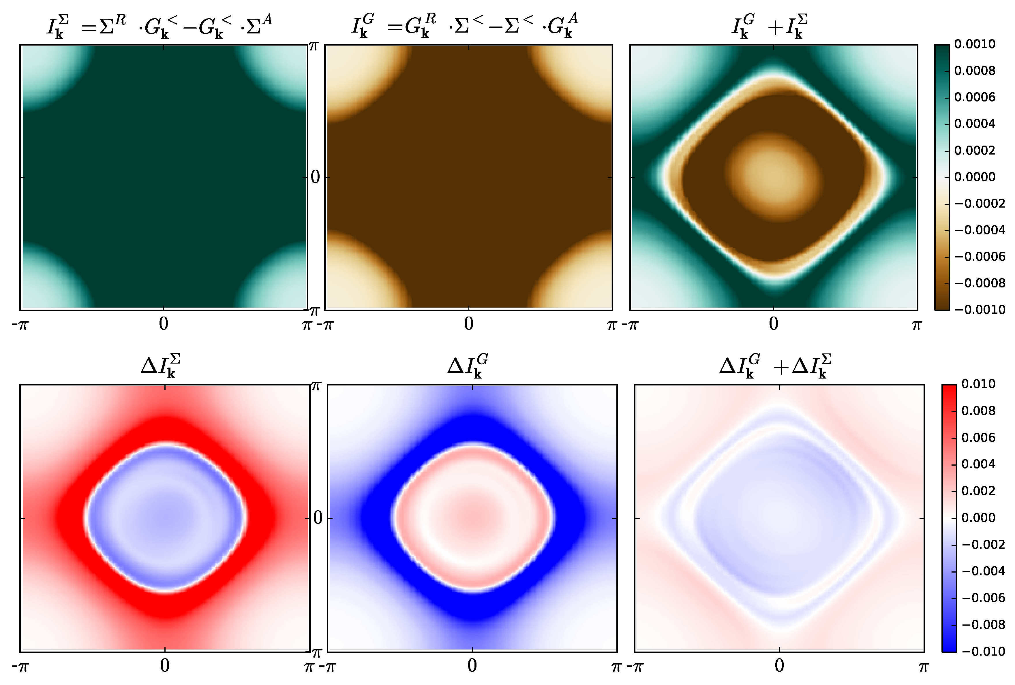
Figure 2 shows the scattering integrals for a case with both types of scattering (e-e and e-p) at $t=108$ after the pump. The separated terms $I_{\mathbf{k}}^{\mathsf{\Sigma }}$ and $I_{\mathbf{k}}^G$ are both large and appear featureless on these scales, while their sum has some definite structure. To elucidate this further, we consider the difference from equilibrium, $\Delta I_{\mathbf{k}}^{\mathsf{\Sigma }}$ and $\Delta I_{\mathbf{k}}^G$, shown in the bottom row of Figure 2. The pump has clearly induced a difference from the equilibrium scattering integrals, giving an average time dependence to the self-energy and Green’s functions and thus resulting in a finite summed scattering rate. There is some momentum dependence to the terms, although the details of the momentum dependence can vary based on the types of scattering present and their amplitudes. As time goes on, the system will reach some steady state where it has either returned to its equilibrium state (where $\Delta I_{\mathbf{k}}^{\mathsf{\Sigma }}$ and $\Delta I_{\mathbf{k}}^G$ also go to 0) or where a new state is achieved, with a finite $\Delta I_{\mathbf{k}}^{\mathsf{\Sigma }}$ and $\Delta I_{\mathbf{k}}^G$ which balance. In the first case, the system is once again thermal (since it started from a thermal state). In the latter case, the system does not have to achieve a thermal state—it is sufficient that ${\mathsf{\Sigma }}^{<}$ and $G^{<}$ are described by the same population distribution. A thermal state also satisfies this, but nonthermal states can as well. In the case we are studying with phonons, the system will approach a thermal state at the temperature of the phonon bath, but other situations may result in nonthermal states since both are naturally possible within the general theory.

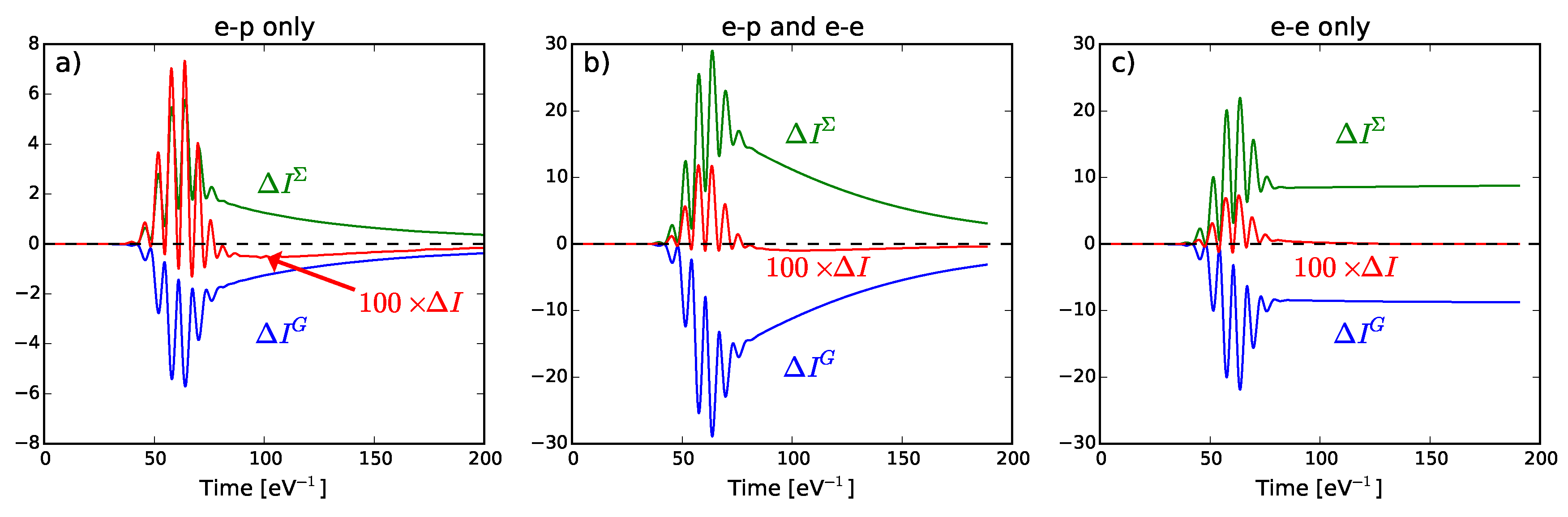
The latter can be achieved in the case of e-e scattering without any further mechanism for removing the energy from the system. These cases can be illustrated by considering the time dependence of $\Delta I^{\mathsf{\Sigma },G}\equiv {\sum }_{\mathbf{k}}\Delta I_{\mathbf{k}}^{\mathsf{\Sigma },G}$. Figure 3 shows the time traces of momentum-summed $\Delta I^{\mathsf{\Sigma }}$ and $\Delta I^G$. When only e-p scattering is present, the system behaves essentially as expected and reported previously [6] with an exponential, slow return to equilibrium together with a slow decrease of both scattering integrals. The sum also goes to zero on a similar time scale. It should be noted that the magnitude of $\Delta I$ is much smaller than the two contributions $\Delta I^{\mathsf{\Sigma },G}$, confirming again that the balance between terms controls the dynamics. As e-e scattering is introduced, more energy is absorbed during the pump and the scale of the changes increases, but the salient features remain the same.

Finally, when e-p scattering is not present, a markedly different scenario occurs. The scattering integrals remain different from their equilibrium values, but as the system relaxes, they lose their average time dependence and balance out to give a net sum of 0 at long times. In this particular case, the state reflects a “thermalized” electron system, where the scattering has taken place until a balance (reflected in a Fermi distribution) is achieved. However, as noted above, the balance is not limited to thermalized states. It can also be achieved with a non-thermal electron distribution, so long as the same distribution is used in determining the self-energy.

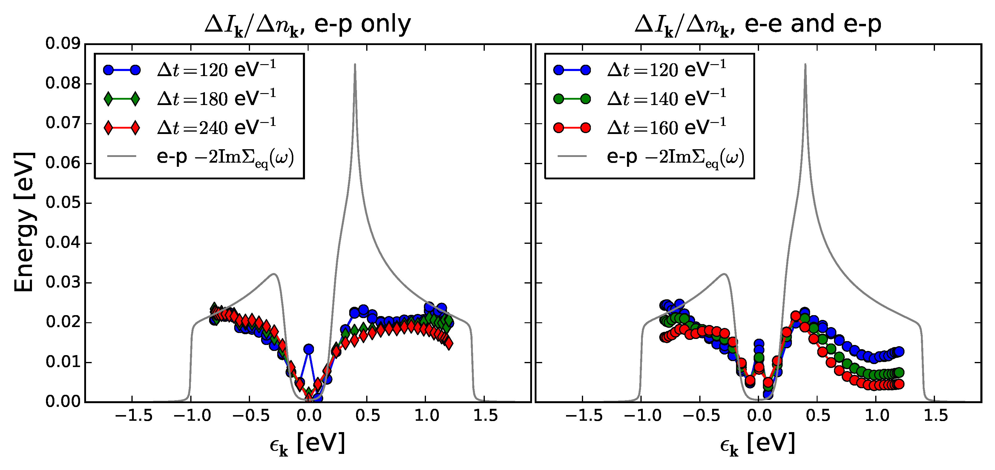
To further illustrate the importance of cancellation between $\Delta I^{\mathsf{\Sigma }}$ and $\Delta I^G$, we can estimate the decay constant by considering the ratio

$$\begin{array}{c}\hfill \frac{\Delta I_{\mathbf{k}}}{\Delta n_{\mathbf{k}}}=i\frac{\Delta I_{\mathbf{k}}^{\mathsf{\Sigma }}+\Delta I_{\mathbf{k}}^G}{G_{\mathbf{k}}^{<}(t,t)-G_{\mathbf{k}}^{<}(0,0)}.\end{array}$$

(31)

In the weak pumping limit this is approximately equal to $-2\mathrm{Im}\mathsf{\Sigma }(\omega ={ϵ}_{\mathbf{k}})$. The approximate relation becomes exact if self-consistency is neglected. For e-p scattering only, $\Delta I_{\mathbf{k}}/\Delta n_{\mathbf{k}}$ shows a reasonable agreement with the equilibrium self-energy, although some deviation is present and in fact expected because we know that there is a contribution from the $\Delta I^G$ term in the scattering integrals. Nevertheless, the step in the scattering rate near the phonon frequency is recognizable. Since the scattering integral $\Delta I$ does not show any signs of a balance before the full decay, we observe that $\Delta I_{\mathbf{k}}/\Delta n_{\mathbf{k}}$ remains relatively constant at early times. When e-e scattering is included, a competition between the scattering mechanisms arises that leads to a mismatch between $1/\tau$ and $-2\mathrm{Im}{\mathsf{\Sigma }}_{\mathrm{eq}}(\omega ={ϵ}_{\mathbf{k}}))$ [22]. This is reflected in the scattering integrals as a deviation from simple exponential decay, and a time dependence in $\Delta I_{\mathbf{k}}/\Delta n_{\mathbf{k}}$. Although the phonon window can still be observed as the energy dissipation of the system is governed by the e-p process, the exact connection to the equilibrium self-energy is rapidly lost as the e-e scattering modifies the relaxation of the system so that the electrons only thermalize when they reach the phonon temperature.

3. Discussion

We have considered a few aspects of the equations of motion for the population of an excited system. The major result is that a nontrivial average time dependence of the Green’s function and self-energy is needed to have any population dynamics at all, and that a steady state is reached when there is a balance of scattering integrals after excitation rather than a full return to equilibrium of the same. Approximating the system with a hot electron model cannot capture the dynamics, as it was shown to lead to an exact cancellation of the scattering integrals unless the electrons are coupled to an external bath (e.g., of phonons). To be able to achieve this balance, a full self-consistent treatment (where the self-energy reflects the changed population distribution) is necessary (the self-energy is selfconsistently evaluated as the functional of the full Green’s function as in any conserving approach). This naïvely makes sense because the redistributed population should be accounted for in the interactions, but stands in contrast to equilibrium physics where self-consistency often only gives a correction on top of the major feature obtained in 1st order. For example, the kink and step in the spectral weight due to a strongly coupled boson in Migdal-Eliashberg theory arise readily whether the bare or renormalized electron propagator is used in the calculation of the self-energy. In the time domain, ignoring self-consistency does capture the main feature when the system is solely coupled to an external bath [5,6], but beyond this situation this approach is insufficient. This leads to the conclusion that the relation between the population relaxation rate and the equilibrium self-energy $\tau {(\mathbf{k},\omega )}^{-1}=-2\mathrm{Im}{\mathsf{\Sigma }}_{\mathrm{eq}}(\mathbf{k},\omega )$ only holds exactly in very limited cases for non-equilibrium experiments, although it appears to be approximately true over a much wider range of cases as can be seen in Figure 4.

4. Materials and Methods

The equations of motion for the Green’s function are solved using a predictor-corrector time-stepping algorithm detailed in [13]. The thermal problem is solved on the Matsubara axis, which is followed by a forward time-stepping procedure. At each time step, the self-energy is evaluated and the forward time step is made, followed by a correction step. This is repeated until the Green’s function at the new time is converged, and the algorithm moves on to the next time step.

References

1. Freericks, J.K.; Turkowski, V.M.; Zlatić, V. Nonequilibrium Dynamical Mean-Field Theory. Phys. Rev. Lett. 2006, 97, 266408. [Google Scholar] [CrossRef] [PubMed]
2. Aoki, H.; Tsuji, N.; Eckstein, M.; Kollar, M.; Oka, T.; Werner, P. Nonequilibrium dynamical mean-field theory and its applications. Rev. Mod. Phys. 2014, 86, 779–837. [Google Scholar] [CrossRef]
3. Freericks, J.K.; Krishnamurthy, H.R.; Pruschke, T. Theoretical Description of Time-Resolved Photoemission Spectroscopy: Application to Pump-Probe Experiments. Phys. Rev. Lett. 2009, 102, 136401. [Google Scholar] [CrossRef] [PubMed]
4. Moritz, B.; Kemper, A.F.; Sentef, M.; Devereaux, T.P.; Freericks, J.K. Electron-Mediated Relaxation Following Ultrafast Pumping of Strongly Correlated Materials: Model Evidence of a Correlation-Tuned Crossover between Thermal and Nonthermal States. Phys. Rev. Lett. 2013, 111, 077401. [Google Scholar] [CrossRef] [PubMed]
5. Sentef, M.; Kemper, A.F.; Moritz, B.; Freericks, J.K.; Shen, Z.X.; Devereaux, T.P. Examining Electron-Boson Coupling Using Time-Resolved Spectroscopy. Phys. Rev. X 2013, 3, 041033. [Google Scholar] [CrossRef]
6. Kemper, A.F.; Sentef, M.A.; Moritz, B.; Freericks, J.K.; Devereaux, T.P. Effect of dynamical spectral weight redistribution on effective interactions in time-resolved spectroscopy. Phys. Rev. B 2014, 90, 075126. [Google Scholar] [CrossRef]
7. Eckstein, M.; Werner, P. Photoinduced States in a Mott Insulator. Phys. Rev. Lett. 2013, 110, 126401. [Google Scholar] [CrossRef] [PubMed]
8. Eckstein, M.; Werner, P. Ultrafast Separation of Photodoped Carriers in Mott Antiferromagnets. Phys. Rev. Lett. 2014, 113, 076405. [Google Scholar] [CrossRef] [PubMed]
9. Werner, P.; Held, K.; Eckstein, M. Role of impact ionization in the thermalization of photoexcited Mott insulators. Phys. Rev. B 2014, 90, 235102. [Google Scholar] [CrossRef]
10. Golež, D.; Eckstein, M.; Werner, P. Dynamics of screening in photodoped Mott insulators. Phys. Rev. B 2015, 92, 195123. [Google Scholar] [CrossRef]
11. Eckstein, M.; Werner, P. Ultra-fast photo-carrier relaxation in Mott insulators with short-range spin correlations. Sci. Rep. 2016, 6, 21235. [Google Scholar] [CrossRef] [PubMed]
12. Galitskii, V.M.; Migdal, A.B. Translation: Soviet Phys. JETP 1958, 7, 96–104. [Google Scholar]
13. Stefanucci, G.; van Leeuwen, R. Nonequilibrium Many-Body Theory of Quantum Systems: A Modern Introduction, 1st ed.; Cambridge University Press: Cambridge, UK, 2013. [Google Scholar]
14. Špička, V.; Velický, B.; Kalvová, A. Long and short time quantum dynamics: I. Between Green’s functions and transport equations. Phys. E Low-dimens. Syst. Nanostruct. 2005, 29, 154–174. [Google Scholar] [CrossRef]
15. Špička, V.; Velický, B.; Kalvová, A. Long and short time quantum dynamics: II. Kinetic regime. Phys. E Low-dimens. Syst. Nanostruct. 2005, 29, 175–195. [Google Scholar] [CrossRef]
16. Špička, V.; Velický, B.; Kalvová, A. Long and short time quantum dynamics: III. Transients. Phys. E Low-dimens. Syst. Nanostruct. 2005, 29, 196–212. [Google Scholar] [CrossRef]
17. Kemper, A.F.; Sentef, M.; Moritz, B.; Kao, C.C.; Shen, Z.X.; Freericks, J.K.; Devereaux, T.P. Mapping of unoccupied states and relevant bosonic modes via the time-dependent momentum distribution. Phys. Rev. B 2013, 87, 235139. [Google Scholar] [CrossRef]
18. Marini, A. Competition between the electronic and phonon–domediated scattering channels in the out-of-equilibrium carrier dynamics of semiconductors: An ab-initio approach. J. Phys. Conf. 2013, 427, 012003. [Google Scholar] [CrossRef]
19. Murakami, Y.; Werner, P.; Tsuji, N.; Aoki, H. Interaction quench in the Holstein model: Thermalization crossover from electron- to phonon-dominated relaxation. Phys. Rev. B 2015, 91, 045128. [Google Scholar] [CrossRef]
20. Rameau, J.D.; Freutel, S.; Rettig, L.; Avigo, I.; Ligges, M.; Yoshida, Y.; Eisaki, H.; Schneeloch, J.; Zhong, R.D.; Xu, Z.J.; et al. Photoinduced changes in the cuprate electronic structure revealed by femtosecond time- and angle-resolved photoemission. Phys. Rev. B 2014, 89, 115115. [Google Scholar] [CrossRef]
21. Ishida, Y.; Saitoh, T.; Mochiku, T.; Nakane, T.; Hirata, K.; Shin, S. Quasi-particles ultrafastly releasing kink bosons to form Fermi arcs in a cuprate superconductor. Sci. Rep. 2016, 6, 18747. [Google Scholar] [CrossRef] [PubMed]
22. Rameau, J.D.; Freutel, S.; Sentef, M.A.; Kemper, A.F.; Freericks, J.K.; Avigo, I.; Ligges, M.; Rettig, L.; Yoshida, Y.; Eisaki, H.; et al. Energy dissipation in the time domain governed by bosons in a correlated material. 2015; arXiv:1505.07055. [Google Scholar]
Figure 1. The Keldysh contour used in the analysis below. For convenience, t min is set to equal 0.
Entropy 18 00180 g001
Figure 2. Field-induced changes in the momentum dependent scattering integrals, where t = 100 eV - 1 . The panels show the two individual contributions as well as the difference. Top: absolute values. Bottom: difference from equilibrium. The C 4 symmetry is broken due to the field applied in the k x = k y direction.
Entropy 18 00180 g002
Figure 3. Time traces of the change in the momentum-summed scattering integrals Δ I Σ , G ( t ) for a system with (a) only e-p coupling, (b) both e-e and e-p coupling, and (c) only e-e coupling. Before scaling by 100, the sum Δ I Δ I Σ + Δ I G (red) is nearly indistinguishable from the dashed line along the horizontal axis.
Entropy 18 00180 g003
Figure 4. Δ I k / Δ n k for times Δ t after t = 0 (the pump pulse occurs at t = 60 eV - 1 ). The equilibrium electron-phonon self-energy is shown for reference.
Entropy 18 00180 g004