From Steam Engines to Chemical Reactions: Gibbs’ Contribution to the Extension of the Second Law

Abstract

The present work analyzes the foundations of Gibbs’ thermodynamic equilibrium theory, with the general aim of understanding how the Second Law—as formulated by Clausius in 1865—has been embodied into Gibbs’ formal system and extended to processes involving chemical reactions. We show that Gibbs’ principle of maximal entropy (and minimal energy) is the implicit expression of Clausius’ Second Law. In addition, by making explicit some implicit passages of Gibbs logical path, we provide an original formal justification of Gibbs’ principle. Finally we provide an analysis of how Gibbs’ principle—conceived for homogeneous isolated systems with fixed chemical composition—has come to be applied to systems entailing chemical transformations.

1. Introduction

In the first chapter of the “Nature of Thermodynamics” Bridgman makes a remark that holds especially true for the Second Law:

“Thermodynamics gives me two strong impressions: first of a subject not yet complete or at least of one whose ultimate possibilities have not yet been explored, so that perhaps there may still be further generalizations awaiting discovery; and secondly and even more strongly as a subject whose fundamental and elementary operations have never been subject to an adequate analysis.”

[1] (p. 6)

The present paper focuses precisely on some “fundamental and elementary” aspects of the Second Law; more in details, we have followed and analyzed its extension to the disciplinary domain of chemistry. In fact, Clausius’ Law was originally formulated with engineeristic purposes, to provide heat-engines technology with adequate theoretical tools. Nowadays, it stands as a foundational law in diverse scientific disciplines, such as physics (from solid state physics to cosmology), chemistry (from physical-chemistry to environmental chemistry), biology and many others. In the present work we have tracked the formal and logical steps that led Gibbs to extend the Second Law from mechanical to chemical processes and to define the conditions for chemical equilibrium, a crucial step in the development of chemical thermodynamics.

The theoretical path that allowed the Second Law to be embodied into chemistry took some decades—approximately from 1870s until 1910s—and it saw the contributions of several authors. Nevertheless, eminent scientists such as Ostwald and Le Chatelier have recognized that the main contribution to the extension of the Second Law to the chemistry domain came from the American engineer Josiah Willard Gibbs. In the preface of his French translation of Gibbs’ third paper, Henry Le Chatelier emphasizes that:

“C’est au professeur W. Gibbs que revient l'honneur d'avoir, par l’emploi systématique des méthodes thermodynamiques, créé une nouvelle branche de la science chimique dont l'importance, tous les jours croissante, devient aujourd'hui comparable à celle de la chimie pondérale créée par Lavoisier.”

[2] (p. 6)

Another outstanding translator of Gibbs’ work—Wilhelm Ostwald—remarked that, in spite of their elusive style, Gibbs’ papers actually hide conceptual treasures:

“This matter is still of relevant importance nowadays and its interest is not only historical. Only a small part of the almost immense quantity of results—herewith discussed and suggested—has been exploited yet. There are still hidden treasures of the greatest variety and importance for either theoretical or experimental researchers.”

[3] (p. 6) (Translated by the authors)

Ostwald’s opinion is shared by other authors, who have remarked that the difficulty of Gibbs’ style prevented a rapid and wide spreading of his results:

“Gibbs succinct and abstract style and unwillingness to include examples and applications to particular experimental situations made his work very difficult to read. Famous scientists such as Helmholtz and Planck developed their own thermodynamic methods in an independent fashion and remained quite unaware of the treasures buried in the third volume of Transactions of the Connecticut Academy of Arts and Sciences.”

[4] (p. 339)

In the present work we have undertaken the analysis of the foundations of Gibbs’ thermodynamic equilibrium theory, with the general aim of finding out the epistemic passages where the Second Law is concealed. Our analysis is focused on Gibbs’ principle of maximal entropy (and minimal energy) that—according to Uffink—“many later authors do regard … as a formulation of the Second Law” [5] (p. 52).

In particular: (i) we show that Gibbs’ former idea of equilibrium corresponds to a state of rest of a system—intended as a state not affected by sensible motions (i.e., macroscopic motions); (ii) we argue that Gibbs’ principle of maximal entropy (and minimal energy) is the implicit expression of Clausius’ Second Law and that its formal justification is rooted in Gibbs’ geometrical interpretation of the process that leads a system towards equilibrium. A formal demonstration of this principle is provided, based on the analysis and interpretation of some crucial passages of Gibbs’ work ([6,7,8]); (iii) we analyze how Gibbs’ principle—conceived for homogeneous isolated systems with fixed chemical composition—has finally come to be applied to systems entailing chemical transformations.

Our analysis is based on three seminal texts authored by Gibbs: (i) Graphical Methods in the Thermodynamics of Fluids [6]; (ii) A Method of Geometrical Representation of the Thermodynamic Properties of Substances by means of Surfaces [7]; (iii) On the Equilibrium of Heterogeneous Substances [8]. In the text, we refer to these works as Gibbs’ first, second and third paper, respectively. We have also referred to the German and French translations of the third paper, delivered by Ostwald [3] and Le Chatelier [2], respectively.

2. Historical Hints

The second half of the 19th century was marked by profound socio-economic changes, such as the industrial transition from plants fuelled by steam engines to chemical and electric industry. This period saw the birth and growth of industrial chemistry, also. The case of indigo industrial synthesis is paradigmatic of the impingement of this process on socio-economic equilibria. In 1897 the German chemical corporation Badische Anilin und Soda Fabrik (BASF) launched synthetic indigo on the market after a 30-year-long industrial research. According to Cerruti [9], this event had at least a double relevance. First, it represented a prototype of industrial research—achieving the transition from the laboratory desk to a production plant. Second, from the economic standpoint the replacement of natural indigo by the synthetic molecule ignited the “ideology” of Ersatz [10], i.e., the use of synthetic chemical products instead of their natural homologues. Clearly, the commercialization of synthetic indigo had dramatic consequences on the market of natural indigo. In fact, four years after the implementation of BASF indigo process, English planters had to reduce the surface of their plantations in Bengal by one-third.

Clearly, the historical, economic and scientific scenario of the second half of the 19th century was marked by new industrial needs and prompted scientific and technological research with new aims. Early industrial chemistry was in need of a formal system to handle the energetics of industrial processes involving chemical reactions. It was mainly under the pressure of these external factors that thermodynamics—originally conceived to treat compression-expansion cycles in piston-cylinder systems—was extended to more complex systems involving chemical reactions. This disciplinary extension of thermodynamics—whose foundations are mainly due to Gibbs—took some decades to be accomplished and accepted by the worldwide chemical community [11].

3. Geometrical Foundations of Gibbs’ Thermodynamic Model

The construction of Gibbs’ thermodynamic model was based on a geometrical approach, instead of an analytical one, preferred by Clausius and other coeval authors. Gibbs chose to exploit graphical methods since they “have done good service in disseminating clear notions in this science (i.e., thermodynamics)” [6] (p. 1). In doing so, he aimed to spread the use of three-dimensional volume-entropy-energy diagrams.

In this section, we provide a brief outline of the essential elements of Gibbs’ geometrical model structure. In particular, we focus on the concept of thermodynamic surface and the geometrical representation of pressure and temperature within the (ε, η, v) space.

The basic assumption of Gibbs’ thermodynamic model is that “the leading thermodynamic properties of a fluid are determined by the relations which exist between the volume, pressure, temperature, energy, and entropy of a given mass of the fluid in a state of thermodynamic equilibrium” [7] (p. 33).

The fundamental relations between these thermodynamic variables stem from the following differential Equation [12]:

$$d\epsilon =td\eta -p dv$$

(1)

where v, p, t, ε and η denote volume, pressure, absolute temperature, energy, and entropy, respectively (

Table 1. Thermodynamic notation adopted by Gibbs.

Gibbs’ Scripts	Current Notation	Variable Name
$\epsilon , E$ 1	$U$	Energy
$\eta , H$ 1	$S$	Entropy
$v,V$	$V$	Volume
$t$	$T$	Absolute Temperature
$p$	$P$	Pressure
$W$	$W$	Work
$H$ 2	$Q$	Heat

¹ E and H are Greek scripts for capital epsilon and eta; ² H is Latin scripts for capital aitch.

reports a summary of Gibbs’ unconventional notation). To this regard, Gibbs remarks that:

“This equation evidently signifies that if ε be expressed as function of v and η, the partial differential coefficients of this function taken with respect to v and to η will be equal to −p and to t respectively.”

[6] (p. 2)

In other words, a function of two variables ε = ε (η, v) can be obtained from Equation (1), whose differential coefficients are:

$${\left(\frac{\partial \epsilon }{\partial \eta }\right)}_v=t$$

(2)

and:

$${\left(\frac{\partial \mathsf{\epsilon }}{\partial \mathrm{v}}\right)}_{\mathsf{\eta }}=-p$$

(3)

This approach has a crucial implication as it entails that—in Gibbs’ model—one single differential equation provides the mathematical description of all thermodynamic properties of a fluid:

“An equation giving ε in terms of η and v, or more generally any finite equation between ε, η and v for a definite quantity of any fluid, may be considered as the fundamental thermodynamic equation of that fluid, as from it by aid of Equations (1)–(3) (numberings according to the present paper) may be derived all the thermodynamic properties of the fluid (so far as reversible processes are concerned).”

[6] (p. 2)

This statement holds true only for idealized or restricted conditions, such as the case of reversible processes.

Gibbs subsequently undertook a geometrical translation of this analytical expression, as he wanted “to show how the same [mathematical] relations may be expressed geometrically” [6] (p. 32). This represents the formal substrate upon which he could later establish his equilibrium theory.

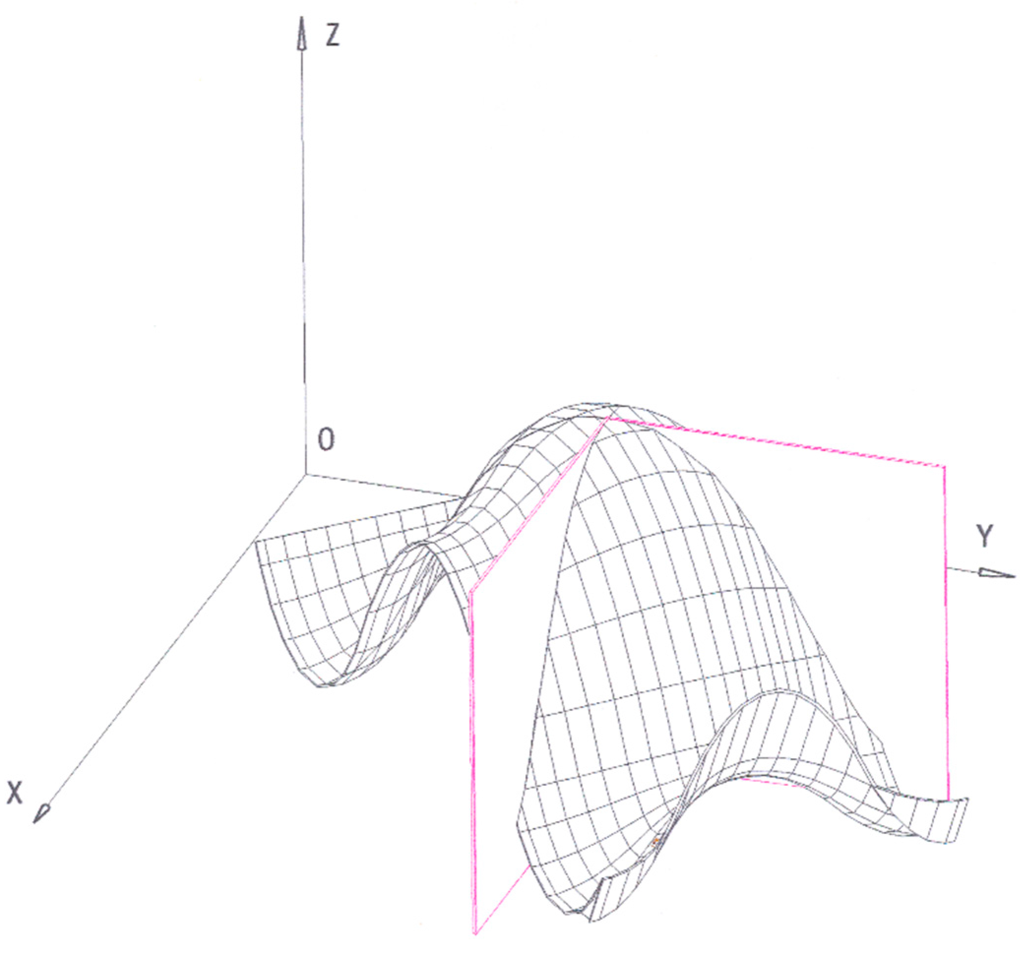
In particular, Gibbs defined a Cartesian three-fold space where the (X, Y, Z) coordinates correspond univocally to (v, η, ε) values. Within this space, the two-variables-function ε = ε (η, v)—obtained from the integration of Equation (1)—is represented by a surface that Gibbs referred to as the thermodynamic surface. Figure 1 reports a hypothetical thermodynamic surface, drawn by ourselves by means of a graphical software, according to Gibbs’ indications:

“Now the relation between the volume, entropy, and energy may be represented by a surface, most simply if the rectangular coordinates of the various points of the surface are made equal to the volume, entropy, and energy of the body in its various states. It may be interesting to examine the properties of such a surface, which we will call the thermodynamic surface of the body for which it is formed.

To fix our ideas, let the axes of v, η and ε have the directions usually given to the axes of X, Y, and Z (v increasing to the right, η forward, and ε upward).”

[7] (p. 34)

Gibbs underlines that the points lying on the surface clearly correspond to thermodynamic equilibrium states:

“When the body is not in a state of thermodynamic equilibrium, its state is not one of those, which are represented by our surface.”

[7] (p. 35)

The concept of equilibrium à la Gibbs will be clarified in a further section; here we just need to underline that the surface points are states marked by the absence of sensible motions, i.e., macroscopically static states.

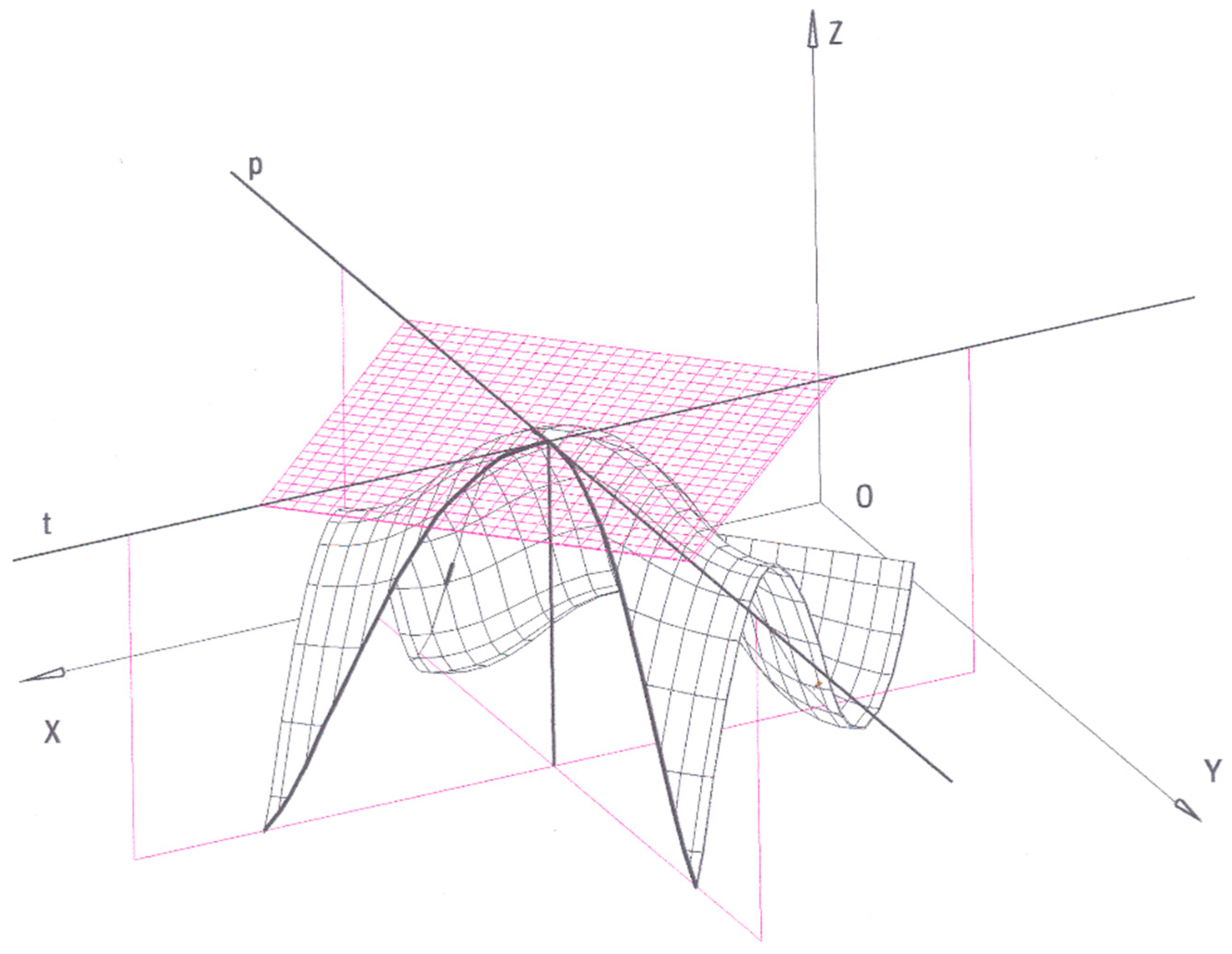
This model entails that temperature and pressure may also be geometrically represented. Maxwell—who extensively commented this point in his “Theory of Heat”—provides the following comment on temperature, whose analytical definition is given by Equation (2):

“The section of the surface by a vertical plane parallel to the meridian (i.e., the plane parallel to (Z, Y) in Figure 2) is a curve of constant volume. In this curve the temperature is represented by the rate at which the energy increases as the entropy increases, that is to say, by the tangent of the slope of the curve.”

[13] (p. 197)

In fact, it is possible to draw a plane perpendicular to the $v$ axis (i.e., characterized by $v=constant$). Its intersection with the thermodynamic surface identifies a curve that represents the dependence of energy vs. entropy at constant volume. Similarly, a plane perpendicular to the $\eta$ axis (i.e., characterized by $\eta =constant$) identifies a curve that represents the dependence of energy vs. volume at constant entropy. These two curves intersect at a specific point of the surface. An infinite number of straight lines lie on the plane tangent to the surface at that specific point (Figure 2). Amongst them, there is only one line lying on the “η = constant” plane and only one line lying on the “$v=constant$” plane. Based on Equations (2) and (3), the slope of each one of these two tangent lines correspond to t and −p, respectively. Hence, each point of the surface is associated with one and only one couple of (t, −p) values. In Gibbs’ geometrical model, these two quantities are represented as the slopes of two lines that identify the plane tangent to the surface at any point. Gibbs remarks: “Hence, the tangent plane at any point indicates the temperature and pressure of the state represented. It will be convenient to speak of a plane as representing a certain pressure and temperature, when the tangents of its inclinations to the horizon, measured as above, are equal to that pressure and temperature” [7] (p. 34).

4. Thermodynamic Equilibrium

We analyzed Gibbs’ writings with the aim of identifying where the Second Law is concealed inside Gibbs’ formal apparatus. In order to achieve this goal, we have retraced the logical path followed by Gibbs in his treatment of thermodynamic equilibrium. In the following sections we examine the steps of such logical progression, taking into account systems of increasing complexity. At first, we deal with Gibbs’ formal treatment of equilibrium in the very general case of a system that can exchange energy (but not matter) with the surroundings (for the sake of clarity, we will refer to it as closed system although this is not Gibbs’ terminology). In doing so, we make explicit a cryptic passage of Gibbs’ second paper (p. 40 of [7]) where he set forth the geometrical representation of a dissipative process leading a system towards thermodynamic equilibrium by exchanging energy with the surroundings. This formal step represents the logical point wherein the Second Law is truly embodied into Gibbs’ model. In a further step, we take under consideration the formal definition of equilibrium provided by Gibbs as regards: (i) homogeneous systems with constant chemical composition; (ii) homogeneous systems with variable chemical composition; (iii) heterogeneous systems. The comparative analysis of these three cases led us to the logical inference that their formal treatment stems from the application of appropriate boundary conditions to the results obtained for the general instance of closed systems. The final part of our analysis deals with the application of Gibbs’ formalism to a real system, made of liquid water in equilibrium with the gaseous mixture of dihydrogen, dioxygen and water.

4.1. Thermodynamic Equilibrium “à la Gibbs”

This section focuses on the pivotal concept of equilibrium, as it can be deduced from Gibbs’ writings and, especially, from his second paper [7].

A preliminary clarification is needed. Contemporary readers associate equilibrium to a condition of stability. That’s not Gibbs’ idea. Equilibrium (à la Gibbs) corresponds to a state wherein “all parts of the body are at rest” [7] (p. 39) in the sense that they are not in sensible motion [14] and this state (as it will be specified later) can be either stable or unstable. This is inferred by contrast, from passages where Gibbs refers to non-equilibrium states as dynamic states whose energetics includes necessarily a kinetic energy term:

“As the discussion is to apply to cases in which the parts of the body are in (sensible) motion, it is necessary to define the sense in which the word energy is to be used. We will use the word as including the vis viva (i.e., kinetic energy in pre–modern language) of sensible motions [15].”

[7] (p. 39)

An example of such a system is a fluid subjected to convective motions, where temperature is not uniform throughout the system and sensible motions perturb the overall mass. When temperature becomes uniform, the fluid gets to a state of rest, i.e., a macroscopically static state. This is Gibbs’ idea of equilibrium, mentioned in his second paper [7]. Hence, from the energetic standpoint, the total energy of a system not in equilibrium has to include a kinetic energy term. Potential energy and other energy contributions (e.g., due to gravitational effects) are ignored so far. Accordingly, the total energy of a fluid in motion can be written as the sum of two terms:

$$\epsilon ={\epsilon }_k+{\epsilon }_i$$

(4)

being ${\epsilon }_k$ and ${\epsilon }_i$ kinetic and internal energy, respectively.

This assumption is in line with Bridgman’s remarks that elementary thermodynamics refers to a simplified definition of energy that ignores the macroscopic energy components (e.g., kinetic, gravitational, electromagnetic…) since “elementary thermodynamics is seldom concerned with transformations involving large–scale kinetic energy. But obviously such effects are to be included” [1] (p. 57).

Whenever the system gets to a state of rest (i.e., Gibbs’ equilibrium), due to dissipative processes, macroscopic motions disappear and the kinetic energy contribution in Equation (4) is zeroed; hence the total energy reduces to internal energy. These events may be translated in geometrical terms, within the (v, η, ε) space. In fact, Gibbs points out that whenever the system is not at equilibrium “its state is not one of those, which are represented by our surface” [7] (p. 35): this means that it corresponds to a point within the (v, η, ε) space that does not belong to the thermodynamic surface. Then, the dissipative process leading the system to equilibrium is comparable to a movement along the direction of the ε axis that brings the system onto the surface. Hence, the kinetic energy term of a fluid in motion corresponds to the distance between an out-of-the-surface point and its projection on the surface along the direction of the ε axis. This means that the kinetic energy term is the discriminant between a state of sensible motion (non-equilibrium state) and a state of rest (state of equilibrium à la Gibbs, where the energy of the system is reduced to pure internal energy). In Gibbs’ elusive words, this is expressed as follows:

“If all parts of the body are at rest, the point representing its volume, entropy, and energy will be the center of gravity of a number of points upon the primitive (thermodynamic) surface. The effect of motion in the parts of the body will be to move the corresponding points parallel to the axis of ε, a distance equal in each case to the vis viva of the whole body.”

[7] (p. 39)

A crucial passage of Gibbs’ treatment is to consider how the state variables change when a system—far from equilibrium—is placed in a medium that is supposed to be at constant pressure and temperature. Gibbs’ aim was clearly to investigate “the processes which take place when equilibrium does not subsist” [7] (p. 39).

According to some authors, processes are completely disregarded by Gibbs, who would focus exclusively on the equilibrium state. This seems to be Uffink’s viewpoint: “The work of Gibbs in thermodynamics (written in the years 1873–1878) is very different from that of his European colleagues. Where Clausius, Kelvin and Planck were primarily concerned with processes, Gibbs concentrates his efforts on a description of equilibrium states” [5] (p. 52). Truesdell goes even further, stating that Gibbs turned thermodynamics into thermostatics: “Accepting the restrictions CLAUSIUS had imposed one by one in his years of retreat from irreversible processes, GIBBS eliminated processes altogether and recognized the subject in its starved and shrunken form as being no longer the theory of motion and heat interacting, no longer thermodynamics, but only thermostatics” [16] (p. 38). In fact, he remarks the absence of the temporal dimension from Gibbs’ treatment (“GIBBS proceeded to construct a strictly static theory, in which change in time played no part at all” [16] (p. 38)) and underlines its purely formal character (“true equilibrium was characterized by a genuine, mathematical maximum principle” [16] (p. 38)) enriched with the postulate that the equilibrium must be stable.

We do agree with these authors as far as the centrality of the equilibrium concept in Gibbs’ model is concerned. But we cannot agree on other issues. Clearly, thermodynamic equilibrium is a static condition (at least, at the macroscopic level), but Gibbs’ texts show very clearly that—in order to formalize its description—Gibbs had to think of an idealized dissipative process leading the system towards equilibrium. Hence, processes play a foundational role in equilibrium theory. It might be helpful recalling the Greek etymology of the word thermodynamics that derives from $\vartheta \epsilon \rho \mu \eta$(i.e., therme, heat) and $\delta \upsilon \nu \alpha \mu \iota \varsigma$(i.e., dynamis, power); hence it means heat power and not heat motion as Truesdell seems to suggest. Thus his reference to “thermostatics” sounds like a misunderstading. It must also be underlined that the requirements for equilibrium stability—which are commented at the end of this section—do emerge as a necessary consequence in Gibbs’ geometrical model and are not postulated, as Truesdell claims.

Gibbs’ description of the process leading a system towards equilibrium relies on the general case of a closed system placed inside a very large medium that is supposed to be at constant pressure and temperature. Gibbs ideally separates the system from the medium by means of a hypothetical “envelop” whose aim is to mediate the interaction between the system and the surrounding:

“…the body (is) separated from the medium by an envelop which will yield to the smallest differences of pressure between the two, but which can only yield very gradually, and which is also a very poor conductor of heat. It will be convenient and allowable for the purposes of reasoning to limit its properties to those mentioned, and to suppose that it does not occupy any space, or absorb any heat except what it transmits, i.e., to make its volume and its specific heat 0. By the intervention of such an envelop, we may suppose the action of the body upon the medium to be so retarded as not sensibly to disturb the uniformity of pressure and temperature in the latter.”

[7] (p. 39)

This ideal envelope is a conceptual artifice conceived to stress the asymmetry of the interaction between the system (body in Gibbs’ writings) and its surrounding. The surrounding is practically not affected by the system as the action of the system upon it is “so retarded as not sensibly to disturb the uniformity of pressure and temperature”. Conversely the system is affected by the energy exchange with the outside and, after a given time, it gets to the equilibrium state.

The final purpose of this ideal experiment is to find the relationships between the variables that describe the initial and final state of the system:

“Now let us suppose that the body having the initial volume, entropy, and energy, $v^{\prime }, {\eta }^{\prime } \text{and} {\epsilon }^{\prime }$ is placed (…) in a medium having the constant pressure P and temperature T, and by the action of the medium and the interaction of its own parts comes to a final state of rest in which its volume, etc., are $v^{″}, {\eta }^{″} \text{and} {\epsilon }^{″}$; we wish to find a relation between these quantities.”

[7] (p. 40)

In the following subsections we discuss how energy, entropy and volume change under the effect of such an idealized process.

4.2. Energy Variation in a Dissipative Process

Assuming that the medium’s size is such that heating or compressing it “within moderate limits will have no appreciable effect upon its pressure and temperature” the fundamental equation for the medium can be written as:

$$dE=TdH-PdV$$

(5)

being E, H and V energy, entropy [17] and volume (Gibbs used capital Greek letters to refer to the medium and minuscule Greek letters to refer to the system).

If pressure (P) and temperature (T) are constant throughout the process, the integration of Equation (5) between an initial state (with energy E′) and a final state (with energy E′′) brings to:

$$E^{″}- E^{\prime }=T{H}^{″}-T{H}^{\prime }-P{V}^{″}+P{V}^{\prime }$$

(6)

But the presence of the envelope allows neglecting any effect of the system on the surroundings; hence Equation (6) is independent from the process leading the system towards equilibrium. Based on Gibbs’ hypothesis, the total energy of the medium is not affected and so:

$$E^{″}=E^{\prime }$$

(7)

Turning our attention to the system, the problem is to establish how energy, entropy and volume vary as the result of the dissipative process that leads the system towards equilibrium and zeroes kinetic energy. The envelope allows the system to exchange energy with its surroundings. Hence, based on the energy conservation principle, two possibilities can be foreseen:

• Kinetic energy is dissipated inside the system itself; hence internal energy increases accordingly. In such case, the total energy of the system does not change since the internal energy gain compensates the kinetic energy loss. Being ${\epsilon }_k^{\prime }$ the kinetic energy of non-equilibrium initial state and ${\epsilon }_i^{\prime \prime }\text{ and }{\epsilon }_i^{\prime }$ the internal energies in the final and initial states, respectively, the previous energy balance translates as:

  $${\epsilon }_i^{\prime \prime }={\epsilon }_i^{\prime }+{\epsilon }_k^{\prime }$$

  (8)
  Hence, from Equation (4):

  $${\epsilon }^{″}={\epsilon }^{\prime }$$

  (9)
• Kinetic energy is dissipated outside the system (i.e., towards the medium through the envelope). Hence the total energy of the system decreases and the following inequality holds valid:

  $${\epsilon }^{″}<{\epsilon }^{\prime }.$$

  (10)

In summary, when a system—far from equilibrium—is placed in a medium at constant temperature and pressure, wrapped by the ideal Gibbs’ envelope, its total energy changes according to the following inequality:

$${\epsilon }^{″}\le {\epsilon }^{\prime }.$$

(11)

The sign of equality holds only if kinetic energy is completely transformed into internal energy.

As far as we consider “the body and the surrounding” together, the total energy must be the sum of the energies of each component. Hence, the inequality resulting from the sum of expressions (7) and (11) holds true:

$$E^{″}+{\epsilon }^{″}\le E^{\prime }+{\epsilon }^{\prime },$$

(12)

or in Gibbs’ own words:

“As the sum of the energies of the body and the surrounding medium may become less, but cannot become greater (this arises from the nature of the envelope supposed), we have $E^{″}+ {\epsilon }^{″}\le E^{\prime }+ {\epsilon }^{\prime }.$”

[7] (p. 40)

As “the body and the surroundings” constitute an isolated system, Equation (12) might imply a formal violation of the energy conservation principle. Nevertheless, it must be borne in mind that the incoherence is purely formal as it stems from the features that Gibbs assigns to the envelope. In fact—by construction—it prevents the transmission of the body’s kinetic energy to the medium without forbidding the medium’s action over the body. Despite the apparent oddity of the envelope’s property, the conclusion is consistent with the pragmatic, engineeristic assumption that the difference in size between the medium and the system justifies ignoring the contribution of the system to the energy of the medium, whereas the contrary is not true. In other words, the energy amount that is actually disregarded is quantitatively negligible as compared to the internal energy component. Likewise, in current engineering thermodynamics, the kinetic and potential energy for either the system or any flowing streams are ignored when their contributions are negligible as compared to the other energy components.

4.3. Entropy Variation in a Dissipative Process

As far as entropy is concerned, Gibbs’ reasoning can be made explicit by considering that the sum of “the body and the surrounding”—taken as a unique whole—corresponds to Clausius’ concept of universe (i.e., an adiabatically isolated system in current language). In this instance Clausius’ Second Law translates into:

$$dS\ge 0;$$

(13)

Hence, the entropy of “the body and the surrounding” cannot decrease. In Gibbs’ notation this condition can be written as:

$$H^{″}+ {\eta }^{″}\ge H^{\prime }+ {\eta }^{\prime }.$$

(14)

As regards expression (14), Gibbs simply remarks that “the sum of the entropies may increase but cannot diminish” [7] (p. 40). In line with his hermetic style, Gibbs does not detail this logical step. It remains that expression (14) represents a pivotal point inside all Gibbs’ formal apparatus since this logical step marks the truly conceptual entrance of Clausius’ Second Law inside Gibbs’ equilibrium theory.

4.4. Volume Invariance

As far as volume is concerned, Gibbs noted [7] (p. 40):

“Lastly, it is evident that:

$$V^{″}+ v^{″}=V^{\prime }+ v^{\prime }.”$$

(15)

Again, the assumption is based on the identification of “the body and the surrounding” with an isolated system, whose volume is supposed invariant with respect to any thermodynamic transformation.

4.5. Getting to a “Geometrical” Synthesis

Finally, Gibbs provides a formal synthesis of the aforementioned idealized process leading a system to equilibrium. More precisely he builds up a linear combination of Equations (6), (12), (14) and (15), according to the following modus operandi:

• Equation (6) is arranged to give:

  $$-E^{″}+T{H}^{″}-P{V}^{″}= -E^{\prime }+T{H}^{\prime }-P{V}^{\prime };$$

  (16)
• Equation (12) is used as it is:

  $$E^{″}+ {\epsilon }^{″}\le E^{\prime }+ \epsilon \prime ;$$
• both members of Equation (14) are multiplied by $–T$

  $$-T{H}^{″}-T {\eta }^{″} \le -T{H}^{\prime }-T {\eta }^{\prime };$$

  (17)
• both members of Equation (15) are multiplied by $P$

  $$P{V}^{″}+ P{v}^{″}=P{V}^{\prime }+ P{v}^{\prime },$$

  (18)

The sum of these four equations gives rise to the following inequality:

$${\epsilon }^{″}-T{\eta }^{″}+ {Pv}^{″}\le {\epsilon }^{\prime }-T{\eta }^{\prime }+ {Pv}^{\prime }.$$

(19)

that has a precise geometrical correspondence in Gibbs’ representation of the thermodynamic space, shown in Figure 3.

Gibbs comments this geometrical description as follows:

“Now the two members of this equation (i.e.,Equation (19)) evidently denote the vertical distances of the points $\left(v^{″},{\eta }^{″}, {\epsilon }^{″}\right)$ and $\left(v^{\prime },{\eta }^{\prime }, {\epsilon }^{\prime }\right)$ above the plane passing through the origin and representing the pressure P and temperature T. And the equation expresses that the ultimate distance is less or at most equal to the initial. It is evidently immaterial whether the distances be measured vertically or normally, or that the fixed plane representing P and T should pass through the origin; but distances must be considered negative when measured from a point below the plane.”

[7] (p. 40)

In summary, a system far from equilibrium—surrounded by a medium at constant temperature and pressure—moves towards equilibrium through a process that “will ensue that the distance of the point representing the volume, entropy, and energy of the body from that fixed plane (i.e., the (T, P) plane) will be diminished” [7] (p. 41).

4.6. Stability Criteria

The relevance of this geometrical representation of the dissipative process is not limited to its formal elegance. In fact, the geometrical translation of thermodynamics principles carried out by Gibbs has a clear epistemic role: it is a formal structure through which Gibbs justifies the equilibrium stability. Within this geometrical frame of ideas, Gibbs conceives three distinct possibilities, that he calls stable, unstable and neutral equilibrium, respectively, and put them in relation with “the geometrical properties of the [thermodynamic] surface” [7] (p. 39):

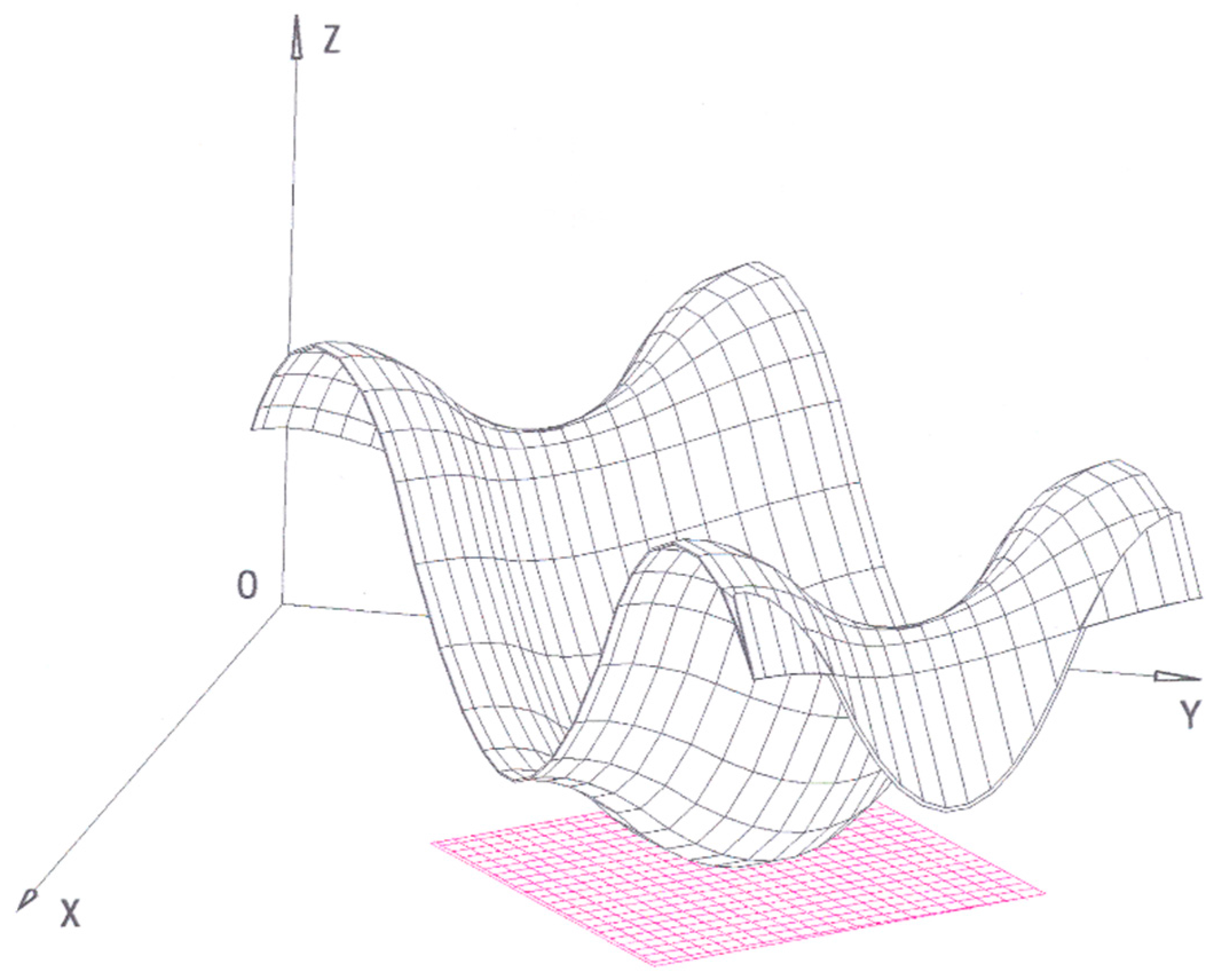
(1)

The thermodynamic surface is all above the tangent plane (Figure 4). In this case the point common to the surface and the plane corresponds to a stable state. In Gibbs’ own words:

“Now, if the form of the surface be such that it falls above the tangent plane except at the single point of contact, the equilibrium is necessarily stable.”

[7] (p. 42)

To justify this statement, Gibbs refers to Equation (19) and its geometrical meaning. More precisely, he sustains that if a stable equilibrium state is somehow altered, the system spontaneously tries to go back to its initial position. According to Equation (19), the geometrical effect of this process is to lead the system to a point that is closer to the (T, P) plane as compared to the perturbed system:

“… for if the condition of the body be slightly altered, either by imparting sensible motion to any part of the body, or by slightly changing the state of any part, or by bringing any small part into any other thermodynamic state whatever, or in all of these ways, the point representing the volume, entropy, and energy of the whole body will then occupy a position above the original tangent plane, and the proposition above enunciated (Equation (19)) shows that processes will ensue which will diminish the distance of this point from that plane, and that such processes cannot cease until the body is brought back into its original condition, when they will necessarily cease on account of the form supposed of the surface.”

[7] (p. 42)

(2)

If the surface is all underneath the tangent plane, the common point to the surface and the plane corresponds to an unstable state.

“On the other hand, if the surface have such a form that any part of it falls below the fixed tangent plane, the equilibrium will be unstable. For it will evidently be possible by a slight change in the original condition of the body (that of equilibrium with the surrounding medium and represented by the point or points of contact) to bring the point representing the volume, entropy, and energy of the body into a position below the fixed tangent plane, in which case we see by the above proposition that processes will occur which will carry the point still farther from the plane, and that such processes cannot cease until all the body has passed into some state entirely different from its original state.”

[7] (p. 42)

According to Gibbs’ model, a system in an unstable equilibrium state can only evolve towards a stable one. In fact, any movement of such system along the thermodynamic surface causes the system itself to move away from the initial point, thus bringing it further below the tangent plane. In a sense, the system glides on the surface until it finds stable equilibrium conditions. Even without reference to Gibbs’ definition, Planck found a clear example of unstable equilibrium (i.e., labilen Gleichgewicht) in the case of the explosion of a gaseous mixture. In such a case, increasing energy of “a convenient but arbitrary small amount” could trigger off sudden and dramatic transformations:

“Von diesem Gesichtspunkt aus betrachtet, befindet sich z. B. ein Knallgasgemenge nur im labilen Gleichgewicht, weil die Hinzufügung einer geeigneten, aber beliebig kleinen Menge Energie (z. B. eines elektrischen Funkens, dessen Energie im Vergleich zu der des Gemenges verschwindend klein sein kann) eine endliche Zustandsänderung, also einen Uebergang zu einem Zustand grösserer Entropie, zur Folge hat.”

[18] (p. 474)

(3)

The third circumstance occurs when the surface does not “anywhere fall below the fixed tangent plane, nevertheless meets the plane in more than one point”. Gibbs names this instance neutral equilibrium [7] (p. 42) due to its intermediate character between the cases already considered. He further specifies this definition by remarking “if any part of the body be changed from its original state into that represented by another point in the thermodynamic surface lying in the same tangent plane, equilibrium will still subsist” [7] (p. 42).

In other words, neutral equilibrium subsists when the same fixed (T, P) plane has more than one point of tangency with respect to the thermodynamic surface. These tangency points correspond to thermodynamic states that can coexist in equilibrium. The physical meaning of this formal circumstance can be interpreted by considering what happens at the triple point of a pure substance. This point corresponds by definition to a unique couple of (T, P) values. Then, in Gibbs’ geometrical model a triple point can be associated to a fixed plane whose slope is given by that very same couple of (T, P) values. By definition, three phases coexist in equilibrium at a triple point. In Gibbs’ geometrical representation, these three phases correspond to three points of the thermodynamic surface “lying in the same tangent plane”.

To this regard, Cerciniani remarks that the concept of neutral equilibrium “answered the question that had puzzled Maxwell when, in July 1871, he was working on Andrews’ result on the continuity of the liquid and gaseous states” [4] (p. 137). Maxwell’s question was: “in physical terms, what is the condition determining the pressure at which gas and liquid can coexist in equilibrium?” He argued that the difference in internal energy between the two phases must be a minimum at the pressure where they coesist. Nevertheless, “he would change his mind after reading Gibbs’ paper” [4] (p. 137).

5. Dealing with Isolated Systems

In the previous section we have retraced the meaning of Gibbs’ equilibrium and have reconstructed its formal representation in the general case of systems that can exchange energy with the surroundings, whereas matter exchange is never mentioned. The present section deals with different kinds of isolated systems, chosen by Gibbs as cases of great interest.

Before entering into the merits of Gibbs’ description, it seems worth reminding that a definition of isolated systems is not straightforward as the adjective “isolated” has several philosophical implications that are matter of discussion. Once again, we report Bridgeman’s remark:

“The business of ‘isolating’ a system perhaps requires more discussion. What shall we say to one who claims that no system can ever be truly ‘isolated’, for he may maintain that the velocity of electromagnetic disturbances within it or the value of the gravitational constant of the attractive force between its parts is determined by all the rest of the matter in the universe? To this all that can be answered is that this is not the sort of thing contemplated; even if an observer stationed on the surface enclosing the system is able to see other objects outside the surface and at a distance from it, the system may nevertheless still be pronounced isolated. It would probably be impossible under these conditions to give a comprehensive definition of what is meant in thermodynamics by ‘isolation’, but the meaning would have to be conveyed by an exhaustive cataloguing of all the sorts of things which might conceivably occur to an observer stationed on the enclosing surface, with an explicit statement that this or that sort of thing does or does not mean isolation.”

[1] (p. 81)

A philosophical discussion on this matter is out of this paper’s aim. We do limit our analysis to the specification of what is meant by isolation in Gibbs’ thermodynamics. Gibbsian isolated system—in addition to being impermeable to any mass exchange—is to be understood as adiabatically and mechanically isolated, in the sense that it does not exchange either heat or work with the outside. Hence, isolation implies also an isochoric condition that physically corresponds to volume invariance.

Amongst isolated systems, Gibbs further distinguishes between homogeneous and heterogeneous systems. Homogeneous systems are described as follows:

“By homogeneous is meant that the part in question is uniform throughout, not only in chemical composition, but also in physical state.”

[8] (p. 63)

In addition, it must be clear that—amongst homogeneous systems—Gibbs considers as chemically homogeneous a system whose composition is uniform throughout any of its part, despite the fact that it contains one or more chemical components (e.g., a solution is made of at least two components but it is homogeneous in the sense that its chemical composition is uniform throughout the system). Gibbs also makes clear that a homogeneous system must be physically uniform, i.e., it must consist of one single phase.

At first, he considers the case where “the amount and kind of matter in this homogeneous mass (can be considered) as fixed”. In these conditions, the total energy is only function of entropy and volume and the differentials of these quantities satisfy the following relation:

$$d\epsilon =td\eta -pdv.$$

(20)

Then Gibbs considers a more complex case, described as follows:

“If we consider the matter in the mass [i.e., system] as variable, and write $m_1, m_2\dots m_n$ for the quantities of the various substances $S_1, S_2\dots S_n$ of which the mass is composed, ε will evidently be a function of $\eta , v, m_1, m_2\dots m_n$ and we shall have for the complete value of the differential of ε:

$$d\epsilon =td\eta -pdv+{\mu }_{1}d{m}_1+{\mu }_{2}d{m}_2\dots {\mu }_{n}d{m}_n$$

(21)

${\mu }_1, {\mu }_2\dots {\mu }_n$ denoting the differential coefficients of ε taken with respect to $m_1, m_2\dots m_n$.” [8] (p. 63).

Unfortunately Gibbs does not provide a clear-cut definition of heterogeneous system: it has to be logically deduced, by contrast, from the above reported definitions as well as from the use of the adjective “heterogeneous” found in Gibbs’ writings. For this reason Le Chatelier—in his French translation of Gibbs’ works—found necessary to clarify such meaning and to justify his choice of translation:

“Le mot hétérogène a été traduit par chimique parce qu'en français le mot hétérogène sert habituellement indiquer une différence d'état physique tandis qu’il exprime ici une différence d’état chimique.”

[2] (p. 1)

Le Chatelier expresses the idea that the features of heterogeneous systems are opposite to those that Gibbs assigns to homogeneous systems. Hence, a heterogeneous system is uniform neither in physical state nor in chemical composition (e.g., a system made by two separated phases with different chemical composition).

In the following section we report and analyse how equilibrium conditions expressed by Equation (19) were adapted for handling chemical systems. Gibbs approached this challenge by considering cases of increasing complexity, starting from the idealized circumstance of mechanically isolated systems with fixed “amount and kind of matter” up to systems with variable chemical composition. We also highlight and discuss how the Second Law is disguised in the treatment of these increasingly complex material systems.

6. Gibbs’ principle Applied to Homogeneous Systems

Let’s take the case of homogeneous isolated systems with constant chemical composition for which Gibbs formulates (without providing any demonstration) the “necessary and sufficient” conditions of equilibrium through the famous principle of maximal entropy and minimal energy:

“The criterion of equilibrium for a material system, which is isolated from all external influences, may be expressed in either of the following entirely equivalent forms:

• For the equilibrium of any isolated system it is necessary and sufficient that in all possible variations of the state of the system, which do not alter its energy, the variation of its entropy shall either vanish or be negative. If ε denote the energy, and η the entropy of the system, and we use a subscript letter after a variation to indicate a quantity of which the value is not to be varied, the condition of equilibrium may be written:

  $${(\delta \eta )}^{ }{}_{\epsilon }\le 0,$$

  (22)
• For the equilibrium of any isolated system it is necessary and sufficient that in all possible variations in the state of the system, which do not alter its entropy, the variation of its energy shall either vanish or be positive. This condition may be written:

  (δε)_η ≥ 0”.  [8] (p. 56)

  (23)

According to Gibbs, the equilibrium state of an isolated system, undergoing a change at constant energy, corresponds to the “maximum entropy” state. Vice versa, at constant entropy conditions, the equilibrium is achieved when minimum energy is attained.

Gibbs’ aforementioned statement does not specify if the equilibrium state is stable or unstable. Stability conditions are specified in a subsequent passage, wherein they are related to “the absolute value of the variations”:

“But to distinguish the different kinds of equilibrium in respect to stability, we must have regard to the absolute values of the variations. We will use ∆ as the sign of variation in those equations, which are to be construed strictly, i.e., in which infinitesimals of the higher orders are not to be neglected.

With this understanding, we may express the necessary and sufficient conditions of the different kinds of equilibrium as follows; for stable equilibrium:

$${\left(\Delta \eta \right)}_{\epsilon }<0, i.e., {\left(\Delta \epsilon \right)}_{\eta }>0;$$

(24)

(…)

and for unstable equilibrium there must be some variations for which:

$${\left(\Delta \eta \right)}_{\epsilon }>0$$

(25)

i.e., there must be some for which:

$${\left(\Delta \epsilon \right)}_{\eta }<0$$

(26)

while in general:

(δη)_ε ≤ 0, i.e., (δε)_η ≥ 0 ”.  [8] (p. 57)

(27)

In other words a stable equilibrium state corresponds to an absolute extremal point of entropy (maximum) or energy (minimum). Max Planck provides an interpretation of equilibrium stability, with special attention to the principle of maximal entropy, remarking that the “stable state of equilibrium” corresponds to “the absolute maximum” of entropy [19].

It is surprising to realize that, although Gibbs’ principle is justified from the cognitive standpoint—and many authors such as Maxwell, van der Waals, Kohnstamm, Callen and Buchdahl have endorsed his approach [5] (p. 53)—its formal justification is lacking. As a matter of fact, in Gibbs’ writings there is not explicit demonstration of these principles. Uffink highlights the character of inference of Gibbs treatment, underlying—at the same time—its strict relationship with Clausius’ Second Law:

“Actually, Gibbs did not claim that this statement presents a formulation of the second law. But, intuitively speaking, the Gibbs principle, often referred to as principle of maximal entropy, does suggest a strong association with the second law. Gibbs corroborates this suggestion by placing Clausius’ famous words (‘Die Entropie der Welt strebt ein Maximum zu’) as a slogan above his article. Indeed, many later authors do regard the Gibbs principle as a formulation of the second law.

Gibbs claims that his principle can be seen as ‘an inference naturally suggested by the general increase of entropy which accompanies the changes occurring in any isolated material system’. He gives a rather obscure argument for this inference.”

[5] (p. 52)

In the following lines we show as, starting from the mathematical representation of the dissipative process leading a system to equilibrium as given by Equation (19), it is possible to outline a formal justification of Gibbs’ principle and to highlight a logical pathway consistent with Gibbs’ conclusions.

Equation (19) can be synthetically written as follows:

$$\delta {\epsilon }^{ }-T\delta {\eta }^{ }+ P\delta v\le 0,$$

(28)

where $\delta {\epsilon }^{ }$, $\delta {\eta }^{ }$and $\delta v$ represent finite variations of energy, entropy and volume respectively [20]. Consistently with Gibbs’ reasoning that delivered Equation (19), Equation (28) is a mathematical representation of how energy, entropy and volume can vary during an arbitrary process that leads a homogeneous system from a state wherein “equilibrium does not subsist” towards an equilibrium state. Conversely, if we assume that a system is at equilibrium and by means of whatever process we alter its state in order to push it towards non-equilibrium, then the energy, entropy and volume variations will satisfy the inequality opposite to Equation (28):

$$\delta {\epsilon }^{ }-T\delta {\eta }^{ }+ P\delta v\ge 0.$$

(29)

Let’s apply Equation (29) in the following two conditions:

(1)

The system does not change its volume (i.e., it is mechanically isolated) and the transformation does not alter energy value. These two constraints mathematically correspond to $\delta v=0$ and $\delta \epsilon =0$, implying that Equation (29) transforms into:

$$\delta {\eta }^{ }\le 0.$$

(30)

This means that, by altering the equilibrium state of a system through a process wherein energy and volume are kept constant, entropy can either decrease or—at least—remain equal. In other words, the equilibrium state of a system, maintained at constant energy and volume, corresponds to a maximum of entropy; that’s nothing but the principle of maximal entropy, or the first clause of Gibbs’ principle.

(2)

The system does not change its volume (i.e., it is mechanically isolated) and the transformation does not alter entropy value. These two constraints mathematically correspond to $\delta v=0$ and $\delta \eta =0$ implying that Equation (29) transforms into:

$$\delta {\epsilon }^{ }\ge 0.$$

(31)

This means that, by altering the equilibrium state of a system through a process wherein entropy and volume are kept constant, energy can either increase or—at least—remain equal. It is self-evident to recognize here the principle of minimal energy, corresponding to the second clause of Gibbs’ principle.

7. Towards Chemical Equilibrium

In the present section we retrace how Gibbs’ principle was extended to systems with variable chemical composition. The analysis of his text shows that this huge epistemic operation was based on the assumption that the principle of minimal energy (and maximal entropy) holds true for homogeneous isolated systems with variable chemical composition. This undemonstrated assumption opened the way to the treatment of what he calls “heterogeneous masses”, i.e., systems “divided into parts so that each part is homogeneous, and consider such variations in the energy of the system as are due to variations in the composition and state of the several parts remaining (at least approximately) homogeneous, and together occupying the whole space within the envelop” [8] (p. 64). The reference to “variations in the composition and state of the several parts” implies that these subsystems are subjected to chemical transformations that may result also in substances, not formerly present in a particular subsystem—provided that these substances, or their components, are to be found in some part of the whole given mass. In Gibbs own words:

“The substances $S_1, S_2\dots S_n$, of which we consider the mass composed, must of course be such that the values of the differentials shall be independent, and $d{m}_1, d{m}_2\dots d{m}_n$ shall express every possible variation in the composition of the homogeneous mass considered, including those produced by the absorption of substances different from any initially present. It may therefore be necessary to have terms in the equation relating to component substances which do not initially occur in the homogeneous mass considered, provided, of course, that these substances, or their components, are to be found in some part of the whole given mass.”

[8] (p. 63)

As regards the heterogeneous system, the amounts of its elementary chemical components (the components in Gibbs’ text) are constant, although the distribution and combination of such components may vary within the single homogeneous subsystems.

In summary, the heterogeneous system is modeled as a set of homogeneous subsystems—mutually in contact—wrapped by “a rigid and fixed envelop, which is impermeable to and unalterable by any of the substances enclosed, and perfectly non–conducting to heat” [8] (p. 62).

Gibbs specifies “that the supposition of [this] rigid and non-conducting envelop enclosing the mass under discussion involves no real loss of generality” since “if any mass of matter is in equilibrium, it would also be so, if the whole or any part of it were enclosed in an envelop as supposed”. He concludes:

“the conditions of equilibrium for a mass thus enclosed are the general conditions which must always be satisfied in case of equilibrium.”

[8] (p. 62)

It follows that equilibrium conditions within each subsystem can be treated by referring to the same conditions already formulated for isolated systems—as formalized by Equations (22) and (23). The whole heterogeneous system will find its equilibrium state if the sum of equilibrium conditions in each single subsystem holds: the sum of energy variations of each subsystem ($\delta {ϵ}^{\prime }+\delta {\epsilon }^{″}+\dots$) has to be positive or null. Based on this premises, Gibbs explicitly elaborated the following equilibrium condition:

$$\delta {ϵ}^{\prime }+\delta {\epsilon }^{″}+\dots \ge 0$$

(32)

by taking into account the constraints characterizing the heterogeneous system—according to how it was modeled. This means that the system is isolated, either mechanically or chemically, and undergoes changes at constant entropy. Hence, thermodynamic processes—including chemical reactions—taking place within the system will be isoentropic, isochoric and without any changes of total quantities of any component substance. These constraints are mathematically expressed by the following equations that we recall from Gibbs’ original paper:

$$\delta {\eta }^{\prime }+ \delta {\eta }^{″}+ \delta {\eta }^{‴}+\dots =0$$

(33)

$$\delta v^{\prime }+ \delta v^{″}+ \delta v^{‴}+\dots =0$$

(34)

$$\delta m_1{}^{\prime }+ \delta m_1{}^{″}+ \delta m_1{}^{‴}+\dots =0$$

(35)

$$\delta m_2{}^{\prime }+ \delta m_2{}^{″}+ \delta m_2{}^{‴}+\dots =0$$

(36)

…

$$\delta m_n{}^{\prime }+ \delta m_n{}^{″}+ \delta m_n{}^{‴}+\dots =0.$$

(37)

By replacing the energy definition expressed by Equation (21) into Equation (32), Gibbs attains the following expression of the equilibrium condition:

$$\begin{gathered} t^{\prime }d{\eta }^{\prime }-p^{\prime }d{v}^{\prime }+{{\mu }^{\prime }}_{1}d{m^{\prime }}_1+{{\mu }^{\prime }}_{2}d{m^{\prime }}_2\dots {{\mu }^{\prime }}_{n}d{m^{\prime }}_n \\ +t^{″}d{\eta }^{″}-p^{″}d{v}^{″}+{{\mu }^{″}}_{1}d{m^{″}}_1+{{\mu }^{″}}_{2}d{m^{″}}_2\dots {{\mu }^{″}}_{n}d{m^{″}}_n+\dots \ge 0 \end{gathered}$$

(38)

For the sake of clarity, superscripts of expression (38) refer to each subsystem, whereas subscript refers to each substance. This equation deserves some comments. Under the constraints expressed by Equations (33)–(37) it can be deduced that Equation (38) holds if and only if t and p have the same values throughout the entire heterogeneous system and if and only if the coefficients μ—relative to the various substances—have the same values in all the subsystems. These conditions are summarized in

Table 2. Summary of the three equilibrium conditions for heterogeneous systems.

Type of Equilibrium	Equilibrium Conditions	Equation Number
Thermal	$t^{\prime }=t^{″}=t^{‴}=\dots$	(39)
Mechanical	$p^{\prime }=p^{″}=p^{‴}=\dots$	(40)
Chemical	${{\mu }^{\prime }}_1={{\mu }^{″}}_1={{\mu }^{‴}}_1=\dots$	(41)
	${{\mu }^{\prime }}_2={{\mu }^{″}}_2={{\mu }^{‴}}_2=\dots$
	${{\mu }^{\prime }}_3={{\mu }^{″}}_3={{\mu }^{‴}}_3=\dots$

.

This reformulation of equilibrium conditions leads to a relevant novelty given by the role of differential coefficients μ, for which Gibbs provides a name and a physical meaning:

“If we call a quantity μ_x, as defined by such an Equation as (21) (numberings according to the present paper), the potential for the substance S_x in the homogeneous mass considered, these conditions (i.e., chemical equilibrium conditions) may be expressed as follows:

The potential for each component substance must be constant throughout the whole mass.”

[8] (p. 65)

In other words, Gibbs exploits potentials as a formal tool for defining chemical equilibrium on a formal basis. In fact, chemical equilibrium is attained when the potential of each substance becomes uniform throughout the heterogeneous system.

This epistemic approach allowed Gibbs to obtain a formal apparatus, wherein the above equations—in their whole—represent a general definition of thermodynamic equilibrium in a heterogeneous system accounting for thermal, mechanical and chemical phenomenology. Gibbs defines this composite nature of equilibrium as follows:

“Equations (39) and (40) [numberings according to the present paper] express the conditions of thermal and mechanical equilibrium, viz., that the temperature and the pressure must be constant throughout the whole mass. In Equation (41) we have the conditions characteristic of chemical equilibrium.”

[8] (p. 65)

For the sake of clarity, we would like to apply this treatment to the specific case—mentioned by Gibbs in his text—of “equilibrium in a vessel containing water and free hydrogen and oxygen.”

[8] (p. 63)

Gibbs specifies that this heterogeneous system consists in two homogeneous subsystems, of which one is gaseous and includes three components, while the second is liquid. We represent it in the following expression (42) and use the symbol ⇄ for designating the equilibrium:

$${\left(H_2+O_2+H_{2}O\right)}_g\rightleftarrows {\left(H_{2}O\right)}_l$$

(42)

According to Equation (21), the differential expression of energy for the homogeneous gaseous subsystem may be formalized as follows:

$$d\epsilon =td\eta -pdv+{\mu }_{H_2}d{m}_{H_2}+{\mu }_{O_2}d{m}_{O_2}+{\mu }_{{\left(H_{2}O\right)}_g}d{m}_{{\left(H_{2}O\right)}_g}$$

(43)

As far as the liquid subsystem is concerned, the differential form of energy is likely given by:

$$d\epsilon ={\left(td\eta \right)}_l-{\left(pdv\right)}_l+{\mu }_{{\left(H_{2}O\right)}_l}d{m}_{{\left(H_{2}O\right)}_l}$$

(44)

The heterogeneous system in its whole can find its equilibrium state, if the three equations reported in Table 2 are satisfied. In the specific case of this example they translates as follows:

$$t_l=t_g; p_l=p_g; {\mu }_{{\left(H_{2}O\right)}_l}={\mu }_{{\left(H_{2}O\right)}_g}$$

(45)

Starting from this conceptual structure Gibbs provides a further enrichment of his thermodynamic model by introducing new functions and fundamental equations. The meaning of the adjective fundamental is clarified in the following passage, where Gibbs comments Equation (21) that relates all state variables:

“This will make n + 3 independent known relations between the n + 5 variables, $\epsilon , \eta , v, m_{1 }, m_2, \dots , m_n, t, p, {\mu }_{1 }, {\mu }_2,\dots , {\mu }_{n }$. These are all that exist, for of these variables, n + 2 are evidently independent. Now upon these relations depend a very large class of the properties of the compound considered, we may say in general, all its thermal, mechanical, and chemical properties, so far as active tendencies are concerned, in cases in which the form of the mass does not require consideration. A single equation from which all these relations may be deduced we will call a fundamental equation for the substance in question.”

[8] (p. 86)

Actually Gibbs did not originally conceive the idea of condensing all properties of a fluid in a single mathematical expression. He bestows to Massieu the idea of characteristic functions of a fluid and defined the following thermodynamic quantities:

$$\psi =\epsilon -t\eta$$

(46)

and:

$$\zeta =\epsilon -t\eta +pv$$

(47)

The corresponding fundamental equations are derived by differentiation and comparison with Equation (21):

$$d\psi =-\eta dt-pdv+{\mu }_{1}d{m}_1+\dots {\mu }_{n}d{m}_n$$

(48)

$$d\zeta =-\eta dt+vdp+{\mu }_{1}d{m}_1+\dots {\mu }_{n}d{m}_n.$$

(49)

In current thermodynamics, functions $\psi$ and $\zeta$ are Helmholtz’s and Gibbs’ functions, respectively (

Table 3. Correspondence between the types used in Gibbs’ writings and the current thermodynamic notation.

Gibbs’ Greek Scripts	Original Gibbs’ Definition	Current Symbols	Current Definition	Current Variable Name
$\chi$	$\chi =\epsilon +pv$	$H$	$H=U+pV$	Enthalpy
$\psi$	$\psi =\epsilon -t\eta$	$A$	$A=U-TS$	Helmholtz’s function
$\zeta$	$\zeta =\epsilon -t\eta +pv$ or $\zeta =\chi -t\eta$	$G$	$G=H-TS$	Gibbs’ function

).

A third function is defined within the same logical framework:

$$\chi =\epsilon +pv$$

(50)

that in current thermodynamics corresponds to enthalpy.

Within this formal structure, energy $\epsilon$ plays the role of primitive fundamental function since $\psi$, $\zeta$ and $\chi$ can be derived from it through Legendre transformations; hence, they contain exactly the same information as Equation (1).

Within specific boundary conditions, these functions assume distinctive physical meaning that allowed Gibbs to formulate new equilibrium conditions, summarised in

Table 4. Summary of Gibbs’ fundamental equations and conditions of equilibrium, quoted from Gibbs’ third paper [8] (p. 87–88).

Thermodynamic Variables	Fundamental Equations	Equilibrium Conditions
$\epsilon , \eta , v, m_{1, } m_2, \dots , m_n$	$d\epsilon =+td\eta -pdv+{\mu }_{1}d{m}_1+\dots {\mu }_{n}d{m}_n$	${\left(\delta \epsilon \right)}_{\eta }\ge 0$ or ${\left(\delta \eta \right)}_{\epsilon }\le 0$
$\chi , \eta , p, m_{1, } m_2, \dots , m_n$	$d\chi =+td\eta +vdp+{\mu }_{1}d{m}_1+\dots {\mu }_{n}d{m}_n$
$\psi , t, v, m_{1, } m_2, \dots , m_n$	$d\psi =-\eta dt-pdv+{\mu }_{1}d{m}_1+\dots {\mu }_{n}d{m}_n$	${\left(\delta \psi \right)}_t\ge 0$
$\zeta , t, p, m_{1, } m_2, \dots , m_n$	$d\zeta =-\eta dt+vdp+{\mu }_{1}d{m}_1+\dots {\mu }_{n}d{m}_n$	${\left(\delta \zeta \right)}_{p,t}\ge 0$

together with the fundamental equations. This matter is widely discussed in the literature and we would like to mention Bordoni that—in this regard—remarks:

“The function ψ represented ‘the force function of the system for constant temperature’, in brief the mechanical work done, ‘just as -ε is the force function for constant entropy’. In transformations with equal temperature in the initial and final states, the function ψ played the role of the internal energy ε, and the condition of equilibrium became:

$${\left(\delta \psi \right)}_t\ge 0$$

(51)

Gibbs showed that the function $\zeta$ played a similar role in transformations maintaining equal temperature and pressure in their initial and final states, so that:

$${\left(\delta \zeta \right)}_{t,p}\ge 0$$

(52)

Also the function χ could assume a specific meaning under specific conditions: when ‘the pressure is not varied’:

$$d\chi =d\epsilon +pdv=dQ-dW+pdv=dQ$$

(53)

In other words, the function χ could be qualified as ‘the heat function for constant pressure’, and its decrease represents ‘the heat given out by the system’ [21] (p. 47).

As the final step of our analysis, we would like to comment the application of a particular equilibrium condition—given in terms of $\zeta$ function—to a gaseous mixture made by free dihydrogen and dioxygen and water vapour. This example corresponds to a homogeneous system with variable chemical composition. If this system is maintained at constant pressure and temperature, it is convenient to the $\zeta$ function to express equilibrium conditions. In fact in this case equilibrium conditions correspond to a minimum of $\zeta$ function—at constant temperature and pressure. The fundamental equation for this particular case is given by the following differential:

$$d\zeta ={\mu }_{H_2}d{m}_{H_2}+{\mu }_{O_2}d{m}_{O_2}+{\mu }_{H_{2}O}d{m}_{H_{2}O}$$

(54)

Since a stable equilibrium corresponds to an absolute minimum of $\zeta$ function, its conditions can be analytically obtained by zeroing d $\zeta$. Hence, from Equation (54) an isolated system—constituted by the gaseous mixture $H_2+O_2+H_{2}O$—is in a thermodynamic equilibrium state if the following equality holds:

$${\mu }_{H_2}d{m}_{H_2}+{\mu }_{O_2}d{m}_{O_2}+{\mu }_{H_{2}O}d{m}_{H_{2}O}=0$$

(55)

It is worth noticing that—in current physical chemistry [22] (p. 1360)—Equation (55) corresponds to the formal condition for the chemical equilibrium represented by the equation:

$$H_2+\frac{1}{2}{O}_2\leftrightarrows H_{2}O.$$

(56)

8. Discussion

The epistemic analysis carried out in the present paper discloses the extraordinary cognitive richness of Gibbs’ papers that, due to the cryptic style of their author, make the reading extremely demanding and raise several interpretation problems. On this matter Ostwald, an outstanding translator of Gibbs’ works, wrote that Gibbs’ works conceal “still hidden treasures of great variety and importance either for theoretical or experimental researchers”. In our work we have focused on Gibbs’ theory of equilibrium, with a special interest in the following issues: (i) to disclose where the Second Law is actually hidden within the formal treatment of equilibrium proposed by Gibbs; (ii) to analyze how the potential enters this formal system and its role within thermodynamics; (iii) to analyze the mathematical structure of Gibbs’s formal apparatus. Each of these issues will be discussed by retreading the logical itinerary exposed in the previous sections.

8.1. Where’s the Second Law Hidden in Gibbs’ Treatment of Equilibrium?

Central aim of this research was to understand how the Second Law—as formulated by Clausius in 1865—has been embodied into Gibbs’ formal system, in the frame of the logical process that led Gibbs to extend the domain of thermodynamics to processes involving chemical reactions. We sustain that the Second Law is disguised in Gibbs’ formal apparatus under the appearance of the principles of minimal energy and of maximal entropy and we have attempted to track the formal steps that support our thesis within Gibbs’ treatment. Despite the fact that the validity of the two aforementioned principles is universally recognized, to the best of our knowledge, their formal justification has never been retraced within Gibbs’ work. In the previous sections we have shown that the two principles can be obtained through a formal procedure that starts from the geometrical interpretation of thermodynamic equilibrium discussed in Gibbs’ paper entitled “A Method of Geometrical Representation of the Thermodynamic Properties of Substances by means of Surfaces” [7]. In order to achieve a formal description of the equilibrium conditions, Gibbs considered a dissipative process leading a system towards equilibrium as the effect of its interaction with a very large surrounding medium that is supposed to be at constant temperature and pressure.

This epistemic approach is not devoid of controversial steps. A main one is represented by the conceptual artifice introduced by Gibbs to justify the invariance of the surrounding with respect to the system: a fictive envelope that separates the system from the medium and implies an asymmetric interaction between the system and the outside. The properties assigned to the envelope are contradictory, to some extent: despite its theoretical (almost immaterial) nature, it displays specific material features that are duly specified in the text. In addition, the description of the envelope changes from the second to the third paper. In the treatment of systems exchanging energy with the outside, Gibbs stresses that the envelope is “a very poor conductor of heat” and “it does not occupy any space, or absorb any heat except what it transmits”. It seems a kind of kinetic artifice aimed at assuring that the transmission of heat from the system to the surrounding is so slow to produce a negligible effect. In the third paper the envelope gains new features: “it is rigid and fixed”, “impermeable and unalterable” and “perfectly non–conducting to heat”. In addition, Gibbs does not provide an explanation for justifying the supposed asymmetry of heat transmission between the medium and the system.

This idealized and partially inconsistent element generates a paradox in the formal expression of the energy balance of the dissipative process that occurs within the system and the medium. In fact, expression (12) corresponds to a formal violation of the energy conservation principle. Actually, this omission turns out to be an acceptable approximation when considering the hugely different sizes of the system and the medium and the consequent small amount of energy neglected, according to a practical approach that is typical of an engineeristic view. In other words, the inconsistencies found in the description of the envelope neither affect the efficacy of the Gibbs’ formal system nor the validity of the conclusions attained by Gibbs. It simply highlights that this model, just like any model, exhibits precise limits and implies approximations. The great success of Gibbs’ approach is a proof that such approximation is acceptable with respect to real systems.

Going forth to the issue of the disguisement of the Second Law, we notice that Gibbs estimates the entropy change by applying Clausius’ Law to the isolated system resulting from the sum of “the body and its surroundings”. This is the true entrance point of the Second Law inside Gibbs’ formal apparatus. Henceforth, the Second Law will be disguised under varied forms in Gibbs’ treatment. We have attempted to uncover some relevant ones.

8.1.1. Isolated and Homogeneous System with Constant Chemical Composition

The following equilibrium conditions:

$${(\delta \eta )}^{ }{}_{\epsilon }\le 0 {(\delta \epsilon )}^{ }{}_{\eta }\ge 0$$

(57)

That are the formal expression of the maximal entropy and minimal energy conditions are implicitly based on the Second Law. In Section 4 we have disclosed and analysed the logical steps that allowed Gibbs to formulate these two principles taking the Second Law as one foundational starting point. In fact, we have shown that Equations (57) may be interpreted as a particular case of Equation (29). This expression was obtained through the mathematical formalization of the process that describes the evolution of a system towards equilibrium within Gibbs’ geometrical space (Figure 3). This is the simplest case taken into account by Gibbs, as it deals with physical transformations within a homogeneous system, i.e., processes that do not imply changes in physical state, nor in chemical composition. Hence, this description is limited to thermal changes (cooling or heating processes).

8.1.2. Isolated and Homogeneous System with Variable Chemical Composition

Taking into account systems with variable composition, i.e., reactive systems, implies the extension of the thermodynamic domain of the energy of the system. This is a crucial epistemic step in Gibbs’ treatment: in fact, he includes the mass of the different chemical components among the state variables along with energy, entropy and volume. This leads to the introduction of new differential coefficients that play a similar role as that played by temperature and pressure within mechanical and thermal processes, respectively. Nevertheless, Gibbs will specify their physical meaning and the name potential in a further passage, i.e., the treatment of heterogeneous systems. This step is relevant from the epistemic standpoint, as it implies a somehow arbitrary extension of the previously exposed principle of minimum energy to systems where chemical changes may occur, as a consequence of the extension of the energy domain (that now includes the masses). This extension is based on an analogy between mechanical, thermal and chemical equilibrium and it is subjected to a strict boundary condition: the constancy of the overall chemical composition of the system (i.e., the mass conservation principle). Just like the previous case, the Second Law is implicit in this treatment as it is concealed in the principle of minimum energy.

A further aspect that deserves a comment within the treatment of this kind of system is the use of the $\zeta$ function to express the equilibrium condition. In order to clarify this aspect, let’s consider the case of a gaseous mixture of free dihydrogen and dioxygen and water vapour. From the two fundamental equations (reported in Table 4), one can easily show that—at constant pressure and temperature—the equilibrium condition may be expressed as a minimum of Gibbs’ ζ function, as a consequence of the condition of minimum energy (at constant v and η):

$${\left(\delta \zeta \right)}_{p,t}\ge 0$$

(58)

If, at constant t and p, function $\zeta$ is minimized, then the following expression (59) is satisfied:

$${\mu }_{H_2}d{m}_{H_2}+{\mu }_{O_2}d{m}_{O_2}+{\mu }_{{\left(H_{2}O\right)}_g}d{m}_{{\left(H_{2}O\right)}_g}=0$$

(59)

Once again, the Second Law is disguised within expression (59) that—in current chemical thermodynamics—represents the formal expression of the stability condition of a chemical system, i.e., the chemical equilibrium condition.

8.1.3. Isolated and Heterogeneous Systems with Variable Chemical Composition

Gibbs models heterogeneous systems as sets of homogeneous systems, differing in their chemical composition and state of aggregation. Matter and energy exchanges between them are possible, until the attainment of equilibrium. Let’s take a heterogenous system made of gaseous dioxygen, dihydrogen and both gaseous and liquid water, which is the very same example proposed by Gibbs in his writings. In this case the equilibrium condition corresponds to the following equalities:

$$t_l=t_g; p_l=p_g; {\mu }_{{\left(H_{2}O\right)}_l}={\mu }_{{\left(H_{2}O\right)}_g}$$

(60)

These expressions conceal the Second Law as these conditions derive from the application of the principle of minimum energy to the heterogeneous system taken as a whole, hence an isolated system.

Finally, a general comment on the remarks (made by authors such as Truesdell [16] and Uffink [5]) that Gibbs’ equilibrium theory is static, as it offers a representation of thermodynamic systems in terms of equilibrium states, without any explicit description of the time evolution of the system. Although Gibbs never mentions the variable time in his treatment, we have shown that processes are at the foundation of his conceptual architecture. In fact, the formal justification of the maximal entropy and minimal energy principles is clearly related to the representation of an ideal dissipative process leading the system to equilibrium. Indeed, Gibbs’ treatment ends up in the description of the static equilibrium conditions, but the aforementioned process is the starting point that justifies all the subsequent logical steps.

8.2. The Introduction of Potential: Gibbs’ Strategy for Extending the Domain of Thermodynamics

A distinctive foundational element in Gibbs’ equilibrium theory is the definition of potential. Potential enters the formal apparatus as a mere analytical element, since it is defined as the differential coefficient of energy with respect to the mass of a component, in case of systems whose chemical constituents may undergo variation of their amount. In this case, the energy is function of the amount of each constituent; hence the differential of energy is given by Equation (21) and, consequently, the differential coefficients with respect to the mass are:

$${\mu }_x={\left(\frac{\partial \epsilon }{\partial m_x}\right)}_{v,\eta ,m_{i\ne x}}$$

(61)

Actually, the physical meaning of potential emerged from the formal treatment of equilibrium in heterogeneous systems and can be retraced by analyzing Table 2. The first two equations in the table refer to well-known physical circumstances, that is to say thermal and mechanical equilibria. In those instances, the formal definition of equilibrium is given in terms of intensive quantities—i.e., temperature and pressure—as the condition wherein these quantities have the same value throughout the entire heterogeneous system. As far as the potential is concerned, the analogy with temperature and pressure is evident for at least two reasons. First, the potential is an intensive quantity, like pressure and temperature. Second, the equilibrium condition is characterized by uniform value of potential throughout the heterogeneous system, just like mechanical and thermal equilibrium imply uniform values of pressure and temperature, respectively. These analogies appoint potential with the role of pilot state variable, apt to specify—together with pressure and temperature—the equilibrium state; they justify Gibbs’ choice to define chemical equilibrium through the uniformity of potentials’ values throughout the system. An inspection to Table 2 suggests that Gibbs—who had already defined the thermal and mechanical equilibrium as “a state of rest” of a system—might by analogy have thought of chemical equilibrium as a state of chemical stillness, where no macroscopic changes are detectable as regards the “type of matter” found in the system, just like no sensible motions are detectable in mechanical and thermal equilibrium. Notwithstanding, it is worth remarking that the epistemic path related with the definition of potential was truly different from that of temperature and pressure. In fact, the first definition of these two quantities was phenomenological: e.g., the definition of temperature is a consequence of the empirical description of thermal equilibrium. Temperature’s analytical expressions came later. Conversely, the analytical definition of potential foreran its phenomenological description. In summary, potential, temperature and pressure share the same synctatic valence (in that, within the formal system, all of them are differential coefficients of the energy). Nevertheless, the semantic value of t and p came first, based on their phenomenological origin. The semantic value of potential emerges by analogy, as it plays a similar role as temperature and pressure in identifying the equilibrium conditions.

The introduction of potential marks the extension of the thermodynamics domain towards chemical thermodynamics that was carried out by Gibbs through the introduction of mass as a state variable that concurs to the expression of the energy. The introduction of potential opened the way to the treatment of the thermodynamic phenomenology of chemically reactive systems.

It remains that this extension of thermodynamic domain was possible only under huge approximations with respect to real chemical transformations. In fact, Gibbs imposed the reversibility of the process as boundary condition. This assumption allowed him to summarize—in a single equation—both Clausius’ Laws and to obtain the pivotal equation:

$$d\epsilon =td\eta -pdv$$

(62)

that represents at once all the thermodynamic properties of a fluid.

Despite the relevance of the approximations whereon Gibbs’ formal system was built up, it has turned out as a valid approach for the interpretation of chemical systems behavior.

8.3. The Mathematical Structure of Gibbs’ Formal Apparatus

We would like to consecrate the last issue of discussion to the mathematical structure of Gibbs’ formal apparatus. In particular the syntactic extension carried out by Gibbs by defining new thermodynamic quantities derives from the transposition into thermodynamics of the mathematical structure of Analytical Mechanics. This aspect has been clearly figured out by Bordoni, who comments that:

“Gibbs was weaving the plot of a more general mechanics: he followed the track of Analytical Mechanics, but aimed at a wider–scope mechanics, which encompassed mechanics, thermodynamics and chemistry. He did not try to describe complex thermodynamic systems by means of mechanical models: on the contrary, purely mechanical systems were looked upon as specific instances of thermodynamic ones. The relationship between Mechanics and Thermodynamics consisted of a formal analogy: the mathematical structure of Mechanics offered a formal framework for the mathematical structure of Thermodynamics.”

[21] (p. 48)

The description of the formal route undertaken by Gibbs provides evidence in support of Bordoni’s thesis. In particular we drive the attention on the fact that Gibbs’ new functions $\chi$ (enthalpy), $\psi$ (Helmholtz free energy), $\zeta$ (Gibbs’ function) can be obtained as Legendre transformations of the energy $\epsilon$, with respect to p, t and both p and t, respectively [22]. As the differential properties of the seminal functions are invariant with respect to the Legendre transformations, the character of exact differential of fundamental equation is conserved. Gibbs did not explicitly mentioned Legendre transformations. Nevertheless the fundamental differential properties that connect Gibbs’ thermodynamic functions mirror the formal analogy of the mathematical structure of Gibbs’ apparatus with that of Analytical Mechanics.

9. Conclusions

In the present paper we have carried out an epistemic analysis of the concept of equilibrium in Gibbs. We have shown that Gibbs’ treatment of equilibrium started from the idea of a mechanical state of rest, not affected by sensible motions, and was extended to chemically reactive systems through the introduction of potentials. We have discussed the epistemic role played by Gibbs’ geometrical model and its relation with the principle of maximal entropy and minimal energy. In making explicit some logical passages of Gibbs’ work that led to the formulation of such principle, we have pinpointed the logical point wherein the Second Law is truly embodied into Gibbs’ model, showing that the principle of maximal entropy and minimal energy is the implicit expression of Clausius’ Second Law.