Article

Entropy-Based Experimental Design for Optimal Model Discrimination in the Geosciences

1
Institute for Modelling Hydraulic and Environmental Systems (LS3)/SimTech, University of Stuttgart, 70569 Stuttgart, Germany
2
Center for Applied Geoscience, University of Tübingen, 72074 Tübingen, Germany
*
Author to whom correspondence should be addressed.
Entropy 2016, 18(11), 409; https://doi.org/10.3390/e18110409
Submission received: 30 August 2016 / Revised: 3 November 2016 / Accepted: 14 November 2016 / Published: 17 November 2016
(This article belongs to the Special Issue Applications of Information Theory in the Geosciences)

Abstract

:
Choosing between competing models lies at the heart of scientific work, and is a frequent motivation for experimentation. Optimal experimental design (OD) methods maximize the benefit of experiments towards a specified goal. We advance and demonstrate an OD approach to maximize the information gained towards model selection. We make use of so-called model choice indicators, which are random variables with an expected value equal to Bayesian model weights. Their uncertainty can be measured with Shannon entropy. Since the experimental data are still random variables in the planning phase of an experiment, we use mutual information (the expected reduction in Shannon entropy) to quantify the information gained from a proposed experimental design. For implementation, we use the Preposterior Data Impact Assessor framework (PreDIA), because it is free of the lower-order approximations of mutual information often found in the geosciences. In comparison to other studies in statistics, our framework is not restricted to sequential design or to discrete-valued data, and it can handle measurement errors. As an application example, we optimize an experiment about the transport of contaminants in clay, featuring the problem of choosing between competing isotherms to describe sorption. We compare the results of optimizing towards maximum model discrimination with an alternative OD approach that minimizes the overall predictive uncertainty under model choice uncertainty.

1. Introduction

In many fields of science and engineering, systems are represented by mathematical models in order to improve the basis for decision making, or to deepen insights into relevant processes and overall system understanding. Often, the system to be modelled is poorly understood, or detailed modelling is not feasible. Poorly understood systems and corresponding models occur at the forefront of science, especially when using computer-based models and simulations as part of the scientific method [1]. They also occur in situations where systems are spatially or temporally variable, but poorly observable [2]. Detailed modelling is unfeasible if, for example, variability occurs on too many temporal or spatial scales, such that simplified (up-scaled) approaches must be chosen in order to keep the computational burden of simulations at a tractable level [3]. Both situations are very common, especially in the environmental sciences and geosciences [4].
In such situations, one is often confronted with a number of alternative models that are all plausible in their internal logic, all seem to be defensible against the prior knowledge of the system, and all of which have shown an acceptable calibration against the data available to date. However, they disagree in how to bound, conceptualize, or parameterize the system, and provide mutually contradicting predictions or imply different scientific conclusions. Specific examples in the area of geosciences include competing models for non-Fickian transport of dissolved chemicals in moving fluids [5], different laws for the sorption of dissolved chemicals onto solids [6,7], different versions of Darcy’s law for flow in variably-saturated porous media [8], different equations that relate viscosity to other thermodynamic properties of fluids [9], and so forth.
One possible reaction to this situation is to see models merely as working hypotheses [10]. This implies that several competing models should be suggested, and each tested against available data [11]. Such tests are often complex due to several involved uncertainties [12], which typically originate from data scarcity, scale disparity, and other sources of model uncertainty [13]. The Bayesian version [14] of testing several hypothesized models against a common set of data is called Bayesian model selection (BMS, Raftery [15]). BMS is based on posterior model probabilities that reflect a compromise between the performance of a model and its degree of (over-)complexity. Due to its rigorous statistical foundation, BMS has become increasingly popular in the geosciences (e.g., [16]).
A second possible reaction is to accept the entire set of models as plausible alternatives. Then, one lets each model predict a statistical distribution, and combines their individual predictive probability distributions into an overall distribution. The combined distribution covers both parametric uncertainties and the uncertainty of model choice. The most common framework that represents this approach is Bayesian model averaging (BMA, Hoeting et al. [17]). BMA has frequently been applied in the field of geosciences (e.g, [18,19,20]), because it allows for the explicit quantification of the uncertainty due to model choice (e.g., [21,22,23]).
Both approaches (model testing or model averaging) require data in order to infer the parameters of each model, and in order to evaluate the likelihood of the models in the light of the data. This is referred to as two levels of inference by MacKay [24]. Data, however, can be expensive to acquire—especially when gained from sophisticated experiments. As an example, one may think about experiments that take a long time because slow processes must be observed (e.g., diffusion over larger distances [25]), that require deep drilling into rock formations [26], or where expensive materials are consumed.
This is where optimal experimental design (OD) comes into play (e.g., [27,28]). On a generalized level, OD seeks to get the maximum benefit out of experiments. It uses formal methods of mathematical optimization to find optimal experimental procedures (e.g., experimental setup, boundary conditions, location and time of sample collection). These are optimal in the sense that a prescribed objective function is maximized. In classical OD theory, the objective function is derived from utility theory (e.g., [29,30]). In that context, the utility of experiments is defined through increased information or through reduced uncertainty (smaller variances or information entropies) (e.g., [27,31,32]). The utility can also be balanced with experimental costs, either as a single-objective optimization under the constraint of a limited budget, or by using multi-objective optimization that reveals the trade-off between the different design objectives and costs [33]. The utility of the collected data set balanced with cost is also referred to as data worth [34]. Often, the terms data worth and utility are used interchangeably, with no direct link to costs. Here, we define a data set’s contribution to the objective(s) as its “worth”.
Regardless of the concept used to define an objective function for OD, there is one remarkable challenge that has to be dealt with: it may be easy to assess the information gained through a data set collected in the past in retrospect (e.g., via comparing the entropy in the statistical distribution of uncertain model parameters before and after using the data for statistical inference). However, the goal of prospective OD is to optimize the future collection of data. This means that the data are not yet available, yet one wishes to estimate the information they may bring. The approach to mastering this situation is called preposterior analysis [35,36].
Preposterior analysis clearly refers to the Bayesian viewpoint of inference: there is a prior distribution of all involved random variables, there is data, there is a likelihood that measures the fitness of a model with given parameter values in matching the data, and the prior is updated (based on the likelihood) to a posterior distribution [37].
The idea behind preposterior analysis is to use the prior state of knowledge to provide a predictive distribution of possible future data values. Then, for each realization of possible future data, the gained information can be evaluated with traditional means. In the end, the average over all possible information gains is taken as estimate for the information gain to be expected—and this is used as objective function to be maximized in Bayesian OD approaches [38]. In the context of information entropy, this implies not measuring the Kullback–Leibler (KL) divergence between the prior and posterior distribution of interest (given an already collected data set), but measuring the mutual information between the data (still random numbers at the planning stage) and the quantity of interest [39].
Preposterior analysis has been frequently applied in the environmental and geosciences to guide future data collection (e.g., in the context of aquifer remediation design [35,40]). The objective function is typically defined as the preposterior expectation for the reduction in parameter uncertainty (e.g., [41,42,43,44]) or in predictive uncertainty for a specific target prediction (e.g., [45,46,47,48]).
As explained above, predictive uncertainty can result from parameter and/or model choice uncertainty. If both parameter and model choice uncertainty are present, one can define the objective function as the reduction of overall predictive uncertainty in BMA (e.g., [32,49,50,51,52]). The overall predictive uncertainty contains contributions from both sources of uncertainty. This approach leads to a design that reduces parameter and model choice uncertainty in a best-compromise manner. The best compromise depends on the sensitivities of parameters and model alternatives to the proposed data and to the prediction goal.
However, the outcome of OD will change if either parameter uncertainty or model choice uncertainty are addressed individually. This is because data worth for reducing parameter uncertainty and for reducing ambiguity in model choice can differ substantially (e.g., [53,54]). Hence, if a modeller is primarily interested in maximum-confidence model selection, the objective function for OD should be specifically tailored to that task.
In statistics, OD for model selection is an essential part of regression modelling (e.g., [55,56]). Several authors have suggested the use of mutual information to measure the impact of potential future data on model discrimination (e.g., [57,58,59]). While Box and Hill [57] used a lower-order approximation of mutual information for the Box–Hill discrimination function, the recent approaches by Cavagnaro et al. [58] and Drovandi et al. [59] use a sample-based representation of the involved joint distributions. However, their approaches are limited to sequential design problems. This means that data points need to be optimized and then collected one by one. Global design problems—where many data points are optimized en-bloc—are not covered. Additionally, the method proposed by Drovandi et al. [59] is restricted to discrete-valued data.
In geosciences, the distance between model predictions has been used as an objective function for OD (e.g., [60,61]). The best design under this formulation will be the one that reveals where competing models disagree the most [62]. Following the mutual-information-based approach from statistics, Kikuchi et al. [63] used the expected KL divergence of posterior model weights to measure the information gain for model choice. Pham and Tsai [64] used the Box–Hill discrimination function [57] to approximate the expected KL divergence. The same authors proposed an alternative discrimination criterion [65] that aims at maximizing the model weight of the (a priori) favoured model. The model weights in Kikuchi et al. [63] and Pham and Tsai [65] were evaluated with the help of lower-order approximations (see Section 2.1). Further, both studies by Pham and Tsai [64,65] use a zeroth-order approximation of the mean of future observation data, thereby neglecting the uncertainty about the possible outcomes of future data.
In this study, we use so-called model choice indicators as a link between viewing models as hypotheses (e.g., [11,66]) and the probabilistic concept of Bayesian model weights. By measuring the entropy of model choice indicators before and after a hypothetical experiment, we determine the expected information gain from the hypothetically collected data. A distinct advantage of working with model choice indicators is that no cumbersome density estimations are required (e.g., [67]), as the distribution of model choice indicators turns out to be a discrete-valued categorical distribution [68].
In the field of geosciences, the practical utility of experimental designs is controlled by several factors. First, measurement noise is an omnipresent nuisance with an often significant impact on the outcome of modelling exercises. Indeed, measurement errors are the very reason to choose Bayesian approaches to modelling and OD in the first place. Second, data collection campaigns or experiments are typically expensive to organize and to perform. Interactive designs are often infeasible, and in those situations, globally optimized designs are preferred over sequential designs. Third, data are typically not discrete-valued.
We build on past studies from geosciences and statistics and advance the rigorous mutual-information-based approach of OD for model selection problems to fulfill the specific requirements in the geosciences. We use the Preposterior Data Impact Assessor (PreDIA) scheme provided by Leube et al. [69] as a non-parametric and sample-based representation of models, parameters, and hypothetical future data to evaluate mutual information. PreDIA can naturally account for measurement error in the hypothetical data, and it is not restricted to discrete-valued problems.
Our proposed framework thus combines several advantageous properties of previous approaches: (1) It builds on the rigorous and consistent formulation of entropy-based OD for model choice as used in Cavagnaro et al. [58] and Drovandi et al. [59]. (2) For geoscientists, this establishes the link between optimal design and the mentality to view models as competing hypotheses. (3) It obviates the need for the lower-order approximations prevailing in the geosciences. (4) It fully accounts for uncertainty in future data due to parameter uncertainty and measurement error. (5) It is not restricted to discrete-valued future data. (6) It can be applied for both sequential and global designs.
We illustrate our OD framework for model discrimination with an application to contaminant transport in the subsurface (Section 3). We adopt the experimental setup of a diffusion cell by Nowak [70] and develop an optimal sampling strategy for the following model choice problem: how long should the featured diffusion/sorption experiment be run to identify—with maximum information support—one of three plausible sorption isotherm models (i.e., the linear, Freundlich, or Langmuir model) as the most adequate one to describe transport of trichloroethylene through a clay sample? We hypothesize that our chosen OD formulation towards model discrimination yields a different optimal design than an OD formulation that minimizes overall predictive uncertainty. Therefore, we include the latter for comparison. Results are presented in Section 4, and conclusions from this study are drawn in Section 5.

2. Methods

2.1. Bayesian Multi-Model Framework

The statistical framework of Bayesian multi-model analysis is discussed comprehensively in Draper [71] and Hoeting et al. [17]. Here, we will briefly present the equations that are relevant for model selection and for the quantification of uncertainty in model choice.
Assume a number N m of competing models M k , with k = 1     N m , that yield prior predictive distributions p Z | M k for a quantity of interest Z as a function of model parameters s k . The individual predictive distributions can be combined into a linear weighted average:
p Z = k = 1 N m p Z | M k P M k .
In BMA, the model weights are given by model probabilities P M k . They reflect the probability of each model to be the most plausible one in the set. When conditioning on observed data y o , the prior predictive distributions of each model, as well as the prior model probabilities, are updated to the posterior state of knowledge:
p Z | y o = k = 1 N m p Z | y o , M k P M k | y o .
The posterior probabilities P M k | y o reflect the updated weighting in the light of the observed data. The posterior mean and variance of the model-averaged predictive distribution are given by
E Z | y o = k = 1 N m E Z | y o , M k P M k | y o
and
V Z | y o = k = 1 N m V Z | y o , M k P M k | y o + k = 1 N m E Z | y o , M k - E Z | y o 2 P M k | y o .
The first term of Equation (4) quantifies the so-called within-model variance. This part of the total variance arises from parameter uncertainty, input uncertainty, and measurement uncertainty. The second term quantifies the so-called between-model variance, and is caused by uncertain model choice. Here, the role of model choice uncertainty in the total predictive uncertainty becomes obvious: if one of the considered models yields a significantly different predictive distribution but still receives a non-negligible model weight, it will add considerably to total variance. Hence, model selection (or the process of model elimination) helps to reduce predictive uncertainty. Further, it provides information about the system under study and the merits of the individual models. This is why we define the confidence in model selection as our target for OD. Other OD approaches that address the overall model-averaged uncertainty (see Section 1) act on the sum of within-model and between-model variance, and hence do not necessarily help to identify a most suitable model for the application at hand.
To obtain the posterior predictive distributions p Z | y o , M k and the posterior model weights P M k | y o needed in Equations (2)–(4), Bayes’ theorem is applied. For the posterior predictive distributions, the prior distribution p s k | M k of model parameters is updated by
p s k | y o , M k = p y o | s k , M k   p s k | M k p y o | M k .
Then, the posterior parameter distribution p s k | y o , M k is propagated through the respective model to obtain posterior model predictions p Z | y o , M k . The prior model weights P M k are updated to P M k | y o by
P M k | y o = p y o | M k   P M k = 1 N m p y o | M   P M .
The term p y o | M k appears both in the denominator of Equation (5) and in the numerator of Equation (6). It represents the average likelihood of the observed data given model M k . This term is often referred to as Bayesian model evidence (BME) or the prior predictive. It is defined as an integral over the prior distribution p s k | M k of the model parameters s k S k [72]:
p y o | M k = S k p y o | s k , M k   p s k | M k d s k .
Through the integration of likelihoods over the whole parameter space S k , a model’s goodness of fit is balanced with its complexity (its flexibility): a highly flexible model will yield a wide predictive distribution, and the observed data will obtain only a small probability in such a wide distribution. A simpler but reasonably accurate model will score a higher model evidence by yielding a narrower predictive distribution that still covers the observed values. This is why BMS implicitly follows the principle of parsimony or Occam’s razor [73].
Analytical solutions to this integral only exist under strong assumptions which are hardly ever met in real-world applications (e.g., [74]). Numerical evaluation of this integral can be very computationally challenging for high-dimensional parameter spaces. This is why efficient mathematical approximations to BME have frequently been used instead. Examples include the Akaike information criterion (AIC, Akaike [75]), the Kashyap information criterion (KIC, Neuman [76]), which relies on the Laplace approximation (e.g., [77]), and its simplified version, the Bayesian information criterion (BIC, Schwarz [78])—to name the most popular ones [79]. However, these approximations deviate substantially from the true BME value in some situations, depending on the shape of the prior parameter distributions, the overlap of the prior predictive distribution with the observed data, and the degree of non-linearity in the models [74]. These deviations can lead to contradicting model ranking results (e.g., [80,81,82]). Therefore, it is recommended to use brute-force numerical evaluation via Monte Carlo simulation whenever feasible, in order to obtain an accurate estimate of BME [74].

2.2. Statistical Representation of Uncertainty in Model Choice

Recall that a Bayesian model weight P M k can be interpreted as the probability that the hypothesis “ M k is the best model in the set” is true. This leads us to a statistical representation of uncertainty in model choice. We introduce a set of random Boolean variables X k that can be interpreted as model choice indicators:
X k = 1 if   hypothesis   M k   is   true 0 else
and each variable X k follows the binomial distribution with
E X k = P M k .
As the model hypotheses are formulated to be mutually exclusive, the indicators for the models in the set sum up to one:
k = 1 N m X k = 1
(if hypothesis M k is assumed to be true, all other hypotheses M k are rejected). The condition of mutual exclusiveness forces the set of indicators X k to follow the categorical distribution [68] with N m categories. Thus, the indicators have their variances and pairwise covariances given by
Var X k = P M k 1 - P M k
Cov X k , X = - P M k   P M k ,
and the uncertainty in model choice can be measured by the commonly-used Shannon entropy [83]:
H X = - k = 1 N m P M k ln P M k ,
which is the entropy of the categorical distribution. Here and in the following, omitting the subscript k from X k refers to the random vector X that includes all individual indicators X k .
To quantify the posterior (reduced) uncertainty in model choice with Equation (13), the prior model weights P M k are simply replaced by the posterior weights P M k | y o . The Shannon entropy of model choice is visualized as a function of model weights in Figure 1a, featuring an example with N m = 3 models. The highest uncertainty in model choice—represented by the maximum entropy—can be found for equal probabilities (compare the well-known case of a 50:50 coin flip). The gray and green circles in Figure 1b will be discussed later.
For any given data set y o , the KL divergence (or relative entropy) D KL can be used to measure the information gained when moving from the prior to the respective posterior [39]:
D KL P X | Y = y o P X = k = 1 N m P M k | Y = y o ln P M k | Y = y o P M k .

2.3. Preposterior Analysis for Model Choice Indicators

In a preposterior analysis, the data y o are seen as yet unknown realizations of a random vector of possible future data, denoted by Y. The latter is defined through
Y = Z Y + ε ,
where Z Y are model predictions of the quantities to be observed, following the weighted-mixed prior distribution obtained from BMA in Equation (1) with Z Z Y , and ε is a random vector of measurement errors that follows the distribution used to define the likelihood p y o | s k , M k in Equation (7) (see also Equation (35) for our specific choice of likelihood function in the case study, Section 3).
Then, the preposterior expectation of the information gain is:
E D KL P X | Y P X   = k = 1 N m P M k | Y ln P M k | Y P M k p ( Y ) d Y   = I ( X ; Y ) .
That is, one arrives at the mutual information I ( X ; Y ) shared by X and Y. In the current context, I ( X ; Y ) is the expected information gain with respect to model choice indicators X brought by possible future data Y. The expected information gain I ( X ; Y ) can also be formulated as the difference in Shannon entropy between the prior and the preposterior states of knowledge about model choice:
I ( X ; Y ) = H X - H X | Y .
We refer the interested reader to Cavagnaro et al. [58] for further interpretations of mutual information as a utility function with respect to model discrimination.
Since the data are considered as random variables in the preposterior stage, the resulting model weights and the positions in the ternary plot in Figure 1b are also random variables. One proposed sampling design is represented by a cloud of points in this Figure, with each point of the cloud corresponding to a specific possible outcome (realization) of the future data values. The number of points in the cloud is equal to the size of the statistical sample that is drawn from p Z Y . The more spread out the points (the closer towards the vertices and edges of the triangle), the more decisive the model choice will be. In the example in Figure 1b, the sampling design represented by the green circles is much more informative for model choice than the sampling design represented by the gray circles. This will be discussed in detail in Section 4. Note that a decisive model ranking per se would of course not be deemed desirable if the decisive ranking favoured the wrong model (if one model were actually true, which is generally not assumed here). We will provide more details on the identification probability of a true model in Section 4.

2.4. Formulation of OD for Model Choice

Now, we use the formal mathematical optimization approach of experimental design in order to maximize the information gained towards model selection. As objective function, we follow earlier studies in the field of statistics (e.g., [58,59]) and use the mutual information I ( X ; Y ) between the possible future data Y and the model indicator variables X. The resulting formulation of the mathematical optimization problem is:
d opt , X = arg max d D I ( X ; Y d ) .
Here, d is a vector of variables that specify the experimental design, D is the space of admissible designs, X is the random vector of model choice indicators, and Y d is a vector of yet unobserved data values, considered as a random variable in the sense of preposterior analysis. The subscript d for Y d denotes that the definition of the random variable Y depends on the design d; i.e., we look at different observables in different experimental designs during the optimization.
Note that while conceptually, the actual information gain from the identified optimal design can be lower or higher than the expected value (within the range of possible D KL values according to Equation (16)), practically, the actual information gain is not necessarily a realization from this distribution because the “truth” is not necessarily contained in the set of models. Moreover, all results are implicitly conditional on the chosen set of models. All of these properties are well-known limitations of model-based OD and model averaging. Further, the identifiability of models poses an upper limit to the actual information gain of an experiment. Both issues are commented on in Section 2.6.

2.5. Alternative OD Formulations in the Presence of Model Choice Uncertainty

For optimal model discrimination in experimental designs, several earlier studies (e.g., [60,61]) suggested the collection of data where competing models differ most in their predictions. If we decided to measure the difference between the predictions Z of two models by their KL divergence, this suggestion would yield:
D KL p Z | M 1 p Z | M 2 .
The distinct differences to our favoured approach (Section 2.4) are: (1) as Equation (19) and the original expressions in the cited studies are not derived within Bayesian environments, prior model weights do not appear. (2) Our favoured formulation in Equation (18) is a consistent extension to more than two models; (3) the formulation in Equation (18) includes a statistical representation of measurement error through the definition of Y = Z Y + ε in Equation (15); and (4) the formulation in Equation (18) measures the KL divergence between distributions of model indicators. As these are discrete variables, there is no need for entropy estimation of continuous variables. The latter would be a substantial burden in the planning of larger experiments, where multivariate entropy estimates would become necessary.
Measuring the entropy of model choice indicators directly captures the decisiveness in model choice. Hence, if model choice is the motivation for conducting an experiment, the approach presented in Section 2.4 should be preferred over OD approaches that target the total predictive uncertainty (compare Equation (4)). However, we will consider such an approach in our application case for the sake of comparison:
d opt , V = arg max d D V red Z | Y d ,
with V red Z | Y d a percentage defined as the expected value of variance reduction over the possible realizations y o of Y d :
V red Z | Y d = 1 - E V sum Z | Y d V sum Z × 100 .
We define here the aggregated posterior variance of the model-averaged predictive distribution V sum Z | Y d = y o as the sum of the posterior model-averaged variances (Equation (4)) of each data point in a possible data set y o . V sum Z is the aggregated prior model-averaged variance before taking into account any experimental data. Overall, this resembles the C criterion of OD (e.g., [84]).

2.6. Limits on Mutual Information in Experimental Design for Model Choice

As denoted by Equation (16), I ( X ; Y d ) results from the distribution of information gain over the predictive (prior) distribution of the data p Y d . Three aspects are relevant in this context:
First, once the optimal design d opt , X is obtained by solving the optimization problem, the data can be collected accordingly. This results in an actual data set y o (which is conceptually a realization of Y d ), and an actual information gain from the prior to the posterior state via Equation (14). The actual information gain can be smaller or larger than the expected value according to the distribution of D KL in Equation (16).
Second, the idea of preposterior analysis assumes that one of the models considered in the set is actually true. The predicted optimal value of I ( X ; Y d ) and the corresponding optimal design is implicitly conditional on that assumption. For example, adding an obviously wrong and very different model to the model set would result in an inappropriately high expectation about the identifiability of models. In fact, the results of all methods that rely on BMA or BMS are implicitly conditional on the set of models considered by the modeller. This is a general property of BMA and BMS that has often been discussed critically in the literature. We happily adopt this assumption, because the set of models is the best available state-of-the-art representation of the system under investigation. However, this implies that the actual information gain is not necessarily a realization of D KL from Equation (16).
Third, there is an implicit upper bound to I ( X ; Y d ) and to the actual information D KL . Even under optimized experimental conditions, it can occur that none of the models in the set can be given preference. There are two possible reasons for this limit: the restrictions of the experiment to the space of admissible designs (e.g., the experimental budget is too small to collect enough non-redundant and sufficiently noise-free data) and an ill-posedness inherent in the set of considered models (e.g., two or more of the considered models are not distinguishable per se).
Reason one is referred to as practical non-identifiability by Raue et al. [85] in the context of parameter identification, and we translate it to practical non-identifiability of model structure in the context of model choice. For reason two, we introduce the term inherent non-identifiability of model structure. A trivial example for inherent non-identifiability of model structure would be to have in the set two different mathematical formulations of one and the same model. Extending the ideas of Sun [86] about parameter identifiability, Pham and Tsai [64,65] defined γ-identifiability of models as a situation where the available data allow the identification of one of the competing models as superior with a model weight larger than a probability threshold γ.
Schöniger et al. [87] introduced the concept of a model confusion matrix. This allows both the practical and the inherent (non-)identifiability of competing models to be investigated. The model confusion matrix also acts on Bayesian model weights in a similar fashion to how we approach the model choice problem in Section 2.2. A valuable alternative to our proposed approach would be to maximize the practical identifiability of models. A corresponding objective function could be the trace of the model confusion matrix. We expect that using this alternative objective function would yield very similar results, and will investigate this hypothesis in a future study.

3. Application

We illustrate OD for model choice on an example taken from contaminant transport in the subsurface. Consider a hazardous chemical (here: trichloroethylene, TCE for short) spilled on the ground surface on the site of some industrial business. TCE is a liquid that is more dense than water and does not mix with water, called a dense non-aqueous phase liquid (DNAPL) [88].
DNAPLs infiltrate into the soil and, driven by gravity and the larger density, migrate below the groundwater table. The featured DNAPL has a lower surface tension than water. Hence, it migrates downward through the groundwater body until it is trapped on top of a layer of geological material that impedes its migration by capillary forces. Then, it forms a pool of DNAPL on top of that layer. Still, TCE is soluble in water to a small extent. Therefore, the pool releases dissolved TCE at small concentrations over a long time, and this is a source of contamination to the surrounding groundwater [88,89].
The layer that hinders downward migration of the DNAPL considered here could be, for example, a layer of clay. Clay is practically non-conductive for groundwater, so that the deeper groundwater resources are protected to some degree. Yet, one may be worried that the dissolved TCE can migrate downward through the clay layer by diffusion. Diffusion is a process that cannot be suppressed (except at a temperature of zero Kelvin). However, the clay may contain a fraction of organic matter that allows dissolved TCE to sorb onto the clay, and sorption retards the speed at which transport by diffusion could penetrate the clay layer [90].
When trying to predict the retention capacity of clay in its role as protective layer, a modeller faces several uncertainties:
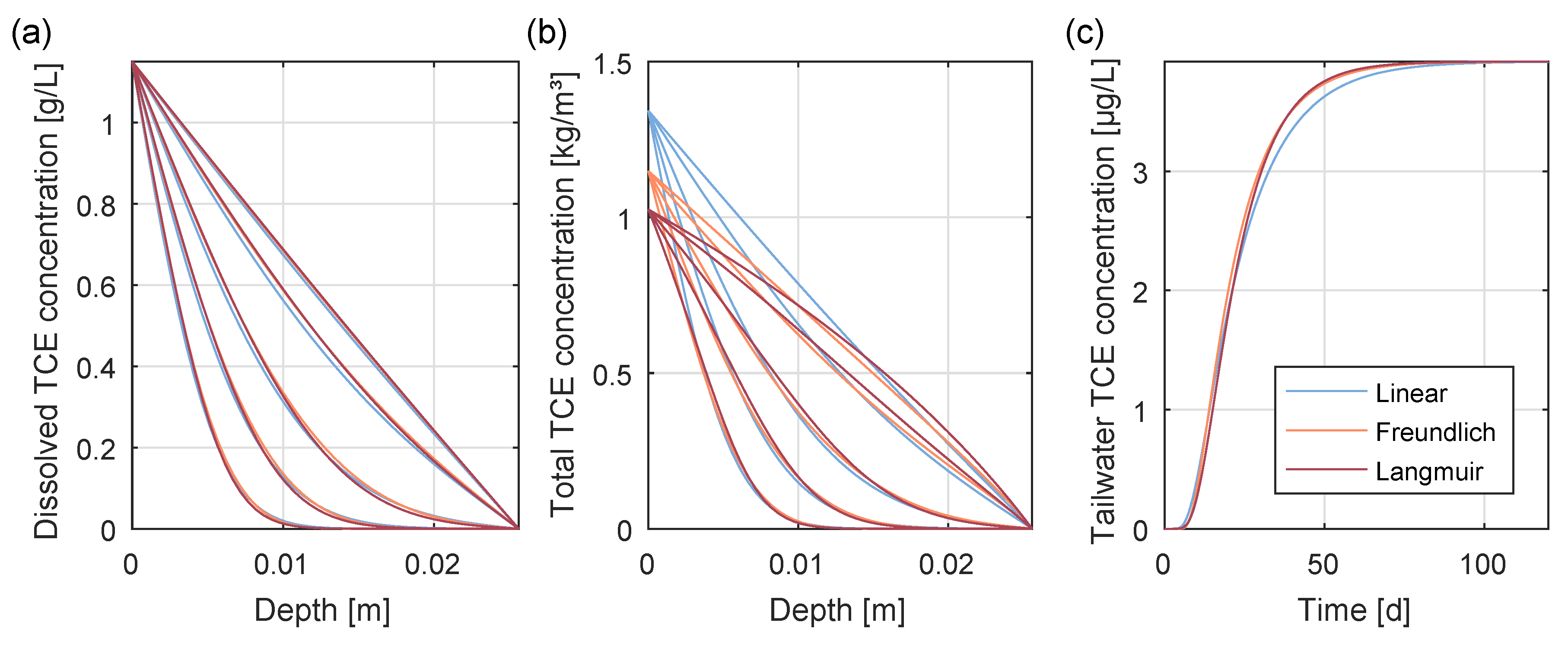
  • Sorption is often assumed to be a sufficiently fast mechanism compared to diffusion, so that sorbed concentrations and dissolved concentrations are always in local equilibrium. Then, sorption may be described by so-called sorption isotherms. There are many different sorption isotherm models available [6], and this is the uncertain model choice we are featuring here.
  • Most sorption isotherms are parametric models. The corresponding inherent parametric uncertainty poses a nuisance in all model identification endeavors. Recognized ways to construct prior estimates for sorption parameters exist only for the so-called linear isotherm model. Prior estimates are based on the fraction of organic matter and other properties of the sorbent (here: clay) and on easily available literature values on the equilibrium of TCE between water and organic reference chemicals [91].
  • There are further challenges: the molecular diffusion coefficients for dissolved chemicals in water are unclear in the literature [92,93,94]. Additionally, the effective diffusion in clay is reduced by two uncertain factors, which are the porosity and the tortuosity of the clay [95]. Porosity is the fraction of void space in the pores to a total volume of clay, and tortuosity measures the excess length of curvilinear paths through the porous medium relative to the straight paths along which transport processes can act in pure water.
  • There are diverging literature values for the solubility of TCE in water [96,97]. Solubility dictates the maximum possible dissolved concentration that occurs when TCE dissolves from the pool into the underlying water-filled pores of the clay, and these concentrations are the driving force for diffusion and sorption.
In order to address the posed model choice problem between sorption isotherms, we use a diffusion cell experiment motivated by Nowak [70]. The experiment is described in Section 3.1. To account for the mentioned uncertainties, we take a probabilistic approach and provide in Section 3.3 a statistical formulation as input for the mathematical model of this experiment (Section 3.2). The definition of the objective function(s) for OD, tailored to this specific experiment, is given in Section 3.4. Finally, results of this case study are presented and discussed in Section 4.

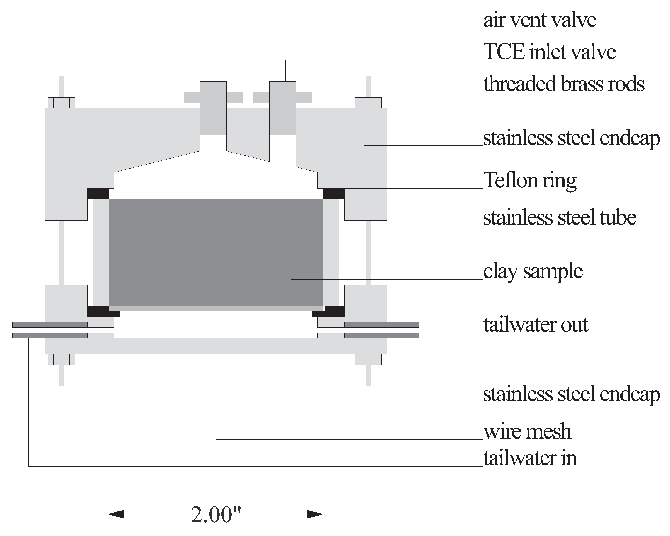
3.1. Experimental Setup and Sampling Design

The experimental setup is depicted in Figure 2. An undisturbed sample of clay is enclosed in a stainless steel tube with length L and inner radius r of 2.54 cm (1 inch); i.e., with an inner diameter of 5.08 cm (2 inches).
Both ends of the tube are closed with Teflon rings and end caps so that small volumes of void space remain. Threaded brass rods hold the sample in place. In the upper void space, a pool of pure TCE is formed by injecting the compound through a dedicated inlet valve, and the corresponding excess air is released through a vent valve. Then, both valves are closed. The bottom void space is free of air. It is constantly flushed with clean water at a controlled flow rate of 5 mL/h. This allows water samples to be taken from the tailwater outlet at regular time intervals. The bottom of the clay core sample is contained with a fine stainless steel mesh. The concentration of dissolved TCE in the tailwater samples is indicative of the progress of diffusion from the top reservoir through the clay core sample to the bottom reservoir, retarded by sorption. After a certain experimental duration T (to be determined by OD), the experiment is stopped, the clay core sample is taken out, and is cut into four horizontal slices of 6.35 mm thickness each (1/4 inch). In these four slices, the total concentration of TCE (dissolved in the pore water plus sorbed onto the clay material) is determined. Details on how such an experiment could be conducted in practice, including the chemical analysis for TCE in water and clay samples, can be found in Nowak [70] and Parker et al. [90].

3.2. Mathematical Model Formulation

The experimental setup is modelled as a one-dimensional system along the vertical axis ( z ) , defined positive in the downward vertical direction. The one-dimensional diffusion equation in a homogeneous porous medium is:
R c t = D e 2 c z 2 ,
here subject to an upper boundary condition provided by the solubility limit c sol :
c ( z = 0 ) = c sol t : 0 t T ,
and a third-type (Cauchy) condition at z = L that results from the flushing with clean water. The initial condition is:
c ( t = 0 ) = 0 z : 0 < z L .
In Equation (22), R [ - ] is the retardation factor due to sorption, c [ M / L 3 ] is the TCE concentration in the pore water, and D e [ L 2 / T ] is the effective porous-medium diffusion coefficient. D e —as appearing in Equation (22)—is related to the molecular diffusion coefficient D m [ L 2 / T ] according to:
D e = D m τ D m · n e ,
where τ [ - ] is tortuosity and n e is an effective porosity. The above approximation is based on the assumption that τ 1 / n e .
The retardation factor is defined by:
R = 1 n e c t c ,
where c t [ M / L 3 ] is the total concentration (dissolved and sorbed) with respect to bulk volume of porous medium [98]:
c t = n e c + ( 1 - n e ) ρ s s ( c ) .
Here, ρ s [ M / L 3 ] is the density of solids that constitute the porous medium, and s ( c ) [ M / M ] is the mass of sorbed compound per solids mass, at equilibrium with a given value of dissolved concentration c.
The sorbed concentration s is most often parameterized by one of the following three isotherms:
(28) s ( c ) = K d c     linear (29) s ( c ) = K c n f     Freundlich (30) s ( c ) = s max c c + K     Langmuir .
These are called the linear, Freundlich, and Langmuir isotherms [99]. Figure 3 illustrates the three isotherms. For the sake of demonstrating problems with model identification, Figure 3 shows parameter configurations for each isotherm that yield very similar curves in the lower range of concentrations (0–0.5 g/L).
In the linear isotherm, K d [ L 3 / M ] is called the partitioning coefficient, and it can be estimated by:
K d = f OC K OC ,
where f OC [ - ] is the mass fraction of organic carbon in the solids and K OC [ L 3 / M ] is the partitioning coefficient of the compound of interest between organic matter and water. Often, the value for partitioning between octanol and water, K OW , is used to estimate K OC . Here, we are only interested in estimating the product of both f OC and K OC (i.e., K d ). The Freundlich isotherm is an empirical extension of the linear case to a power-law-type relation, using the exponent n f [ - ] . We use here the subscript f to indicate Freundlich and to differentiate it from the notation for porosity. Note that for n f = 1 , the Freundlich model collapses to the linear model. In this sense, the two models are nested models. The Langmuir isotherm is motivated through a mechanistic model of sorption, where s max [ M / M ] denotes the maximum sorption capacity of the sorbent, and K is the so-called half-saturation value (i.e., the value of c where s attains half of its maximum value s max [99]).
The resulting expressions for R are [99]:
(32) R = 1 + 1 - n e n e ρ s K d     linear (33) R = 1 + 1 - n e n e ρ s K n f c n f - 1     Freundlich (34) R = 1 + 1 - n e n e ρ s s max K ( c + K ) 2     Langmuir
When plugging any of these three retardation factors into the diffusion equation, we obtain three competing models, which we wish to differentiate through experimentation. We solve the resulting (non-linear) partial differential equations with a central finite difference scheme in space, and an explicit finite difference scheme in time. The spatial and temporal resolution chosen is Δ z = 0 . 05   m and Δ t = 450   s . This is fine enough to ensure the insensitivity of all subsequent results to any remaining numerical approximation errors.
Figure 4a,b illustrate the dissolved and total TCE concentrations, respectively, that can be found in the clay core sample at different points in time. Figure 4c shows an exemplary time series of TCE concentrations that could be observed in the water samples every 24 h. This time series is referred to as breakthrough curve (BTC) in the following. The actual values chosen for the parameter values do not matter here, as they merely serve for illustration. In fact, they are realizations drawn from the prior distributions introduced in the following section.

3.3. Statistical Formulation

Between the three competing models, we assume an uninformative prior distribution of model weights (i.e., all prior model weights are equal to one third). This resembles a typical preference-free starting point of model choice. Allen-King et al. [100] found that the sorption of TCE in four clayey formations can be represented reasonably well by a Freundlich isotherm. However, this is a relatively small number of examples, and we continue with the non-informative prior for the sake of illustration.
Finding prior distributions for all uncertain model parameters in each model is a less trivial task in our featured case. An established mechanism for estimating model parameters without conducting direct sorption experiments exists only for the linear sorption isotherm. Thus, at first, we determine probability distributions for the linear isotherm model. Then, we find prior distributions for the parameters of the other two models by fitting them to relevant aspects of the prior predictive distribution for the random BTCs that result from the linear isotherm model.
Our assumptions for the prior parameter distributions in the linear isotherm model are based on soil data taken from Nowak [70], and on specific considerations that are explained in Appendix A. The resulting distributions are listed in Table 1.
For the parameter distributions of the Freundlich and Langmuir isotherms, we aimed at a maximal similarity of the resulting ensemble of BTCs, simulated with all three models. Thus, we ran a Monte Carlo simulation of the linear model and used the first temporal moments [101] of the resulting ensemble to define the similarity of BTCs. The first temporal moment of a unit-pulse-input system response is the product of a characteristic response strength and a characteristic response time. We took the temporal derivatives of the BTCs before computing their first temporal moments in order to convert them to the equivalent of a unit-pulse system response.
Then, we constructed a Monte Carlo Markov Chain (MCMC) with Metropolis–Hastings sampling [102]. The MCMC has the purpose of producing distributions for all parameter values of the Freundlich and Langmuir isotherms that yield BTCs with the same distribution of first temporal moments. To achieve this, we start from a non-informative prior for all parameters in the Freundlich and Langmuir isotherms, and define the likelihood for Bayesian updating as the product of the probability density values of all common parameters (porosity, density, solubility, molecular diffusion, cf. Table 1) and the probability density value in the empirical distribution of first moments for the linear isotherm provided by the Monte Carlo simulation.
The resulting predictive distributions (expected values and Bayesian credible intervals) for the three sorption models are shown in Figure 5. The predictions of total TCE concentration in the bottom clay slice differ visibly after an experimental duration of about 14 days. In contrast, the predictions of tailwater TCE concentration are much harder to distinguish, and show a window between the fifth and the 30th day, where model predictions seem to disagree the most.
The predictive distributions obtained from the MCMC serve as prior distributions p Y k | M k that shall be updated to model-specific posterior distributions p Y k | y o , M k and to a BMA-weighted combination p Y | y o via Equation (2). Here, we assume the likelihood function p y o | s k , M k needed in Equations (5) and (7) to be Gaussian with a measurement error covariance matrix C ϵ :
p y o | M k , s k = 2 π - N s / 2 C ϵ - 1 / 2 exp - 1 2 y o - y k T C ϵ - 1 y o - y k .
The diagonal matrix C ϵ has a size of N s × N s , with N s being the number of data points in y o according to the design d. As measurement errors, we choose a relative error of 5 % of the measurement values as standard deviation, plus an absolute error of 2 × 10 - 7 kg/m 3 in the case of TCE concentrations in the tailwater and of 1 × 10 - 4 kg/m 3 in the case of total concentrations in the clay slices.
With the updated model probabilities and posterior predictive distributions, we can determine D KL (Equation (14)) and the total model-averaged prediction variance V Y | y o (Equation (4)) for any specific data set y o .

3.4. Formulation and Implementation of the Optimal Design Problem

To specifically address the conceptual uncertainty about which sorption model most adequately describes the transport behaviour of TCE through the clay core sample, we define the OD objective function as the mutual information I ( X ; Y d ) between possible data Y d and model choice indicators X (Equation (18)). The longer the experiment is conducted, the more tailwater samples can be collected, and the more information they can provide. However, the later the clay slices are analyzed, the more the system has approached a steady state where the spatial distribution of TCE in the clay core sample is less affected by sorption. Therefore, the total experimental duration is a compromise between expected information gain from the water samples and from the clay samples. The total experimental duration is the variable we will optimize through OD in our example, restricted to a maximum feasible duration of 120 days.
For comparison, we also consider as OD objective the reduction in predictive variance V red Z | Y d (Equation (20)) of the tailwater BTC from T = 0 to T = 120 days. The possible data Y d contain both water and clay samples, while their utility will be measured with regard to uncertainty in water concentrations only. Hence, in this case, Z Z Y .
Details about the numerical implementation are provided in Appendix B.

4. Results and Discussion

Two exemplary posterior predictive distributions of the BTC are shown in Figure 6. They result from conditioning on two different exemplary data sets, (for the moment) arbitrarily chosen from the ensemble of possible data sets used for the preposterior analysis. Through conditioning, the 95% credible intervals have shrunk as compared to the prior situation in Figure 5b. The remaining differences between the models after conditioning will be discussed later in detail.
The outcome of model weights after conditioning on the data set underlying Figure 6a is shown in Figure 1b (dark green circle). Model choice uncertainty has been successfully reduced from the state of maximum entropy (equal prior model weights) to a posterior state with model weights of 85%, 15% and 0% for the linear, Freundlich, and Langmuir models, respectively. For each proposed design, we have simulated many possible outcomes of sampling data during the preposterior analysis (see Appendix B for details). The green circles in Figure 1b represent the corresponding possible outcomes of model weights for the same design. As compared to a less informed state (gray circles), the entropy of model weights has been significantly reduced (the circles have moved towards the edges and vertices of the triangle). From the distribution of the green circles in the ternary plot, it can further be concluded that the linear model can be easily distinguished from the Langmuir model (in the case when the Freundlich model receives a weight of zero, bottom horizontal edge). However, there is a less decisive weighting between the Freundlich and the Langmuir model (when the linear model receives a weight of zero, left edge). Additionally, the linear model tends to be preferred over the more complex (i.e., with one additional parameter) Freundlich model (when the Langmuir model receives a weight of zero, right edge). This is due to the implicit characteristic of BMS to prefer simpler models under limited data set sizes if differences in performance are reasonably small (e.g., [87]).
Figure 7a shows the values of the objective functions I ( X ; Y d ) (left axis) and V red Z | Y d (right axis) plotted over the experimental duration from T = 0 to T = 120 days. As opposed to data worth with respect to total variance reduction, mutual information does not increase monotonically with experimental duration. Instead, it shows a local and a global maximum before it flattens out. This behaviour can be explained by looking at the data worth of tailwater samples (dashed line) and clay slice samples (dashed-dotted line) individually: the cumulative data worth of water samples increases with time, because more samples are consecutively added with increasing experimental duration. Clay samples, however, are only taken at the end of the experiment. Thus, the curve shown in Figure 7a for clay samples does not represent a cumulative data worth, but the one-time data worth at the respective end of the experiment. This is why their data worth varies non-monotonically, has a global maximum at seven days, a local minimum at 14 days, and then rises again to an almost constant level. The combined information content of water and clay samples represents a compromise of both, and yields an optimum at 23 days (marked by a vertical green line in Figure 5, Figure 6a, and Figure 7a). This optimum state is also shown by the green circles in the ternary plot in Figure 1b. The maximum value of mutual information ( I = 0.5886 ) corresponds to the reduction of entropy by moving from the prior state of knowledge (black circle, H = - ln 1 3 = 1.0986 ) to the posterior state with a conditional (remaining) entropy of H = 0.5100 .
The data worth for model choice can be further investigated by asking: how well can a model recognize itself if it had actually generated the data? We refer to this as the self-identification probability (see also Schöniger et al. [87]). The models’ self-identification probability is shown as a function of experimental duration in Figure 7b. Again, the solid lines represent the combined information provided by water and clay samples, while the dashed–dotted line refers to the information in clay samples alone. It becomes clear that the peak in mutual information between model choice and clay concentration data is mainly due to the self-identification potential of the linear model, as it shows a very similar curve. It is indeed to be expected that the simplest model (here: the linear) achieves the highest self-identification probability, due to the implicit characteristic of BMS to favour more parsimonious models. In contrast, the Freundlich model suffers from the fact that it is quite similar to the simpler linear model (for n f 1 , it approaches the linear model), and hence, when in doubt, BMS prefers the linear model over the Freundlich model unless sorption is clearly non-linear. This is why the Freundlich model is limited to a maximum self-identification probability that is approximately 20%–30% lower than for the other two models.
The self-identification probabilities also underpin why a sampling end time of 23 days is optimal with respect to model choice—all three models then have a (close-to-)maximum chance of being correctly identified if they were actually the true model.
The self-identification probabilities based on consecutive water samples hardly increase after approximately 60 days. This is due to the fact that all models are able to fit the observed tailwater concentrations very well in the late stage (steady state) of the experiment (cf. Figure 6b), such that it becomes practically impossible to distinguish between the three sorption models. Additional observations mostly carry redundant information, and can only help reduce the diluting impact of measurement noise—they can no longer significantly contribute to model discrimination.
If the goal is to reduce the total predictive uncertainty, the experiment should be run for as long as possible. The reason is that data worth with respect to variance reduction increases monotonically with experimental duration (after a local maximum at eight days, cf. Figure 7a). This result is intuitive, because the optimization target is the uncertainty in the predicted BTC in the tailwater; the more water samples we gather (dashed black line), the higher the uncertainty reduction. However, it also becomes obvious that clay samples at an early stage of diffusion through the clay core sample are much more informative about the breakthrough in the tailwater than those at later times.
The effect of optimizing towards the two competing objectives (1) decisiveness in model choice, and (2) total predictive uncertainty can be seen in Figure 6: the resulting predictions shown in Figure 6a originate from the optimal design according to objective (1), while the predictions shown in Figure 6b originate from the optimal design according to objective (2). In Figure 6a, within-model variance and between-model variance are larger than in Figure 6b. Yet, the individual models are visibly distinguishable, which was the purpose of the design. On the right, the predictive distributions practically overlay each other, such that the total uncertainty is slightly smaller; however, the models can hardly be discriminated. Note that as the linear model receives a high weight of 85 % in this particular example, its curves are obscured behind the BMA mean and BMA credible intervals in the left graph.
The competition between objectives (1) and (2) is analyzed in Figure 8. It becomes obvious that, up to 90% uncertainty reduction and a mutual information of 0.5 , there is actually no trade-off between the two objectives. In this range of designs, an improvement in one of the two objectives also leads to an improvement in the other one. However, towards the maxima of both objective functions, an oddly-shaped trade-off behaviour begins to emerge (inset of Figure 8). This means that to obtain optimal results, we need to decide for one of the two objectives; however, an almost-optimal compromise solution could also be found without too much remorse by performing multi-objective OD (e.g., [103]).

5. Summary and Conclusions

In this study, we have addressed the problem of model choice uncertainty that is common in the field of geosciences. We did so by advancing an approach to optimal experimental design (OD) specifically tailored to model selection. OD for future data collection can help to increase the decisiveness of model selection techniques. Here, we adopt the methodology of Bayesian model selection (BMS) to update a prior belief about the adequacy of competing conceptual models to a posterior model probability in the light of (newly gained) data. The goal of experimentation is to achieve a maximal expected information gain through additional data towards the decisiveness in model ranking. Following earlier studies from the field of statistics [58,59], we use the mutual information between model choice indicators and the possible outcomes of future data as the objective function to be optimized. We implement this preposterior analysis with the PreDIA scheme by Leube et al. [69].
Compared to the existing methods that can be found in the geosciences and statistics, our framework combines several advantages: (1) it benefits from a rigorous and consistent formulation of entropy-based OD for model choice that builds on the concept of model choice indicators. (2) It is free of any lower-order approximations. (3) It can handle arbitrary data types and uncertainty in future data due to parameter uncertainty and measurement error. (4) It can be applied for both sequential and global designs.
We have illustrated our methodology with an application to contaminant transport in the subsurface, namely trichloroethylene (TCE) sorption and diffusion through a clay core sample. In order to identify one of three plausible sorption isotherm models (i.e., the linear, Freundlich, or Langmuir model), a diffusion cell experiment is to be planned. Concentrations of dissolved TCE in tailwater samples (taken once per day until the end of the experiment), and total TCE concentrations (dissolved plus sorbed) in clay samples (taken after ending the experiment) provide information on the transport of TCE through the clay core sample, and hence on the sorption behaviour. We have applied our advanced framework for OD to identify the optimum experimental duration that yields a maximum reduction in model choice uncertainty. For the sake of comparison with alternative formulations of OD in the presence of model choice uncertainty, we have also investigated the optimum experimental duration when the goal is to minimize the total model-averaged predictive uncertainty of the breakthrough curve (BTC) in the tailwater. In the latter case, the model choice problem is only implicitly addressed, while our favoured OD formulation tackles it directly via the model choice indicators.
We have presented several options for analyzing the quality of proposed designs; for example, by visualizing the remaining model choice uncertainty in a ternary plot (reflecting the preposterior nature of model-based OD) or by investigating the self-identification probability of the competing models.
Our results have shown that mutual information with respect to model choice does not increase monotonically with experimental duration, as opposed to data worth with respect to total variance reduction. There is a trade-off between the cumulative data worth of sequential water samples (which increases over time) and the data worth of individual clay samples (which is higher at earlier stages of the experiment), because the later steady state concentration profile in the clay core sample is less informative about sorption isotherms. In general, the data worth also depends greatly on the quality of the measurements. Assumptions about measurement accuracy are accounted for by BMS, and hence are reflected by the resulting optimal design. The optimal design identified here would have been non-trivial to find without a formal optimization, since there are many factors involved that influence the decisiveness in model choice in complicated, interacting ways.
Hence, when confronted with relevant model choice uncertainty, we recommend an optimization based on the OD formulation presented in this study in order to get the most out of an experiment. Our comparison has shown that the two alternative design objectives—decisiveness in model choice and reduction of total predictive uncertainty—are (at least in our case study) only partially conflicting. By identifying the trade-off characteristics, modellers and experimenters can decide how to best design an experiment, such that the specific scientific goals can be achieved in a timely and cost-efficient manner.

Acknowledgments

The authors would like to thank the German Research Foundation (DFG) for financial support of the project within the Cluster of Excellence in Simulation Technology (EXC 310/1) at the University of Stuttgart and within the International Research Training Group “Integrated Hydrosystem Modelling” (IRTG 1829) at the University of Tübingen. The authors received support by the DFG and the Open Access Publishing Fund of the University of Tübingen for covering the costs to publish in open access. The diffusion cell setup and the specific problem of model choice has its roots in the Master’s thesis of Wolfgang Nowak back in 1999–2000. In this context, Wolfgang Nowak would like to express his sincere gratitude to his former supervisors Beth L. Parker and John Cherry, and to the field/lab crew at the University of Waterloo, Ontario, Canada. The authors would further like to thank Jeremy Bennett from the University of Tübingen and three anonymous reviewers for very constructive comments that helped improve this manuscript.

Author Contributions

Both authors have substantially contributed to this work, from conceiving the idea of specifically addressing conceptual uncertainty in optimal experimental design by measuring the entropy of model choice indicators to implementing the presented case study. Both authors have been involved in writing and revising the paper, and they have both read and approved the submitted version of the manuscript.

Conflicts of Interest

The authors declare no conflict of interest.

Abbreviations

The following abbreviations are used in this manuscript:
BMABayesian model averaging
BMEBayesian model evidence
BMSBayesian model selection
BTCBreakthrough curve
DNAPLDense non-aqueous phase liquid
KLKullback–Leibler
MCMCMonte Carlo Markov Chain
ODOptimal experimental design
PreDIAPreposterior Data Impact Assessor
TCETrichloroethylene

Appendix A. Additional Considerations for the Statistical Formulation of the Case Study

To determine the prior parameter distributions for the linear isotherm model, we have drawn on the following considerations:
  • Per definition, we find that porosity n e [ 0 , 1 ] , so that we choose the beta distribution. Multiple measurements of porosity for the specific clay formation analyzed in Nowak [70] indicate that n e 0.3 . Based on sample statistics, we assign a 95 % credible interval of 0.3 ± 0.02 . The resulting parameters of the chosen parametric distribution for porosity (and also for all of the following quantities) are shown in Table 1.
  • Densities are non-negative per definition. Thus, we choose a lognormal distribution for the solids density of the featured clay. The featured density is slightly higher than that of Quartz (with ρ Quartz = 2650 kg/m 3 ). Sample statistics indicate a modal value of ρ s = 2895 kg/m 3 and a 50 % credible interval of 2895 ± 15 kg/m 3 .
  • Solubilities are upper bounds for concentrations and hence non-negative, leading us to the lognormal distribution. TCE solubility experiments with site-specific groundwater indicated a modal value of c sol = 1400   mg / L and a 95 % credible interval of 1400 ± 27   mg / L .
  • Molecular diffusion coefficients D m are once again non-negative quantities, so we again use the lognormal distribution. For TCE, the different values that can be found in literature suggest for us to choose a 95 % credible interval of 6.155 ± 0.475 m 2 /s.
  • The distribution of D e follows implicitly through Equation (25).
  • The distribution for the partitioning coefficient K d in the linear isotherm follows from Equation (31); i.e., we need to define distributions for f OC and K OC .
  • f OC is a fraction in the interval [ 0 , 1 ] , leading to the beta distribution. The available single datum is f OC = 0.269 % , with an estimated (by subjective expert opinion) coefficient of variation that is half of the measured value.
  • K OC is non-negative and hence lognormal. Schwarzenbach and Westall [104] provide a range of values that leads us to choose a 95 % credible interval of 132.5 ± 38.5 mL/kg.

Appendix B. Numerical Implementation of OD in the Case Study

We perform Bayesian updating from prior parameter realizations s k , i (obtained from the MCMC, see Section 3.3), with i = 1     N M C , to posterior realizations by weighting each realization with its respective likelihood p y o | s k , i , M k . This Monte Carlo implementation of Bayesian updating is known as weighted bootstrap [105].
BME is determined from Monte Carlo integration of Equation (7); i.e., by averaging over the likelihoods of the N MC realizations in the prior ensemble:
p y o | M k 1 N M C i = 1 N M C p y o | s k , i , M k .
Upon evaluation of BME, and with the assumption of equal prior model weights, posterior model weights needed for D KL and V Y | y o can be inferred via Equation (6).
We use N MC = 50 , 000 prior realizations per model. Additionally, N PP , k = 1000 realizations of predictions are generated per model as possible data sets for the preposterior analysis. In total, this sums up to N PP = 3000 data sets to be considered in PreDIA [69], and a total number of N MC × N PP   =   1.5 × 10 8 evaluations of the likelihood function per model. The PreDIA engine automatically considers the random measurement errors of predicted data according to Equation (15).
Average effective sample sizes [69] between 476 and 10 , 651 and visual inspection of the results indicate that convergence has been achieved. Note that while our study features a first-time implementation of PreDIA for Bayesian model weights, this algorithm is similar to the random sampling of measurement error for analyzing the robustness of BMA results, as presented in Schöniger et al. [106]. A related schematic illustration of the implementation scheme can be found there. All calculations for the current study were carried out in MATLAB on a contemporary desktop computer.
Finally, we need to obtain the two target quantities for optimization considered in this study; i.e., mutual information I ( X ; Y d ) (Equation (16)) and the expected reduction in total predictive variance V red Z | Y d (Equation (21)). Both quantities are obtained by averaging over data realizations j, with j = 1     N PP . We find the optimal design with respect to model choice, d opt , X , or with respect to total predictive variance, d opt , V , by identifying the experimental duration with maximum I ( X ; Y d ) or maximum V red Z | Y d , respectively. The optimization problem featured here is relatively simple, so we solve it by exhaustive enumeration of all 121 admissible designs, ranging over an experimental duration of T = 0 , 1 , , 120 days.

References

  1. Winsberg, E. Simulated Experiments: Methodology for a Virtual World. Philos. Sci. 2003, 70, 105–125. [Google Scholar] [CrossRef]
  2. Beven, K.J. Uniqueness of place and process representations in hydrological modelling. Hydrol. Earth Syst. Sci. 2000, 4, 203–213. [Google Scholar] [CrossRef]
  3. Christie, M.A.; Blunt, M.J. Tenth SPE Comparative Solution Project: A Comparison of Upscaling Techniques. SPE Res. Eval. Eng. 2001, 4, 308–317. [Google Scholar]
  4. Oreskes, N.; Shrader-Frechette, K.; Belitz, K. Verification, validation, and confirmation of numerical models in the earth sciences. Science 1994, 263, 641–646. [Google Scholar] [CrossRef] [PubMed]
  5. Neuman, S.P.; Tartakovsky, D.M. Perspective on theories of non-Fickian transport in heterogeneous media. Adv. Water Resour. 2009, 32, 670–680. [Google Scholar] [CrossRef]
  6. Limousin, G.; Gaudet, J.P.; Charlet, L.; Szenknect, S.; Barthès, V.; Krimissa, M. Sorption isotherms: A review on physical bases, modeling and measurement. Appl. Geochem. 2007, 22, 249–275. [Google Scholar] [CrossRef]
  7. Wang, N.; Brennan, J.G. Moisture sorption isotherm characteristics of potatoes at four temperatures. J. Food Eng. 1991, 14, 269–287. [Google Scholar] [CrossRef]
  8. Joekar-Niasar, V.; Hassanizadeh, S.M.; Leijnse, A. Insights into the Relationships Among Capillary Pressure, Saturation, Interfacial Area and Relative Permeability Using Pore-Network Modeling. Transp. Porous Media 2008, 74, 201–219. [Google Scholar] [CrossRef]
  9. Lötgering-Lin, O.; Gross, J. Group Contribution Method for Viscosities Based on Entropy Scaling Using the Perturbed-Chain Polar Statistical Associating Fluid Theory. Ind. Eng. Chem. Res. 2015, 54, 7942–7952. [Google Scholar] [CrossRef]
  10. Beven, K. Causal models as multiple working hypotheses about environmental processes. C. R. Geosci. 2012, 344, 77–88. [Google Scholar] [CrossRef]
  11. Beven, K. Towards a coherent philosophy for modelling the environment. Proc. R. Soc. Lond. A Math. Phys. Eng. Sci. R. Soc. 2002, 458, 2465–2484. [Google Scholar] [CrossRef] [Green Version]
  12. Luis, S.J.; McLaughlin, D. Validation of Geo-hydrological Models: Part 1. A stochastic approach to model validation. Adv. Water Resour. 1992, 15, 15–32. [Google Scholar] [CrossRef]
  13. Walker, W.E.; Harremoës, P.; Rotmans, J.; van der Sluijs, J.P.; van Asselt, M.B.A.; Janssen, P.; Krayer von Krauss, M.P. Defining Uncertainty: A Conceptual Basis for Uncertainty Management in Model-Based Decision Support. Integr. Assess. 2003, 4, 5–17. [Google Scholar] [CrossRef]
  14. Bernardo, J.M.; Rueda, R. Bayesian Hypothesis Testing: a Reference Approach. Int. Stat. Rev. 2002, 70, 351–372. [Google Scholar] [CrossRef]
  15. Raftery, A.E. Bayesian Model Selection in Social Research. Sociol. Methodol. 1995, 25, 111–163. [Google Scholar] [CrossRef]
  16. Huelsenbeck, J.P.; Larget, B.; Alfaro, M.E. Bayesian Phylogenetic Model Selection Using Reversible Jump Markov Chain Monte Carlo. Mol. Biol. Evol. 2004, 21, 1123–1133. [Google Scholar] [CrossRef] [PubMed]
  17. Hoeting, J.A.; Madigan, D.; Raftery, A.E.; Volinsky, C.T. Bayesian model averaging: A tutorial. Stat. Sci. 1999, 14, 382–401. [Google Scholar]
  18. Najafi, M.R.; Moradkhani, H.; Jung, I.W. Assessing the uncertainties of hydrologic model selection in climate change impact studies. Hydrol. Proc. 2011, 25, 2814–2826. [Google Scholar] [CrossRef]
  19. Seifert, D.; Sonnenborg, T.O.; Refsgaard, J.C.; Højberg, A.L.; Troldborg, L. Assessment of hydrological model predictive ability given multiple conceptual geological models. Water Resour. Res. 2012, 48, W06503. [Google Scholar] [CrossRef]
  20. Tsai, F.T.C.; Elshall, A.S. Hierarchical Bayesian model averaging for hydrostratigraphic modeling: Uncertainty segregation and comparative evaluation. Water Resour. Res. 2013, 49, 5520–5536. [Google Scholar] [CrossRef]
  21. Rojas, R.; Feyen, L.; Dassargues, A. Conceptual model uncertainty in groundwater modeling: Combining generalized likelihood uncertainty estimation and Bayesian model averaging. Water Resour. Res. 2008, 44. [Google Scholar] [CrossRef]
  22. Troldborg, M.; Nowak, W.; Tuxen, N.; Bjerg, P.L.; Helmig, R.; Binning, P.J. Uncertainty evaluation of mass discharge estimates from a contaminated site using a fully Bayesian framework. Water Resour. Res. 2010, 46. [Google Scholar] [CrossRef]
  23. Ye, M.; Pohlmann, K.F.; Chapman, J.B.; Pohll, G.M.; Reeves, D.M. A model-averaging method for assessing groundwater conceptual model uncertainty. Ground Water 2010, 48, 716–728. [Google Scholar] [CrossRef] [PubMed]
  24. MacKay, D.J.C. Bayesian Interpolation. Neural Comput. 1992, 4, 415–447. [Google Scholar] [CrossRef]
  25. Neretnieks, I. Diffusion in the rock matrix: An important factor in radionuclide retardation? J. Geophys. Res. Solid Earth 1980, 85, 4379–4397. [Google Scholar] [CrossRef]
  26. Frster, A.; Norden, B.; Zinck-Jrgensen, K.; Frykman, P.; Kulenkampff, J.; Spangenberg, E.; Erzinger, J.; Zimmer, M.; Kopp, J.; Borm, G. Baseline characterization of the CO2SINK geological storage site at Ketzin, Germany. Environ. Geosci. 2006, 13, 145–161. [Google Scholar] [CrossRef]
  27. Pukelsheim, F.; Rosenberger, J.L. Experimental Designs for Model Discrimination. J. Am. Stat. Assoc. 1993, 88, 642–649. [Google Scholar] [CrossRef]
  28. Christakos, G. Random Field Models in Earth Sciences; Dover Publications, Inc.: Mineola, NY, USA, 2012. [Google Scholar]
  29. Fishburn, P.C. Utility Theory for Decision Making; Publications in Operations Research; Wiley: New York, NY, USA, 1970; Volume 18. [Google Scholar]
  30. Lindley, D.V. Bayesian Statistics: A Review; SIAM: Philadelphia, PA, USA, 1972. [Google Scholar]
  31. Abellan, A.; Noetinger, B. Optimizing subsurface field data acquisition using information theory. Math. Geosci. 2010, 42, 603–630. [Google Scholar] [CrossRef]
  32. Nowak, W.; de Barros, F.P.J.; Rubin, Y. Bayesian geostatistical design: Task-driven optimal site investigation when the geostatistical model is uncertain. Water Resour. Res. 2010, 46. [Google Scholar] [CrossRef]
  33. Kollat, J.B.; Reed, P.M.; Maxwell, R.M. Many-objective groundwater monitoring network design using bias-aware ensemble Kalman filtering, evolutionary optimization, and visual analytics. Water Resour. Res. 2011, 47. [Google Scholar] [CrossRef]
  34. Freeze, R.A.; James, B.; Massmann, J.; Sperling, T.; Smith, L. Hydrogeological Decision-Analysis: 4. The Concept of Data Worth and Its Use in the Development of Site Investigation Strategies. Ground Water 1992, 30, 574–588. [Google Scholar] [CrossRef]
  35. James, B.R.; Gorelick, S.M. When Enough Is Enough: The Worth of Monitoring Data in Aquifer Remediation Design. Water Resour. Res. 1994, 30, 3499–3513. [Google Scholar] [CrossRef]
  36. Berger, J.O. Statistical Decision Theory and Bayesian Analysis; Springer Science & Business Media: New York, NY, USA, 2013. [Google Scholar]
  37. Box, G.E.; Tiao, G.C. Bayesian Inference in Statistical Analysis; John Wiley & Sons: New York, NY, USA, 2011; Volume 40. [Google Scholar]
  38. Chaloner, K.; Verdinelli, I. Bayesian experimental design: A review. Stat. Sci. 1995, 10, 273–304. [Google Scholar] [CrossRef]
  39. Cover, T.M.; Thomas, J.A. Entropy, relative entropy and mutual information. Elem. Inf. Theory 1991, 2, 1–55. [Google Scholar]
  40. Cirpka, O.A.; Burger, C.M.; Nowak, W.; Finkel, M. Uncertainty and data worth analysis for the hydraulic design of funnel-and-gate systems in heterogeneous aquifers. Water Resour. Res. 2004, 40. [Google Scholar] [CrossRef]
  41. Sciortino, A.; Harmon, T.C.; Yeh, W.W.G. Experimental design and model parameter estimation for locating a dissolving dense nonaqueous phase liquid pool in groundwater. Water Resour. Res. 2002, 38, 15-1–15-9. [Google Scholar] [CrossRef]
  42. Altmann-Dieses, A.E.; Schlöder, J.P.; Bock, H.G.; Richter, O. Optimal experimental design for parameter estimation in column outflow experiments. Water Resour. Res. 2002, 38, 4-1–4-11. [Google Scholar] [CrossRef]
  43. Vrugt, J.A.; Bouten, W.; Gupta, H.V.; Sorooshian, S. Toward improved identifiability of hydrologic model parameters: The information content of experimental data. Water Resour. Res. 2002, 38. [Google Scholar] [CrossRef]
  44. Müller, W.G. Collecting Spatial Data: Optimum Design of Experiments for Random Fields; Springer Science & Business Media: New York, NY, USA, 2007. [Google Scholar]
  45. McKinney, D.C.; Loucks, D.P. Network design for predicting groundwater contamination. Water Resour. Res. 1992, 28, 133–147. [Google Scholar] [CrossRef]
  46. Herrera, G.S.; Pinder, G.F. Space-time optimization of groundwater quality sampling networks. Water Resour. Res. 2005, 41. [Google Scholar] [CrossRef]
  47. Janssen, G.M.C.M.; Valstar, J.R.; van der Zee, S.E.A.T.M. Measurement network design including traveltime determinations to minimize model prediction uncertainty. Water Resour. Res. 2008, 44, W02405. [Google Scholar] [CrossRef]
  48. De Barros, F.P.J.; Ezzedine, S.; Rubin, Y. Impact of hydrogeological data on measures of uncertainty, site characterization and environmental performance metrics. Adv. Water Resour. 2012, 36, 51–63. [Google Scholar] [CrossRef]
  49. Neuman, S.P.; Xue, L.; Ye, M.; Lu, D. Bayesian analysis of data-worth considering model and parameter uncertainties. Adv. Water Resour. 2012, 36, 75–85. [Google Scholar] [CrossRef]
  50. Lu, D.; Ye, M.; Neuman, S.P.; Xue, L. Multimodel Bayesian analysis of data-worth applied to unsaturated fractured tuffs. Adv. Water Resour. 2012, 35, 69–82. [Google Scholar] [CrossRef]
  51. Parrish, M.A.; Moradkhani, H.; DeChant, C.M. Toward reduction of model uncertainty: Integration of Bayesian model averaging and data assimilation. Water Resour. Res. 2012, 48. [Google Scholar] [CrossRef]
  52. Xue, L.; Zhang, D.; Guadagnini, A.; Neuman, S.P. Multimodel Bayesian analysis of groundwater data worth. Water Resour. Res. 2014, 50, 8481–8496. [Google Scholar] [CrossRef]
  53. Atkinson, A.C. DT-optimum designs for model discrimination and parameter estimation. J. Stat. Plan. Inference 2008, 138, 56–64. [Google Scholar] [CrossRef]
  54. Wöhling, T.; Schöniger, A.; Gayler, S.; Nowak, W. Bayesian model averaging to explore the worth of data for soil-plant model selection and prediction. Water Resour. Res. 2015, 51, 2825–2846. [Google Scholar] [CrossRef]
  55. Atkinson, A.C.; Fedorov, V.V. Optimal design: Experiments for discriminating between several models. Biometrika 1975, 62, 289–303. [Google Scholar] [CrossRef]
  56. Hill, P.D.H. A Review of Experimental Design Procedures for Regression Model Discrimination. Technometrics 1978, 20, 15–21. [Google Scholar] [CrossRef]
  57. Box, G.E.P.; Hill, W.J. Discrimination among Mechanistic Models. Technometrics 1967, 9, 57–71. [Google Scholar] [CrossRef]
  58. Cavagnaro, D.R.; Myung, J.I.; Pitt, M.A.; Kujala, J.V. Adaptive Design Optimization: A Mutual Information-Based Approach to Model Discrimination in Cognitive Science. Neural Comput. 2010, 22, 887–905. [Google Scholar] [CrossRef] [PubMed]
  59. Drovandi, C.C.; McGree, J.M.; Pettitt, A.N. A Sequential Monte Carlo Algorithm to Incorporate Model Uncertainty in Bayesian Sequential Design. J. Comput. Graph. Stat. 2014, 23, 3–24. [Google Scholar] [CrossRef] [Green Version]
  60. Knopman, D.S.; Voss, C.I. Discrimination among one-dimensional models of solute transport in porous media: Implications for sampling design. Water Resour. Res. 1988, 24, 1859–1876. [Google Scholar] [CrossRef]
  61. Usunoff, E.; Carrera, J.; Mousavi, S.F. Validation of Geo-hydrological ModelsAn approach to the design of experiments for discriminating among alternative conceptual models. Adv. Water Resour. 1992, 15, 199–214. [Google Scholar] [CrossRef]
  62. Hunter, W.G.; Reiner, A.M. Designs for Discriminating Between Two Rival Models. Technometrics 1965, 7, 307–323. [Google Scholar] [CrossRef]
  63. Kikuchi, C.P.; Ferré, T.P.A.; Vrugt, J.A. On the optimal design of experiments for conceptual and predictive discrimination of hydrologic system models. Water Resour. Res. 2015, 51, 4454–4481. [Google Scholar] [CrossRef]
  64. Pham, H.V.; Tsai, F.T.C. Optimal observation network design for conceptual model discrimination and uncertainty reduction. Water Resour. Res. 2016, 52, 1245–1264. [Google Scholar] [CrossRef]
  65. Pham, H.V.; Tsai, F.T.C. Bayesian experimental design for identification of model propositions and conceptual model uncertainty reduction. Adv. Water Resour. 2015, 83, 148–159. [Google Scholar] [CrossRef]
  66. Clark, M.P.; Kavetski, D.; Fenicia, F. Pursuing the method of multiple working hypotheses for hydrological modeling. Water Resour. Res. 2011, 47. [Google Scholar] [CrossRef]
  67. Alfonso, L.; Ridolfi, E.; Gaytan-Aguilar, S.; Napolitano, F.; Russo, F. Ensemble Entropy for Monitoring Network Design. Entropy 2014, 16, 1365–1375. [Google Scholar] [CrossRef]
  68. Murphy, K.P. Machine Learning: A Probabilistic Perspective; MIT Press: Cambridge, MA, USA, 2012. [Google Scholar]
  69. Leube, P.C.; Geiges, A.; Nowak, W. Bayesian assessment of the expected data impact on prediction confidence in optimal sampling design. Water Resour. Res. 2012, 48. [Google Scholar] [CrossRef]
  70. Nowak, W. Age Determination of a TCE Source Zone Using Solute Transport Profiles in an Underlying Clayey Aquitard. Master’s Thesis, University of Waterloo, Waterloo, ON, Canada, 2000. [Google Scholar]
  71. Draper, D. Assessment and Propagation of Model Uncertainty. J. R. Stat. Soc. Ser. B Methodol. 1995, 57, 45–97. [Google Scholar]
  72. Kass, R.E.; Raftery, A.E. Bayes Factors. J. Am. Stat. Assoc. 1995, 90, 773–795. [Google Scholar] [CrossRef]
  73. Gull, S.F. Bayesian inductive inference and maximum entropy. In Maximum Entropy and Bayesian Methods in Science and Engineering; Kluwer Academic Publishers: Dordrecht, The Netherlands; Boston, MA, USA; London, UK, 1988; Volume 1, pp. 53–74. [Google Scholar]
  74. Schöniger, A.; Wöhling, T.; Samaniego, L.; Nowak, W. Model selection on solid ground: Rigorous comparison of nine ways to evaluate Bayesian model evidence. Water Resour. Res. 2014, 50, 9484–9513. [Google Scholar] [CrossRef] [PubMed]
  75. Akaike, H. Information theory and an extension of the maximum likelihood principle. In Second International Symposium on Information Theory; Petrov, B.N., Csaki, F., Eds.; Akadémiai Kiadó: Budapest, Hungary, 1973; pp. 267–281. [Google Scholar]
  76. Neuman, S.P. Maximum likelihood Bayesian averaging of uncertain model predictions. Stoch. Environ. Res. Risk Assess. 2003, 17, 291–305. [Google Scholar] [CrossRef]
  77. Beck, J.; Yuen, K. Model Selection Using Response Measurements: Bayesian Probabilistic Approach. J. Eng. Mech. 2004, 130, 192–203. [Google Scholar] [CrossRef]
  78. Schwarz, G. Estimating the Dimension of a Model. Ann. Stat. 1978, 6, 461–464. [Google Scholar] [CrossRef]
  79. Kadane, J.B.; Lazar, N.A. Methods and criteria for model selection. J. Am. Stat. Assoc. 2004, 99, 279–290. [Google Scholar] [CrossRef]
  80. Poeter, E.; Anderson, D. Multimodel Ranking and Inference in Ground Water Modeling. Ground Water 2005, 43, 597–605. [Google Scholar] [CrossRef] [PubMed]
  81. Ye, M.; Meyer, P.D.; Neuman, S.P. On model selection criteria in multimodel analysis. Water Resour. Res. 2008, 44. [Google Scholar] [CrossRef]
  82. Singh, A.; Mishra, S.; Ruskauff, G. Model Averaging Techniques for Quantifying Conceptual Model Uncertainty. Ground Water 2010, 48, 701–715. [Google Scholar] [CrossRef] [PubMed]
  83. Shannon, C.E. A mathematical theory of communication. Bell Syst. Tech. J. 1948, 27, 379–423. [Google Scholar] [CrossRef]
  84. Box, G.E.P. Choice of Response Surface Design and Alphabetic Optimality; Technical Report MRC-TSR-2333; Mathematics Research Center, University of Wisconsin-Madison: Madison, WI, USA, 1982. [Google Scholar]
  85. Raue, A.; Kreutz, C.; Maiwald, T.; Klingmuller, U.; Timmer, J. Addressing parameter identifiability by model-based experimentation. IET Syst. Biol. 2011, 5, 120–130. [Google Scholar] [CrossRef] [PubMed]
  86. Sun, N.Z. Inverse Problems in Groundwater Modeling; Theory and Applications of Transport in Porous Media; Springer: Dordrecht, The Netherlands, 1999. [Google Scholar]
  87. Schöniger, A.; Illman, W.A.; Wöhling, T.; Nowak, W. Finding the right balance between groundwater model complexity and experimental effort via Bayesian model selection. J. Hydrol. 2015, 531, 96–110. [Google Scholar] [CrossRef]
  88. Pankow, J.F.; Cherry, J.A. Dense Chlorinated Solvents and other DNAPLs in Groundwater: History, Behavior, and Remediation; Waterloo Press: Portland, OR, USA, 1996. [Google Scholar]
  89. Koch, J.; Nowak, W. Predicting DNAPL mass discharge and contaminated site longevity probabilities: Conceptual model and high-resolution stochastic simulation. Water Resour. Res. 2015, 51, 806–831. [Google Scholar] [CrossRef]
  90. Parker, B.L.; Cherry, J.A.; Chapman, S.W. Field study of TCE diffusion profiles below DNAPL to assess aquitard integrity. J. Contam. Hydrol. 2004, 74, 197–230. [Google Scholar] [CrossRef] [PubMed]
  91. Schwarzenbach, R.P.; Gschwend, P.M.; Imboden, D.M. Environmental Organic Chemistry; John Wiley & Sons: New York, NY, USA, 2005. [Google Scholar]
  92. Wilke, C.R.; Chang, P. Correlation of Diffusion Coefficients in Dilute Solutions. AIChE J. 1955, 1, 264–270. [Google Scholar] [CrossRef]
  93. Hayduk, W.; Laudie, H. Prediction of Diffusion-Coefficients for Nonelectrolytes in Dilute Aqueous-Solutions. AIChE J. 1974, 20, 611–615. [Google Scholar] [CrossRef]
  94. Worch, E. Eine neue Gleichung zur Berechnung von Diffusionskoeffizienten gelöster Stoffe. Vom Wasser 1993, 81, 289–297. [Google Scholar]
  95. Grathwohl, P. Diffusion in Natural Porous Media: Contaminant Transport, Sorption/Desorption and Dissolution Kinetics; Springer Science & Business Media: New York, NY, USA, 2012; Volume 1. [Google Scholar]
  96. Broholm, K.; Feenstra, S. Laboratory measurements of the aqueous solubility of mixtures of chlorinated solvents. Environ. Toxicol. Chem. 1995, 14, 9–15. [Google Scholar] [CrossRef]
  97. Grathwohl, P. Diffusion in Natural Porous Media, 1st ed.; Topics in Environmental Fluid Mechanics; Springer: New York, NY, USA, 1998; Volume 1. [Google Scholar]
  98. Helfferich, F.G. Theory of multicomponent, multiphase displacement in porous media. Soc. Pet. Eng. J. 1981, 21, 51–62. [Google Scholar] [CrossRef]
  99. Fetter, C.W.; Fetter, C. Contaminant Hydrogeology; Prentice Hall: New Jersey, NJ, USA, 1999; Volume 500. [Google Scholar]
  100. Allen-King, R.M.; Groenevelt, H.; James Warren, C.; Mackay, D.M. Non-linear chlorinated-solvent sorption in four aquitards. J. Contam. Hydrol. 1996, 22, 203–221. [Google Scholar] [CrossRef]
  101. Leube, P.C.; Nowak, W.; Schneider, G. Temporal moments revisited: Why there is no better way for physically based model reduction in time. Water Resour. Res. 2012, 48. [Google Scholar] [CrossRef]
  102. Chib, S.; Greenberg, E. Understanding the Metropolis-Hastings Algorithm. Am. Stat. 1995, 49, 327–335. [Google Scholar]
  103. Knopman, D.S.; Voss, C.I. Multiobjective sampling design for parameter estimation and model discrimination in groundwater solute transport. Water Resour. Res. 1989, 25, 2245–2258. [Google Scholar] [CrossRef]
  104. Schwarzenbach, R.; Westall, J. Sorption of hydrophobic trace organic compounds in groundwater systems. Water Sci. Technol. 1985, 17, 39–55. [Google Scholar]
  105. Smith, A.F.M.; Gelfand, A.E. Bayesian statistics without tears—A sampling resampling perspective. Am. Stat. 1992, 46, 84–88. [Google Scholar]
  106. Schöniger, A.; Wöhling, T.; Nowak, W. A Statistical Concept to Assess the Uncertainty in Bayesian Model Weights and its Impact on Model Ranking. Water Resour. Res. 2015, 51, 7524–7546. [Google Scholar] [CrossRef]
Figure 1. (a) Ternary plot for three competing models (here: linear, Freundlich, and Langmuir) showing contours of constant entropy. The black circle represents most indecisive weighting, corresponding to maximum entropy; (b) Possible outcomes of model weights for three different states of knowledge: a priori ( H ( X ) , black circle), preposterior ( H X | Y ) when ending the experiment early after two days (grey circles), and when ending the experiment after the optimum time of 23 days as identified by maximum mutual information in Figure 7a (green circles). One possible posterior state of knowledge after actually sampling according to the optimal design is represented by the dark green circle. The actual reduction in entropy ( H X - H X | Y = y d opt , j ) is marked by the dark green arrow.
Entropy 18 00409 g001
Figure 2. Sketch of the diffusion cell experiment. TCE: trichloroethylene.
Entropy 18 00409 g002
Figure 3. Linear, Freundlich, and Langmuir isotherms for the range of dissolved concentrations considered in this study.
Entropy 18 00409 g003
Figure 4. Concentration profiles of (a) dissolved TCE and (b) total TCE (dissolved and sorbed) in the diffusion cell at five different time steps, as predicted by the three different sorption models; (c) Predicted breakthrough curves (BTCs) in the tailwater.
Entropy 18 00409 g004
Figure 5. Prior prediction of (a) average total TCE concentration in the fourth clay slice at the bottom of the column (cf. Figure 4) and (b) BTC of TCE in the tailwater as obtained from the three sorption models. Solid lines represent expected values, dashed lines represent 95% Bayesian credible intervals. Green vertical line indicates the optimal sampling end time as identified by maximum mutual information with respect to model choice (cf. Figure 7a). BMA: Bayesian model averaging.
Entropy 18 00409 g005
Figure 6. Posterior prediction of BTC as obtained from the three models when conditioning on a randomly chosen data set generated by the linear model with an experimental duration of (a) 23 days (optimal end of sampling with respect to model choice, cf. Figure 7a), and (b) of 120 days (optimal end of sampling according to variance reduction). Solid lines represent expected values, dashed lines represent 95% Bayesian credible intervals. The linear model is mostly hidden behind other lines.
Entropy 18 00409 g006
Figure 7. (a) Data worth with respect to model choice as measured by mutual information and data worth with respect to predictive uncertainty as measured by reduction of total (model-averaged) predictive variance when sampling clay concentration data (dash–dot), tailwater concentration data (dash), and both combined (solid lines). The green vertical line identifies the optimal sampling design with maximum data worth for model choice; (b) Self-identification probability of the three models when sampling clay concentration data (dash–dot), tailwater concentration data (dash), and both combined (solid lines).
Entropy 18 00409 g007
Figure 8. Competing design objectives (1) decisiveness in model choice and (2) reduction of total (model-averaged) predictive uncertainty for all possible experimental durations of T = 1 day (bottom left) to T = 120 days (top right).
Entropy 18 00409 g008
Table 1. Prior distributions chosen for the uncertain model parameters. MCMC: Monte Carlo Markov Chain.
ParameterSymbolUnitsDistribution
common parameters
porosity n e (−) beta ( α , β ) α = 593.54 ,   β = 1384.9
density ρ s (kg/m 3 ) lognormal ( m , s ) m = log ( 2 , 980 ) + s 2 ,   s = 0 . 0077
solubility c sol (kg/m 3 ) lognormal ( m , s ) m = log ( 1 . 4 ) + s 2 ,   s = 0 . 0098
molecular diffusion D m (m 2 /s) lognormal ( m , s ) m = log ( 6.12 × 10 - 10 ) + s 2 ,   s = 0 . 04
effective diffusion D e (m 2 /s)follows from Equation (25)
linear isotherm
organic carbon fraction f OC (−) beta ( α , β ) α = 3.9865 ,   β = 1478.0
organic carbon partitioning K OC (m 3 /kg) lognormal ( m , s ) m = log ( 0.124 ) + s 2 ,   s = 0.1524
Freundlich
Freundlich exponent n f (−)follows from MCMC
Freundlich’s KK((m 3 /kg) n f )follows from MCMC
Langmuir
sorption capacity s max (m 3 /kg)follows from MCMC
half-concentrationK(kg/m 3 )follows from MCMC

