Feature Extraction of Ship-Radiated Noise Based on Permutation Entropy of the Intrinsic Mode Function with the Highest Energy

Abstract

In order to solve the problem of feature extraction of underwater acoustic signals in complex ocean environment, a new method for feature extraction from ship-radiated noise is presented based on empirical mode decomposition theory and permutation entropy. It analyzes the separability for permutation entropies of the intrinsic mode functions of three types of ship-radiated noise signals, and discusses the permutation entropy of the intrinsic mode function with the highest energy. In this study, ship-radiated noise signals measured from three types of ships are decomposed into a set of intrinsic mode functions with empirical mode decomposition method. Then, the permutation entropies of all intrinsic mode functions are calculated with appropriate parameters. The permutation entropies are obviously different in the intrinsic mode functions with the highest energy, thus, the permutation entropy of the intrinsic mode function with the highest energy is regarded as a new characteristic parameter to extract the feature of ship-radiated noise. After that, the characteristic parameters—namely, the energy difference between high and low frequency, permutation entropy, and multi-scale permutation entropy—are compared with the permutation entropy of the intrinsic mode function with the highest energy. It is discovered that the four characteristic parameters are at the same level for similar ships, however, there are differences in the parameters for different types of ships. The results demonstrate that the permutation entropy of the intrinsic mode function with the highest energy is better in separability as the characteristic parameter than the other three parameters by comparing their fluctuation ranges and the average values of the four characteristic parameters. Hence, the feature of ship-radiated noise can be extracted efficiently with the method.

1. Introduction

The complex ocean environment has made it difficult to extract the ship feature that can reflect the ship property from the ship-radiated noise (SRN) [1,2]. Traditional feature extraction methods mainly include the waveform structure in time domain, classic spectrum estimation, modern spectrum estimation and higher-order spectrum estimation in frequency domain, and Short Time Fourier Transform (STFT) and wavelet transform in time-frequency domain. These feature extraction methods have some limitations, for example, the Fourier Transform analysis cannot reflect time-varying characteristic of the signal well; also, the wavelet transform can provide signal time-frequency information at the same time, while it is limited by the selection of wavelet basis function. Therefore, the traditional signal processing methods are not suitable for underwater acoustic signal processing [3].

Empirical mode decomposition (EMD) [4,5] method was put forward by Huang et al. in 1998. The EMD is completely self-adaptive and the data driven method that is based on the scale characteristics of the signal itself. The intrinsic mode function (IMF) obtained with EMD can represent the real physical meaning of the signal, and it can also reflect the real physical characteristics of the system. With the development of the theory and practice of EMD method, EMD and its extended methods have been widely applied in the fields of fault diagnosis [6,7], biomedical science [8,9,10], geophysics [11,12] and underwater acoustic signal processing [13,14,15]. For example, research in [6] employed EMD and multi-scale sample entropy to identify faults according to their characteristics, the multi-scale sample entropy curve is able to accurately diagnose the fault types of machine tool spindles. Research in [8] decomposing and reconstructing the electroencephalography signals with multivariate EMD can prove that the sample entropy of reconstructed signal can distinguish the key operational stages related to the depth of anesthesia. In research [9], these EEG signals are firstly decomposed to extract IMFs with the EMD method, and then average Shannon entropy, average Renyi entropy, average approximate entropy, average sample entropy, and average phase entropy—which are computed from different IMFs of focal and non-focal EEG signals—at last, these entropies are employed as the input feature set for the least squares support vector machine classifier to be classified into focal and non-focal EEG signals. In research [14], the statistic center frequency of eight IMFs construct a characteristic vector, which can win higher discrimination for different types of ships. Moreover, research in [15] extracts the energy difference between the high and low frequency characteristics from different SRN signals with ensemble empirical mode decomposition (EEMD). However, all of the research above only employs EMD or its extended methods, the permutation entropy (PE) is not included.

PE [16], as a nonlinear dynamics parameter, is a powerful tool which can describe the complexity of time series. It only takes into account the temporal information in the time series, thus it has the advantages of simple calculation, strong anti-noise ability, robustness, and low computational cost, and is employed in the fields of medicine [16,17], economy [16], climate, and fault diagnosis [18,19]. Multi-scale permutation entropy (MPE) [20,21], is the combination of multi-scale and PE, which can also describe the complexity of the new time series by coarse-graining the original time series. The research in [16] has presented a comprehensive overview about the permutation entropy and its application in the fields of biomedical science and econophysics. The joint utilization of PE and cepstrum can extract significant information for the diagnosis system in research [17]. In research [18], it proposes a novel approach combining the improved local mean decomposition and PE, which can identify the four working conditions of the roller bearings accurately. In research [20], a new method combining the MPE and wavelet packet decomposition can accurately identify the faults in rolling bearings. However, EMD or its extended methods are not included in all the applications of PE above.

Few studies have extracted features of signals with EMD or its extended methods combining PE, especially in the field of underwater acoustic signal processing. However, in research [21], a new method in feature extraction is proposed based on ensemble EMD and PE for fault diagnosis of high speed train bogie, and the experimental results indicate that the recognition rate is above 95% by using the PEs of six IMFs as feature vectors. In recent years, Yang Hong et al. have studied the feature extraction of SRN signals with the EMD and its extended methods in the field of underwater acoustic signal processing, however, an energy or frequency parameter without combining the complexity analysis is adopted, such as in the research [14,15]. In the fields of fault diagnosis and medicine, the combination of EMD or its extended methods and sample entropy or other entropies have been proven effective and feasible, such as in the research [9,22]. However, in these studies, more characteristic parameters or vectors are selected, which have a high computational cost, and sample entropy or other entropies are also more complex than the PE in calculation.

In this paper, by taking advantages of the EMD and PE, a new method for feature extraction of underwater acoustic signals is presented. The EMD is employed to decompose three types of SRN signals into a set of IMFs, and the PE of each IMF is calculated. The PE of the IMF with the highest energy, which has a greater difference among all the PEs, is selected as the only characteristic parameter. The paper is organized as follows: in Section 2, the methods of EMD, PE, and MPE are described; in Section 3, the PEs of all the IMFs are analyzed and compared through simulation; in Section 4, the PE of the IMF with the highest energy is introduced as a new characteristic parameter, and a comparison is made among other three feature extraction methods; finally, the concluding remarks are stated in Section 5.

2. Methods

2.1. Permutation Entropy

The principle of PE can be described as follows. Mathematically, the phase space of a time series $\{x(i),i=1,2,\cdots ,n\}$ can be constructed as:

$$\{\begin{array}{l}\left\{x\right(1),x(1+\tau ),\cdots ,x(1+(m-1)\tau )\}\\ \begin{array}{cccccccccccccccccc}& & ⋮& & & & & & & & & & & & & & ⋮& \end{array}\\ \left\{x\right(j),x(j+\tau ),\cdots ,x(j+(m-1)\tau )\}\\ \begin{array}{cccccccccccccccccc}& & ⋮& & & & & & & & & & & & & & ⋮& \end{array}\\ \{x(K),x(K+\tau ),\cdots ,x(K+(m-1)\tau )\}j=1,2,\cdots ,K\end{array}$$

(1)

where $\tau$ is called the time delay and $m$ is the embedded dimension which determines the quantity of elements in the row vector of the matrix. Each row vector in the matrix can be used as a reconstruction component. The matrix consists of $K$ reconstruction row vector which is equal to $n-(m-1)\tau$. Each row vector can be arranged in an increasing order as:

$$x(i+(j1-1)\tau )\le x(i+(j2-1)\tau )\le \cdots \le x(i+(jm-1)\tau )$$

(2)

If two elements in a vector have the same value as:

$$x(i+(j1-1)\tau )=x(i+(j2-1)\tau )$$

(3)

their original positions can be rearranged as:

$$x(i+(j1-1)\tau )\le x(i+(j2-1)\tau ) (j1\le j2)$$

(4)

Consequently, for any time sequence, each row vector of the restructured matrix has a set of symbol sequences as:

$$S(g)=(j1,j2,\cdots ,jm)$$

(5)

where $g=1,2,\cdots ,l$, and $l\le m!$, phase space with m dimensions has $m!$ different symbol sequences $(j1,j2,\cdots ,jm)$, and symbol sequence $S(g)$ is just one of the sequences. If the probability of each symbol sequence is expressed as $P1,P2,\cdots ,Pl$, then the PE of $l$ symbol sequences of time sequence could be defined as:

$$HP(m)=-{\displaystyle \sum _{j=1}^{l}Pj\ln Pj}$$

(6)

when $Pj=1/m!$, the $HP(m)$ reaches its maximum value $\ln m!$. For convenience, $HP(m)$ is usually normalized as:

$$0\le HP=HP\left(m\right)/\ln (m!)\le 1$$

(7)

where the value of $HP$ indicates the degree of randomness of time sequence. Lower $HP$ value indicates a more regular time sequence; while higher $HP$ value indicates a less regular time sequence. The change of $HP$ reflects and amplifies the minor change of time sequence.

2.2. Multi-Scale Permutation Entropy

Multi-scale permutation entropy is a kind of improvement based on permutation entropy. Its basic idea is to calculate the permutation entropy of multi-scale coarse-grained time sequence. The coarse graining process of time sequence $x=\{x1,x2,\cdots xL\}$ whose length is L can be expressed as [23]:

$$y_j^s=\frac{1}{s}{\displaystyle \sum _{i=(j-1)s+1}^{js}xi},1\le \mathrm{j}\le \frac{\mathrm{L}}{\mathrm{s}}$$

(8)

where s is scale factor, and $y_j^{\mathrm{s}}$ is the multi-scale time sequence. When the scale factor is 1, the time sequence is called the original time sequence, and its MPE is the PE. After coarse-grained processing, the original time sequence can be used to calculate the MPE according to the PE algorithm.

The coarse-grained process is crucial in the analysis of MPE, in which the time sequence is divided into sections and each section is equalized to get a new time sequence. Thus, the selection of scale factor in the coarse-grained process is important in the analysis of the complexity of signals. If the scale factor is too small, information cannot be extracted to the maximum, thus leading to insufficient analysis. If there is minor difference of the complexities among signals, the scale factor should be small, otherwise the existing differences may be eliminated during the equalization. The scale factor is the key in MPE, which should be selected according to the characteristics of target signals.

2.3. Empirical Mode Decomposition

The EMD is an adaptive signal processing method for non-linear and non-stationary signals analysis in the time domain. It is an effective method to extract all the oscillatory modes in a signal. Each characteristic oscillatory mode is called IMF. In the EMD method, the original signal $x(t)$ is decomposed into IMFs of different frequencies $ci(t)$. Each IMF has to meet the two conditions: the difference between the number of the extreme points and the zero crossing is no more than one; the mean value of the upper and the lower envelope is zero in any point of the signal. The EMD algorithm can be implemented as follows.

Find all the local extrema in the signal $x(t)$ and connect them using cubic spline curve interpolation as the upper envelope $x\max (t)$ and lower envelope $x\min (t)$. Connect the mean of the upper envelope and lower envelope in order to get the mean $m1(t)$.

$$m1(t)=\frac{x\max (t)+x\min (t)}{2}$$

(9)

Subtract $m1(t)$ from $x(t)$ to get $h1(t)$.

$$h1(t)=x(t)-m1(t)$$

(10)

where $h1(t)$ is treated as $x(t)$ and then repeating the above process until $h1(t)$ becomes the first IMF $c1(t)$ which satisfies the IMF stopping criterion. A stopping criterion can be accomplished by limiting the size of the standard deviation $SD$, which is computed from the two consecutive sifting results. A value of $SD$ can be set between 0.2 and 0.3.

$$SD={\displaystyle \sum _{t=0}^T[\frac{{\left|h_{j-1}(t)-h_j(t)\right|}^2}{h_{j-1}^2(t)}]}<\epsilon$$

(11)

Subtract $c1(t)$ from $x(t)$ to get $r1(t)$.

$$r1(t)=x(t)-c1(t)$$

(12)

$r1(t)$ is referred as a new signal and then repeat the same sifting process above to get other $ci(t)$. Subtract all the $ci(t)$ from $x(t)$ to get $rn(t)$.

$$rn(t)=x(t)-{\displaystyle \sum _{i=1}^{n}ci(t)}$$

(13)

where $rn(t)$ is the residue of the signal $x(t)$, $ci(t)$ is the IMF, and i is the IMF order. The whole sifting process can be stopped until it satisfies the following criterion. When the residue $rn(t)$ becomes a monotonic function from which IMF cannot be extracted. Finally, the original signal can be represented as:

$$x(t)={\displaystyle \sum _{i=1}^{n}ci(t)}+rn(t)$$

(14)

3. The Analysis of the Permutation Entropy of Each Intrinsic Mode Function

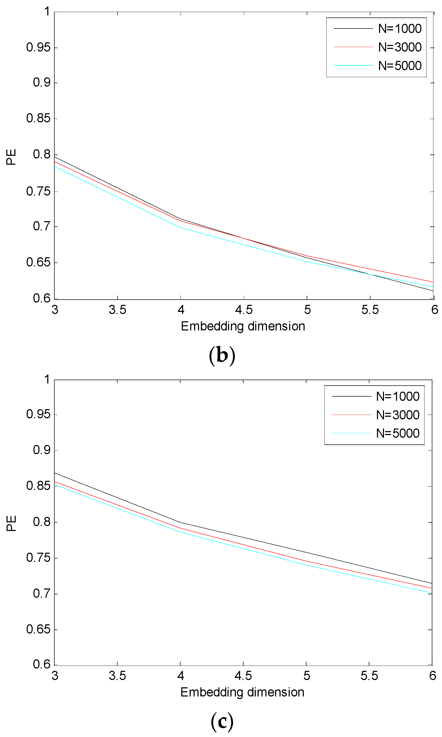
3.1. The Choice of Permutation Entropy Parameters

There are three parameters that need to be considered and set during the calculation of the PE, namely, the length of time series N, embedding dimension m and time delay λ. Bandt proposed that embedding dimension m could be take from 3 to 7 [24], if m is 1 or 2, the reconstructed sequence contains too few states, so the algorithm loses its meaning and validity, and also cannot detect the dynamic mutation of time series. Instead, if m is too large, it is not appropriate because the time series are averaged by phase space reconstruction, and cannot reflect the subtle changes in the sequence. Time delay λ has little influence on the time series, so this paper makes λ = 1. In this paper, we will mainly discuss two parameters: the data length and the embedding dimension.

When considering the influence of the length of the time series, three types of the SRN signals are used to analyze PEs with different lengths. The samples are normalized to get the time-domain waveform of three types of SRN signals shown in Figure 1. The sampling frequency is 44.1 kHz, the data length (respectively 1000, 3000, and 5000) selected from Figure 1.

As illustrated in Figure 2, the PEs of three types of SRN signals decrease as the embedding dimension increases. For the first type of SRN signal, when the embedding dimension is certain, the larger the sequence length N is, the greater the PE is. When m is 6 and N is 5000 or 1000 respectively, the difference of the PEs is nearly 0.1, showing that N = 1000 cannot fully reflect the complexity of the ship signal. For the second and third types of ship signals in the same embedding dimension, different length of series have little influence on the PE. Considering the complexity of the SRN signals, this paper selects N = 5000.

When the series length N is 5000, the influence of the embedding dimension m is studied as a parameter of the PE. The trend of the PEs for the three types of SRN signals can be seen in Figure 3, in agreement with Figure 1, the PEs decrease as the embedding dimension increases. If m is certain, there are some differences in the PEs and the differences are smallest when m is 3. Therefore, we select four as the embedding dimension, which is more discriminating and has a low computational cost.

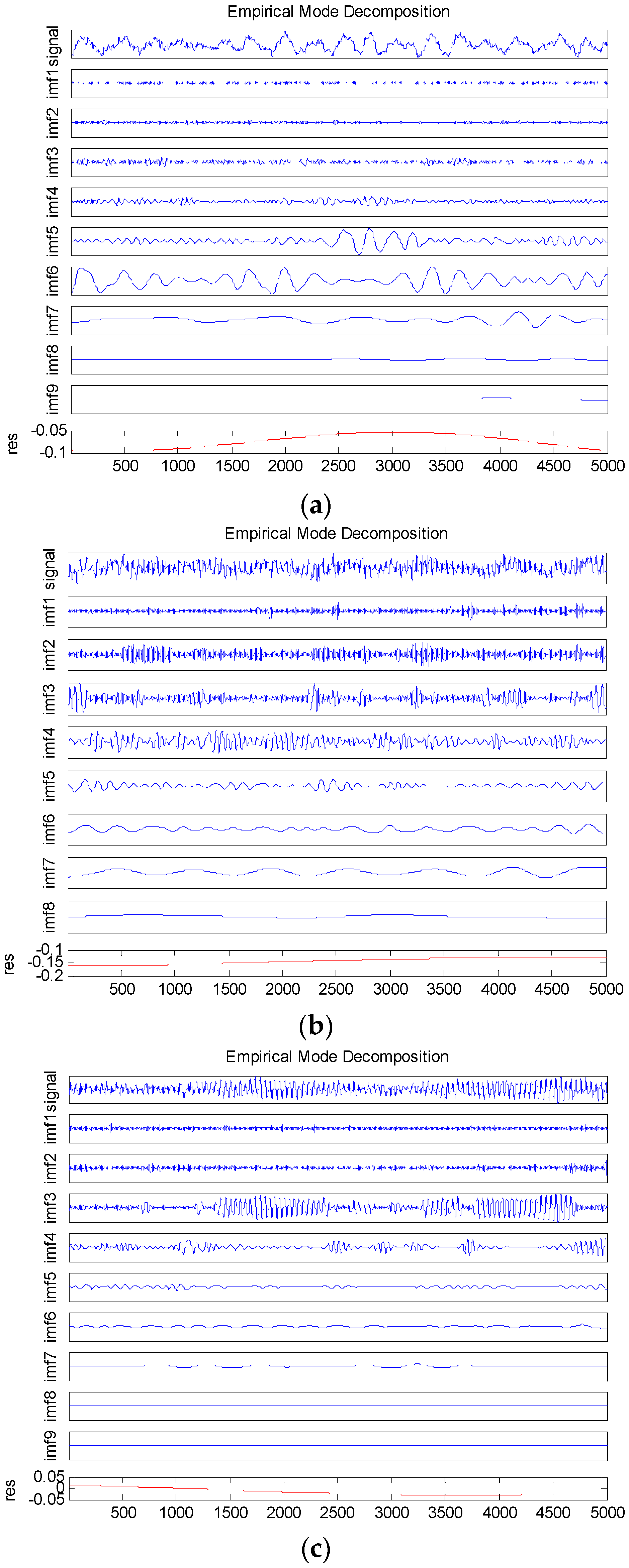
3.2. The Empirical Mode Decomposition of the Ship-Radiated Noise

Three types of SRN signals are analyzed by EMD with a sampling rate of 44.1 kHz and data length of 5000. 100 samples of each type are recorded. Firstly, take Figure 1 with the full 5000 sampling points as the new sample. Then the samples after normalization are decomposed into IMFs (shown in Figure 4), in which the abscissa is the number of sampling point and the ordinate represents the normalized amplitude.

As can be seen in Figure 4, the SRN signals are orderly decomposed into a set of IMFs from high frequency to low frequency with EMD. The first IMFs represent the shortest oscillation period, typically a noise component or the high frequency components. The numbers of the IMFs of each type of SRN signals are not the same. Depending on the oscillatory modes of the signals, the more oscillatory the signal modes are, the more IMFs there are. There are always one or two IMFs with amplitudes that are obviously higher than others. Usually, these are the main energy components that can reflect the most significant characteristic of the SRN signals.

3.3. The PE of Each IMF

Three types of SRN signals are transformed into IMFs after EMD. Figure 5 shows the PEs of the IMFs. The abscissa is the first to eighth IMF of each type and the ordinate indicates the PEs of the IMFs. As can be seen from Figure 5, the PEs of the IMFs decrease as the order of the IMFs increase, indicating that the higher the order of the IMF, the less complexity. The difference between the PEs in the same level of IMF1 and IMF2 are more obvious than other IMFs, but the difference is small. Their main frequency components are found to be higher than 10,000 Hz after the Fourier Transformation, regarding them as noise IMFs. The PEs of IMF3 to IMF8 at the same level is very similar for three types SRN signals, especially the IMFs of high order. The above analysis shows that the PEs of the same level of IMFs have no obvious difference for the three types of SRN signals.

Since the difference of the PEs of the same level IMFs is small, the IMFs are rearranged according to their energy order. Suppose the m-th IMF decomposed from the original data has N sample points and the instantaneous amplitude of the n-th sampling point is b_mn, then its instantaneous intensity is:

Q_mn = b²_mn

(15)

The average intensity of the m-th IMF is:

$$\widehat{B}m=\frac{{\displaystyle \sum _{n=1}^{N}Qmn}}{N}$$

(16)

The average intensity of each level IMFs is determined according to formulas (15) and (16). Figure 6 shows the PEs of the IMFs arranged according to energy descending order. The abscissa is the six IMFs ordered according to the energy from higher to lower without the noise IMFs, whereas the ordinate represents the PE of the six IMFs. As seen in Figure 6, there is no obvious regulation between the IMFs and their PEs. The differences of the PEs between the first IMFs of the three types of SRN signals are quite obvious. However, for the PEs of other IMFs, there are at least two PEs from different types of SRN signals are similar. The above analysis shows that the PEs of the first level IMFs have a great difference than the others at the same level.

4. Feature Extraction of SRN Signal

4.1. Feature Extraction Based on the PE of the IMF with the Highest Energy

By analyzing the PEs of each level IMFs for the three types of SRN signals, we found that the PEs of the first IMFs with higher energy in the IMFs are much different. This paper chooses the IMFs with the highest energy representing main features of the SRN signals to calculate their PE in order to judge their separability.

If the original data is divided into a total of M IMFs, the IMF with the highest average intensity is defined as the EIMF, namely:

$$\widehat{B}\max =\max ( \widehat{B}1, \widehat{B}2,... \widehat{B}M)$$

(17)

$\widehat{B}1$ is the average intensity of the first IMF with EMD. $\widehat{B}2$ and $\widehat{B}M$ are the same with $\widehat{B}1$. $\widehat{B}\max$ is the average intensity of EIMF and it can characterize the main features of the signals. The EIMFs of three types of SRN signals are determined according to formulas (15)–(17), and the PEs of EIMFs for each type of SRN signals are shown in

Table 1. The PEs of the EIMFs for three types of SRN signals.

	First Type	Second Type	Third Type
EIMF (level)	6	4	3
PE of EIMF	0.2528	0.3310	0.4054

. As can be seen from Table 1, the EIMFs of the three types are distributed in different levels, and the PEs of EIMFs are certainly different.

4.2. Feature Extraction Based on MPE

For different types of SRN signals, even the time series of the same ocean, their complexity is different. In order to better describe the change quantitatively, we introduce MPE theory. The MPE can describe the degree of complexity of the time series in different scale.

Figure 7 is the MPEs of three types of SRN signals, where the time sequence length N is 5000, embedding dimension m is 4 and time delay λ is 1, the abscissa is the time scale, and the ordinate is the MPE of SRN signal. It is found that the MPEs of the first type are fluctuated around a fairly stable value as the order of time scale increases, and as for the MPEs of the second and third type, the MPEs are first increasing and then stable with the increase of time scales. They reflect the differences of the three types of SRN signals in different scales. There are some differences for the three types of SRN signals in different time scales, and they are relatively large in the time scales 1 and 17. The MPE is the PE when the time scale is 1.

Table 2. The MPEs for three types of SRN singles (each type includes one sample).

	First Type	Second Type	Third Type
MPE (scale = 1)	0.8837	0.7105	0.7852
MPE (scale = 17)	0.8562	0.9717	0.9123

shows the MPEs for three types of SRN signals when the time scales are 1 and 17. It is found that there are some differences in the PEs of the three types and the MPEs when the scale is 17, but the difference is not obvious, so their separability needs further analysis.

4.3. Feature Extraction Based on Energy Difference

EEMD method is used in reference [15] to extract the feature of SRN signals, among which, a range of 100~1000 Hz is regarded as the low frequency band of SRN and a range of 1000~10,000 Hz is considered the high frequency band, and the energy difference between high frequency and low frequency is defined as the energy difference of SRN signal. For the convenience of comparison, this article uses the energy difference between high frequency and low frequency with EMD as a characteristic parameter, and the concrete calculating steps are as follows.

After signal $x(t)$ is decomposed with EMD, perform Hilbert transform on each IMF $c(t)$:

$$\widehat{c}(t)=\frac{1}{\pi }{\displaystyle \underset{-\infty }{\overset{\infty }{\int }}\frac{c(\tau )}{t-\tau }}\mathrm{d}\tau$$

(18)

its analytic signal can be expressed as

$$z(t)=c(t)+j\widehat{c}(t)=\lambda (t)\exp [j\theta (t)]$$

(19)

wherein, the instantaneous amplitude is $\lambda (t)=\sqrt{c^2(t)+{\widehat{c}}^2(t)}$, instantaneous phase is $\theta (t)=\arctan (\widehat{c}(t)/c(t))$, and instantaneous frequency is

$$f(t)=\frac{1}{2\mathsf{\pi }}\frac{\mathrm{d}\mathsf{\theta }(t)}{\mathrm{d}t}$$

(20)

The sums of high frequency energy and low frequency energy of different IMFs are calculated respectively by formula (15), and the energy difference is equal to the sum of high frequency energy minus the sum of low frequency energy.

Table 3. The energy difference between the high and low frequency (each type includes one sample).

	First Type	Second Type	Third Type
Energy difference (db)	−12.013	−2.4347	−1.5990

shows the energy difference between high and low frequency for the three types of SRN signals. By comparison, it is found that the first type of SRN signals is easier to distinguish than the other two types, while there is a certain difference between the second and third types of SRN signals.

4.4. Comparison of Feature Extraction Methods

To verify whether the difference is universal for the PE of EIMF, energy difference between high frequency and low frequency, PE and MPE as feature parameters for the three types of SRN signals, 50 out 100 samples for each type of SRN signals are randomly selected to calculate the above four feature parameters respectively. In Figure 8, the abscissa is the number of samples, the ordinate represents the PE of EIMFs. Figure 8 reflects the complexity of the EIMFs, showing that the PEs of EIMFs fluctuate within a certain range, with its value at the same level, but there is a significant difference among the PEs of EIMFs for different types of SRN signals.

Figure 9 is the distribution of the PEs for three types of SRN signals, wherein the PEs for the first type of SRN signals are the biggest, and it is more complex than that of the other two. The overall PE of the third type is a little bit higher than that of the second, but the PEs of a few samples are obviously lower than that of the second. Figure 10 shows the MPE when the time scale of the three types is 17. Different from Figure 9, the order of PE for three types of SRN signals has obviously changed, indicating that the three types of SRN signals show different complexity in different time scales. On the whole, Figure 10 shows that the MPEs of the first type of SRN signals are the lowest, the MPEs of the second are the highest, but a few MPEs of third are the similar to the other two when the time scale is 17. It is hard to distinguish the three types of SRN signals by MPE. Figure 11 is the distribution of the energy difference between high and low frequency for three types of SRN signals, it has better separability than the PE and MPE as a characteristic parameter.

Table 4. The four feature parameters for three types SRN signals (each type includes fifty samples).

	First Type	Second Type	Third Type
The average value of PE of EIMF	0.2524	0.3458	0.4287
The range of PE of EIMF	0.2473~0.2612	0.3325~0.3641	0.3825~0.4526
The average value of PE	0.8825	0.7164	0.7482
The range of PE	0.8673~0.8934	0.6926~0.7458	0.7129~0.7912
The average value of MPE (scale = 17)	0.8452	0.9758	0.9137
The range of MPE (scale = 17)	0.7912~0.9034	0.9553~0.9876	0.8457~0.9625
The average value of energy difference (db)	−13.9462~−11.6412	−4.3344~−1.7516	−1.9847~−0.8835
The range of energy difference (db)	−12.6240	−2.9339	−1.4713

further shows the range and average value for the four feature parameters. There is significant difference in the average value of the PE of EIMF and no overlap in their fluctuation range. PE as the feature parameter can only distinguish the first type of SRN signals, the average values are similar and their fluctuation range is largely overlapped for the other two, which cannot distinguish the three types of SRN signals. There are some differences in the average of the MPE when the time scale is 17 and their fluctuation range are partially overlapped, which means poor separability. However, the average value of the energy difference is obviously different and their fluctuation range is slightly overlapped. The above results shows that, compared to the other three feature parameters, the PE of the EIMF can better distinguish the three types of SRN signals.

5. Conclusions

Aiming at feature extraction of SRN signals, a new approach that integrates the EMD with the PE is proposed in this paper, which can distinguish different types of SRN signals well. The first step is to choose the appropriate parameters of PE based on PE theory, then the EMD is used as the pretreatment to decompose SRN signals into a set of IMFs, and the PEs of the IMFs at all levels are calculated. Simulation results show the PEs of the IMFs for the three types of SRN signals decrease obviously with EMD order, but the PEs of the same level IMFs is similar. In order to distinguish the three types of SRN signals, the IMFs are rearranged according to energy descending order, and simulation results show the first PEs of the IMFs with greater energy are significant different from that of the other IMFs.

Based on the above conclusions, the PE of EIMF for three types of SRN signals is selected as a new feature parameter. Compare it with the energy difference with EMD, the PE and the MPE of the SRN signals, simulation results show the same type of SRN signals has similar feature parameter, but variation is in different levels between different types of SRN signals. The energy difference with EMD is superior to the PE and the MPE without EMD as a feature parameter, so EMD method is beneficial for the feature extraction of the SRN signals. Furthermore, the PE of EIMF, which combines of both EMD and PE, can fully reflect the complexity of the target features, and has better separability than the energy difference as a feature parameter. Consequently, the PE of EIMF has a certain reference value for further underwater target detection and identification.

References

1. Wang, S.; Zeng, X. Robust underwater noise targets classification using auditory inspired time-frequency analysis. Appl. Acoust. 2014, 78, 68–76. [Google Scholar] [CrossRef]
2. Urick, R.J. Principles of Underwater Sound, 3rd ed.; McGraw-Hill: New York, NY, USA, 1983. [Google Scholar]
3. Liu, S.; Zhang, X.; Niu, Y.; Wang, P. Feature extraction and classification experiment of underwater acoustic signals based on energy spectrum of IMF’s. CEA 2014, 3, 203–206. [Google Scholar]
4. Huang, N.E.; Shen, Z.; Long, S.R.; Wu, M.C.; Shih, H.H.; Zheng, Q.; Yen, N.C.; Tung, C.C.; Liu, H.H. The empirical mode decomposition and the Hilbert spectrum for nonlinear and non-stationary time series analysis. Proc. R. Soc. Lond. 1998, 454, 903–995. [Google Scholar] [CrossRef]
5. Wu, Z.; Huang, N.E. A study of the characteristics of white noise using the empirical mode decomposition method. Proc. R. Soc. Lond. 2004, 460, 1597–1611. [Google Scholar] [CrossRef]
6. Hsieh, N.K.; Lin, W.Y.; Young, H.T. High-Speed Spindle Fault Diagnosis with the Empirical Mode Decomposition and Multiscale Entropy Method. Entropy 2015, 17, 2170–2183. [Google Scholar] [CrossRef]
7. Zhang, Z.; Shi, X.; Chen, Z.; Tang, B. Fault Feature Extraction of Rolling Element Bearing Based on Improved EMD and Sliding Kurtosis Algorithm. J. Vib. Shock 2012, 31, 80–83. [Google Scholar]
8. Wei, Q.; Liu, Q.; Fan, S.-Z.; Lu, C.-W.; Lin, T.-Y.; Abbod, M.F.; Shieh, J.-S. Analysis of EEG via Multivariate Empirical Mode Decomposition for Depth of Anesthesia Based on Sample Entropy. Entropy 2013, 15, 3458–3470. [Google Scholar] [CrossRef]
9. Sharma, R.; Pachori, R.B.; Acharya, U.R. Application of entropy measures on intrinsic mode functions for automated identification of focal electroencephalogram signals. Entropy 2015, 17, 669–691. [Google Scholar] [CrossRef]
10. Shih, M.-T.; Doctor, F.; Fan, S.-Z.; Jen, K.-K.; Shieh, J.-S. Instantaneous 3D EEG Signal Analysis Based on Empirical Mode Decomposition and the Hilbert–Huang Transform Applied to Depth of Anaesthesia. Entropy 2015, 17, 928–949. [Google Scholar] [CrossRef]
11. Hou, W.; Feng, G.-L.; Dong, W.-J. A technique for distinguishing dynamical species in the temperature time series of North China. Acta Phys. Sin. 2006, 55, 2663–2668. [Google Scholar]
12. Xue, C.; Hou, W.; Zhao, J.; Wang, S. The application of ensemble empirical mode decomposition method in multiscale analysis of region precipitation and its response to the climate change. Acta Phys. Sin. 2013, 62, 109203. [Google Scholar]
13. Zhang, Z.; Liu, C.; Liu, B. Ship noise spectrum analysis based on HHT. In Proceedings of the 2010 IEEE 10th International Conference on Signal Processing (ICSP), Beijing, China, 24–28 October 2010; pp. 2411–2414.
14. Yang, L. A empirical mode decomposition approach to feature extraction of ship-radiated noise. In Proceedings of the 4th IEEE Conference on Industrial Electronics and Applications, Xi’an, China, 25–27 May 2009; pp. 3682–3686.
15. Yang, H.; Li, Y.; Li, G. Energy analysis of ship-radiated noise based on ensemble empirical mode decomposition. J. Vib. Shock 2015, 34, 55–59. [Google Scholar]
16. Zanin, M.; Zunino, L.; Rosso, O.A.; Papo, D. Permutation Entropy and Its Main Biomedical and Econophysics Applications: A Review. Entropy 2012, 14, 1553–1577. [Google Scholar] [CrossRef]
17. Ravelo-García, A.G.; Navarro-Mesa, J.L.; Casanova-Blancas, U.; Martin-Gonzalez, S.; Quintana-Morales, P.; Guerra-Moreno, I.; Canino-Rodríguez, J.M.; Hernández-Pérez, E. Application of the Permutation Entropy over the Heart Rate Variability for the Improvement of Electrocardiogram-based Sleep Breathing Pause Detection. Entropy 2015, 17, 914–927. [Google Scholar] [CrossRef]
18. Shi, Z.; Song, W.; Taheri, S. Improved LMD, Permutation Entropy and Optimized K-Means to Fault Diagnosis for Roller Bearings. Entropy 2016, 18, 70. [Google Scholar] [CrossRef]
19. Yan, R.; Liu, Y.; Gao, R.X. Permutation entropy: A nonlinear statistical measure for status characterization of rotary machines. Mech. Syst. Signal Process. 2012, 29, 474–484. [Google Scholar] [CrossRef]
20. Zhao, L.-Y.; Wang, L.; Yan, R.-Q. Rolling Bearing Fault Diagnosis Based on Wavelet Packet Decomposition and Multi-Scale Permutation Entropy. Entropy 2015, 17, 6447–6461. [Google Scholar] [CrossRef]
21. Qin, N.; Jiang, P.; Sun, Y.; Jin, W. Fault Diagnosis of High Speed Train Bogie Based on EEMD and Permutation Entropy. J. Vib. Meas. Diagn. 2015, 35, 885–891. [Google Scholar]
22. Wu, T.-Y.; Yu, C.-L.; Liu, D.-C. On Multi-Scale Entropy Analysis of Order-Tracking Measurement for Bearing Fault Diagnosis under Variable Speed. Entropy 2016, 18, 292. [Google Scholar] [CrossRef]
23. Aziz, W.; Arif, M. Multiscale Permutation Entropy of Physiological Time Series. In Proceedings of the Pakistan Section Multitopic Conference INMIC, Karachi, Pakistan, 23–25 December 2005.
24. Bandt, C.; Pompe, B. Permutation entropy: A natural complexity measure for time series. Phys. Rev. Lett. 2002, 88, 174102. [Google Scholar] [CrossRef] [PubMed]
Figure 1. The time-domain waveform for three types of SRN signals. (a) The first type of SRN signal; (b) The second type of SRN signal; (c) The third type of SRN signal.
Entropy 18 00393 g001aEntropy 18 00393 g001b
Figure 2. The PEs for three types of SRN signals with different embedding dimension and sequence length. (a) The first type of SRN signal; (b) The second type of SRN signal; (c) The third type of SRN signal.
Entropy 18 00393 g002aEntropy 18 00393 g002b
Figure 3. The PEs for three types of SRN signals with different embedding dimension.
Entropy 18 00393 g003
Figure 4. The results of EMD for three types of SRN signals. (a) The first type of SRN signal; (b) The second type of SRN signal; (c) The third type of SRN signal.
Entropy 18 00393 g004
Figure 5. The PEs of IMFs for the three types of SRN signals.
Entropy 18 00393 g005
Figure 6. The PEs of the IMFs arranged according to energy descending order.
Entropy 18 00393 g006
Figure 7. The MPEs for three types of SRN signals.
Entropy 18 00393 g007
Figure 8. The PEs of the EIMFs for three types of SNR signals.
Entropy 18 00393 g008
Figure 9. The PE for three types of SNR signals.
Entropy 18 00393 g009
Figure 10. The MPE for three types of SNR signals (scale = 17).
Entropy 18 00393 g010
Figure 11. The energy difference between the high and low frequency for three types of SNR signals.
Entropy 18 00393 g011