1. Introduction
It is known that many physical systems can be described by fractals. Railway networks (RN) are one such type of system. Suburban railway networks of several cities (Paris, Moscow, Rhine conurbation, Seoul, Beijing, and Mexico City) were studied in this respect [
1,
2,
3,
4], but published literature analyses these networks only at the time of writing. The sole exception is [
3], which covers a few decades.
Biological systems with fractal structure include the circulatory and respiratory systems in humans [
5], or the circulation of sap in trees [
6,
7]. Among these, commuting resembles the respiratory system most, where flow takes place in both directions in the same pathway. The knowledge of a system’s fractal structure is important to determine its dynamic behavior, which often turns out to include phenomena of fractional or anomalous diffusion [
8,
9].
This paper studies the Portuguese railway system, for the entire territory located in Europe, and analyzes its evolution over time, since the first line was opened in 1856. Loosely speaking, we study how evenly the RNs spread over the Portuguese territory over one and a half centuries. Our purpose is to study the RN dynamics and to compare what is qualitatively known from history with our quantitative results. For that purpose, we adopt, as mathematical tools, fractal dimension, entropy, and state portrait (SSP). The first tool, as mentioned, has been used for suburban RNs; the last two are, to the best of our knowledge, new for this application. They have, however, been applied in [
10,
11,
12]. The analysis presented is descriptive, as is the case with [
1,
2,
3,
4], and serves to confirm the qualitative history of the RN. It is aimed at an academic study in the area of geography. Once the dynamic behavior of the RN is known, understanding its fractal geometry will be of importance for planning extensions or closures of lines, making the method relevant for a wider audience.
The evolution of the RN was crucial for the economic development of the country, as alternative means of transportation available until the second quarter of the 20th century were clearly inferior: navigable rivers in Portugal are not long and allow access to only a limited part of the territory, and road transport only becomes a serious alternative with the development of efficient internal combustion engines. While limited by geographical reasons (especially by the mountainous orography of the North of Portugal, which anyway also hinders road construction and completely precludes building canals), the RN was faster and cheaper, and allowed an increased regional specialization of the economy [
13]. Even though modern economic growth failed to take hold of Portugal before the end of the Second World War, the social and economic changes induced by the introduction of railway transportation were very significant [
14], and it is therefore relevant to study the evolution of its structure.
The paper is organized as follows.
Section 2 briefly describes the Portuguese railway system.
Section 3 and
Section 4 study the time evolution of the RN by means of fractal geometry and entropy versus time, and SSP of entropy, respectively.
Section 5 discusses the results obtained. Finally,
Section 6 draws the main conclusions, perspectives, and future work, and foresees possible manners of incorporating these results in planning.
2. The Portuguese Railway System
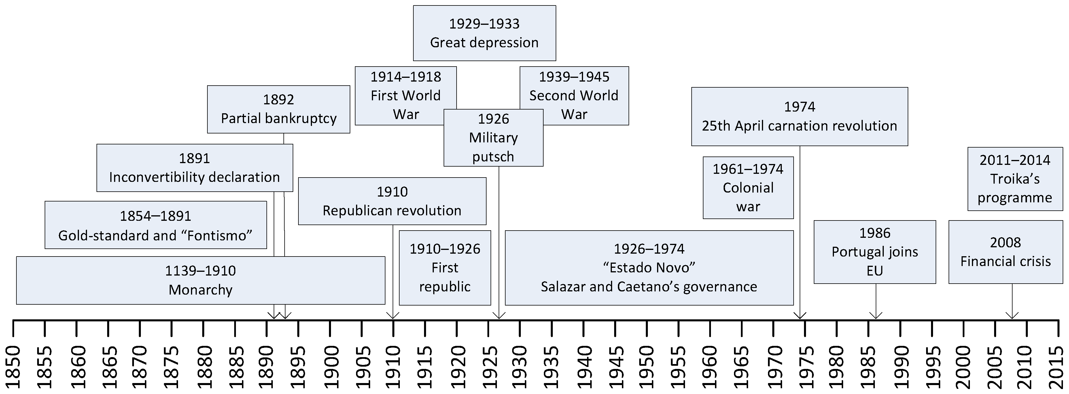
The development of the RN has been closely related to the Portuguese history over the last century and a half.
Figure 1 is a timeline of the main socio-economic events.
The RN began in 1856 when the first stations of a line that would connect Lisbon to Porto and to Madrid, Spain were opened. Lines were built both by public and private initiatives. In fact, the original aim was to link Lisbon to Madrid, with a branch to reach Porto. Shortly thereafter, this plan became a line to connect Lisbon and Porto, and the connection to Spain became secondary. Connections to France and the rest of Europe always had to overcome the difficulty of a change of gauge at the Spanish–French border.
The heyday of the RN was the mid-20th century; the economic and social importance of this means of transportation has since been decreasing, particularly due to an increasing importance of road transportation for both passengers and cargo. Nearly all existing lines are built with Iberian gauges (1668 mm according to present standards). Two lines with meter gauges (1000 mm) still exist; this gauge was typical in secondary lines in the north of Portugal (where the mountainous orography makes a narrower gauge cheaper to build), but these have nearly all been closed. Indeed, many lines with low traffic and no commercial interest ceased operations in 1988–1992, and others in 2008–2012. A few short lines have been built in this period, all of them for cargo, with the exception a suburban connection from Lisbon to its south suburbs on the other side of the Tagus River. Readers interested in a detailed history of the Portuguese railway system may consult [
16,
17].
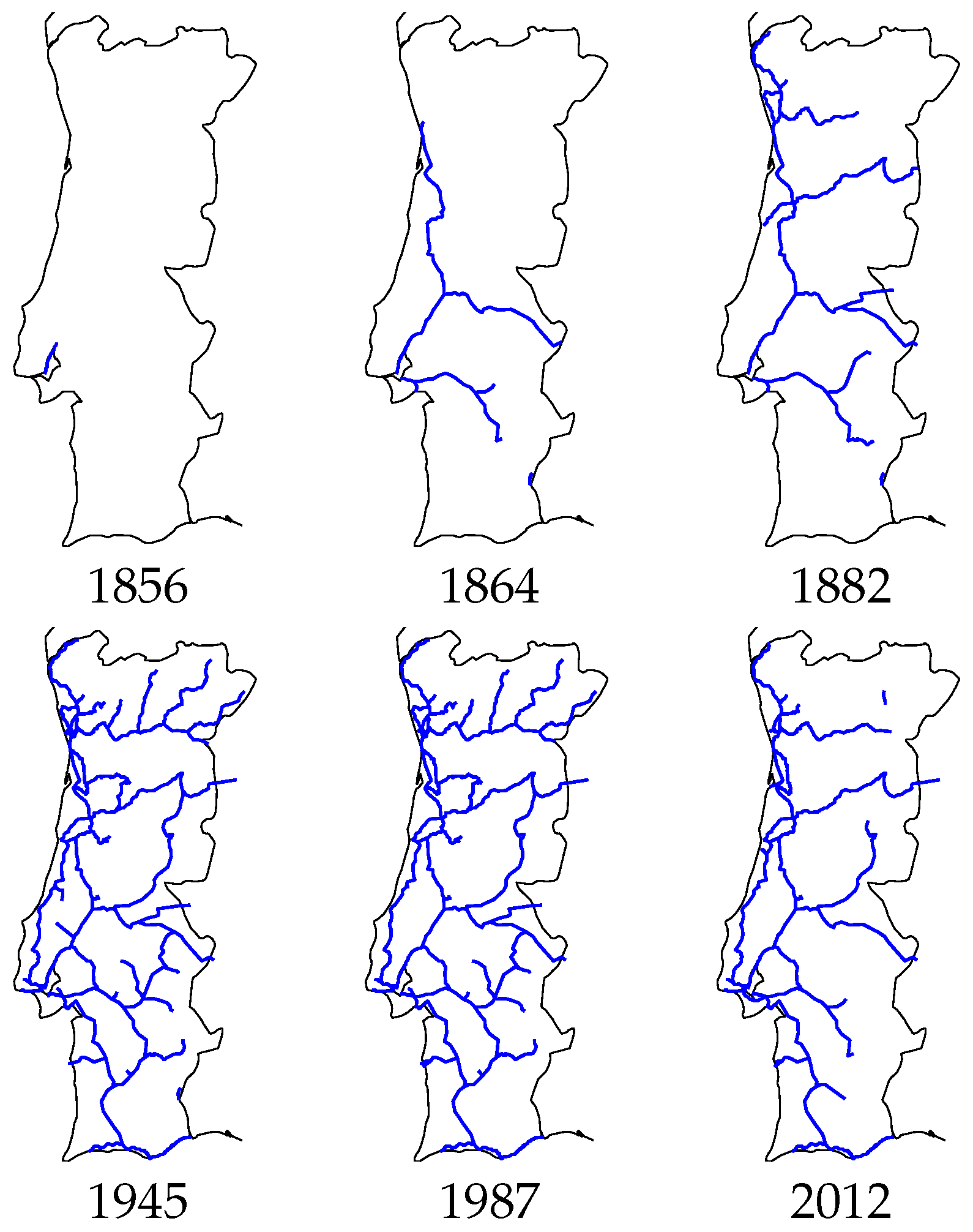
While there is no room to show changes for every single year in which stations opened or closed,
Figure 2 presents several maps, for chosen significant years unevenly spaced in time, from which the evolution of the RN with time is clear. Notice that, for obvious geographical reasons, all lines are on the European continent; no RNs have ever been built in the Azores and Madeira islands (Lines in Portuguese colonies during this period are not only outside the scope of this paper, but also have little interest for our purpose, since no colony ever had a proper network, but, at most, only unconnected lines).
This paper concentrates on the railway system proper, not taking into account underground networks or trams; these are not connected to the railway system except for passenger interfaces, while Iberian and meter gauge lines were connected for both passenger and cargo. For each year, those lines that were operated publicly or privately are considered; therefore, lines under construction or lines still available, but without traffic, are disregarded. The RN is considered as a graph, where each station is a node. The geographical coordinates of train stations and the years when they were open and closed to service were found conjugating information in [
17,
18,
19]. For international lines, the first station in Spanish territory was included. This graph concerns the geography of the line only, so differences in traffic flow are not taken into account, which lines are double-track, which are electrified, the maximum speeds attainable, extant signaling technology, or any other variable related to the quality of the line or the intensity of its use.
3. Fractal Dimension of the Portuguese Railway Network
A fractal is a geometrical object displaying a pattern repeated at different scales. The pattern may occur repeated exactly or approximately. While mathematical objects can repeat a pattern at all scales, infinitely large and infinitely small, actual plants reveal a fractal nature only within a range of scales. An RN is a good example, since scales larger than a continent or smaller than the gauge have no physical sense. The fractal dimension is a measure of how much the fractal fills the space as it is magnified from larger to smaller scales, for which there are several definitions, that in general do not coincide [
20,
21,
22]. The definition more often found in practice is the box-counting fractal dimension, due to its easy numerical implementation. The algorithm can be described as follows:
Repeat:
- -
cover the fractal object S with a grid consisting of squares (the boxes) with size ,
- -
find the number of boxes that include part of the fractal ,
- -
decrease ϵ.
The fractal dimension
is the slope of the log-log plot of
vs.
ϵ, i.e.,
In other words, the fractal dimension is estimated as the exponent of a power law:
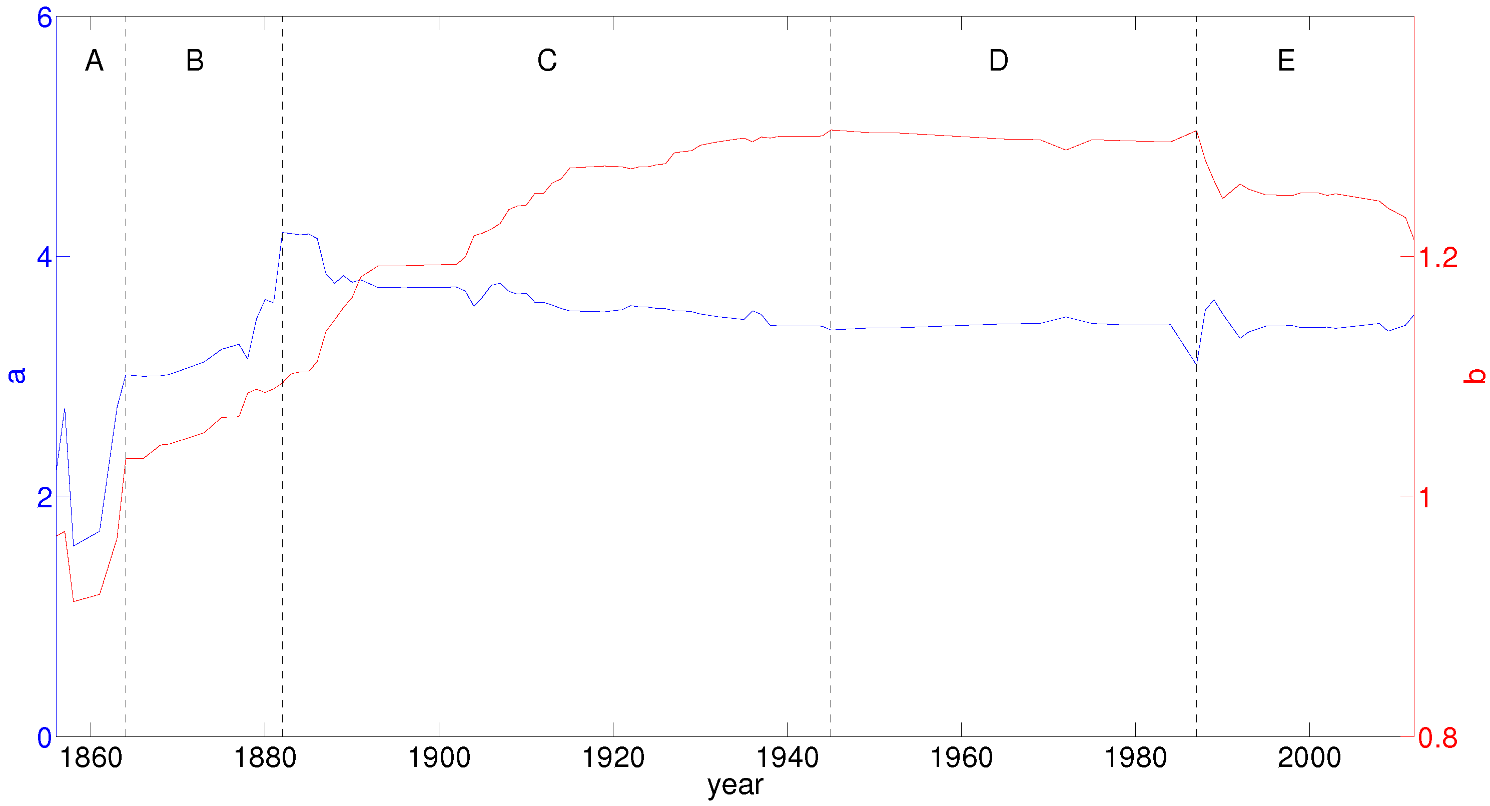
Here, is related to the length between bifurcations of the RN.
Figure 3 depicts the evolution of parameters
a and
b with time.
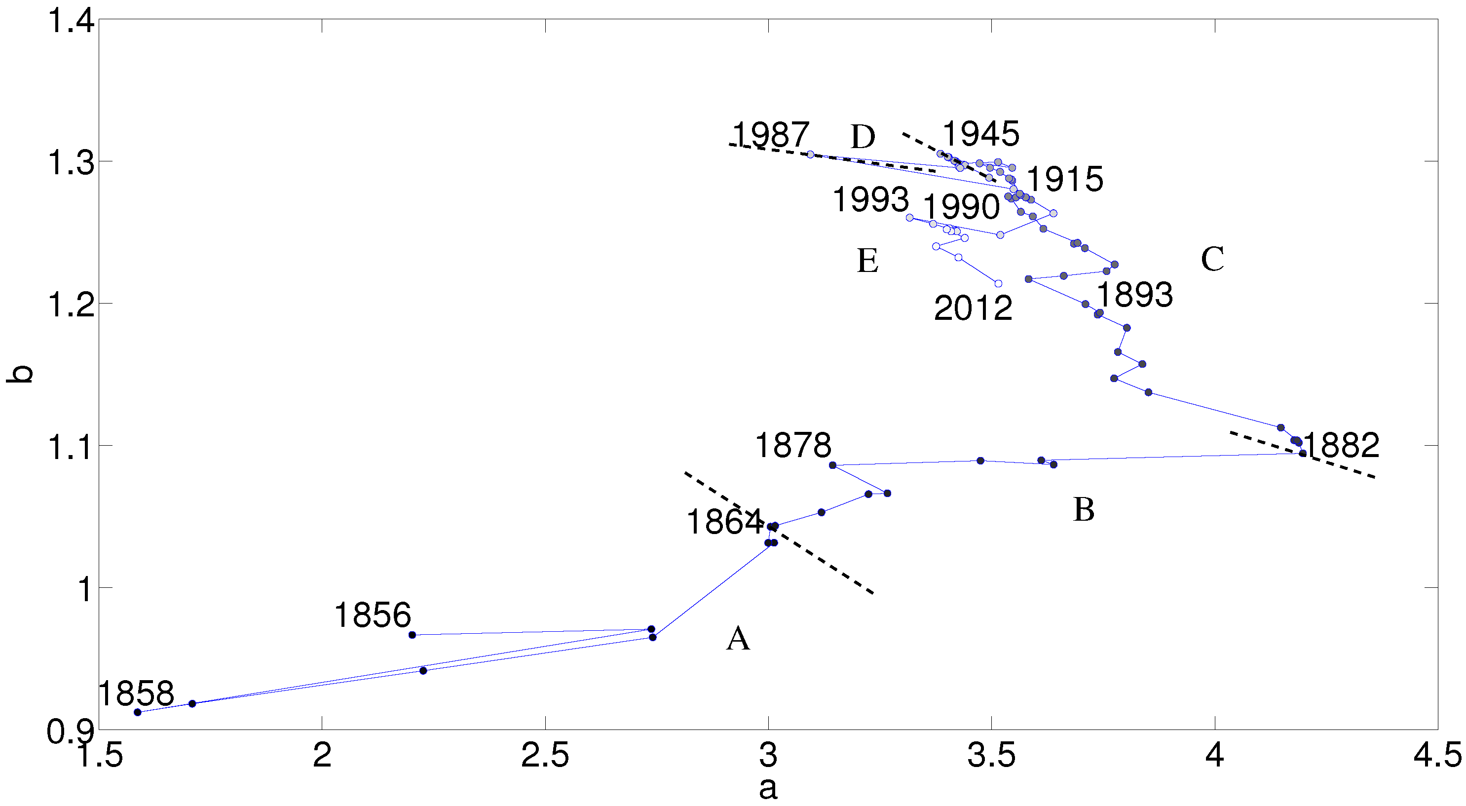
Figure 4 shows how they are related to each other. From these figures, it is seen that results can be conveniently divided into five periods, discussed in
Section 6.
4. Entropy and SSP Analysis of the Portuguese Railway Network
The availability of the RN was never uniform in the Portuguese territory. In this section, the uniformity, or lack thereof, of the distribution of train lines throughout the country is assessed by means of entropy and SSP.
4.1. Entropy of the Railway Network
Entropy plays an important role in the area of information theory and statistical mechanics. In the last decades, generalizations of the classic Boltzmann–Gibbs–Shannon formulation have been proposed, namely to explain the statistical nature of many complex systems that follow asymptotic power–law statistical distributions. These generalizations are often expressed in terms of a set of parameters, and, usually, do not obey the fourth Khinchin axiom [
23]. Examples are the Tsallis [
24], Rényi [
25], Ubriaco [
26], Kaniadakis [
27,
28], Sharma–Mittal [
29,
30], and Gamma [
31,
32] entropies, among others [
33,
34,
35,
36,
37,
38,
39]. For certain particular values of the parameters, the classical entropic formulations are recovered.
The Boltzmann–Gibbs–Shannon entropy is given by:
and represents the expected value of the information content,
, of an event with probability of occurrence
, where
.
The Tsallis,
, and Rényi,
, formulations are parametric entropies, given by:
where
and
. In the limit
, the Boltzmann–Gibbs–Shannon entropy is obtained.
Fractional calculus (FC) deals with the generalization of integrals and derivatives to an arbitrary real or complex order [
40,
41,
42,
43,
44,
45]. FC goes back to the beginning of the theory of calculus, but it was just in the last decades that FC was found to play an important role in modeling many physical phenomena, and emerged as an important tool in the area of dynamical systems with complex behavior. FC is able to capture long range phenomena, often overlooked by standard differential equations, being an interesting tool for analyzing phenomena that occur in many dynamical systems [
5,
7,
46,
47,
48,
49,
50,
51,
52,
53,
54,
55,
56,
56].
ionescu:2013
By adopting the tools of FC, the concepts of information content and entropy were recently revisited, leading to the information content and entropy of fractional order
[
57,
58]:
where
is the derivative of order
α and
and
represent the gamma and digamma functions, respectively.
This fractional (or generalized) entropy (Equation (
7)) does not obey some of the Khinchin axioms, except for
[
57]. In this case, it leads to the classical Boltzmann–Gibbs–Shannon entropy (Equation (
3)).
For calculating the entropy of the RN, the probabilities are estimated according to the following procedure. First, the train lines are interpreted as a succession of evenly spaced points, with a step of approximately 1 km (chosen so that a lower value does not significantly change results), interpolated in-between the stations. Second, a rectangular grid with a step (chosen like the step between points) and N divisions is superimposed over the RN. Finally, the probabilities are computed by means of , where is the number of points in each division of the grid i, and n is the total number of points in all N divisions.
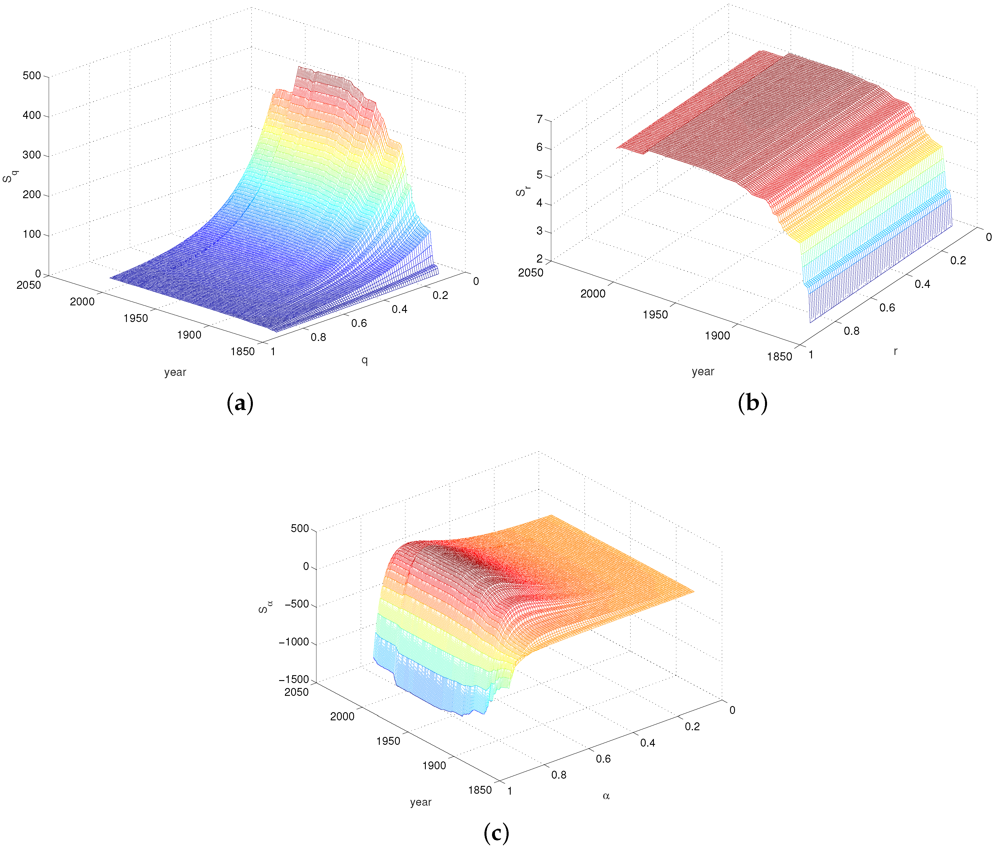
Figure 5 depicts the variation of the Tsallis, Rényi and fractional entropies versus time and the parameters
, respectively. The fractional entropy,
, has a maximum for
. The Tsallis and Rényi entropies are both monotonic in the parameters, and
varies little with
r. Furthermore,
is more sensitive to changes in its parameter
α, and leads to better discrimination between entropy values. The fractional entropy was also compared with other entropic formulations [
59] leading to similar conclusions.
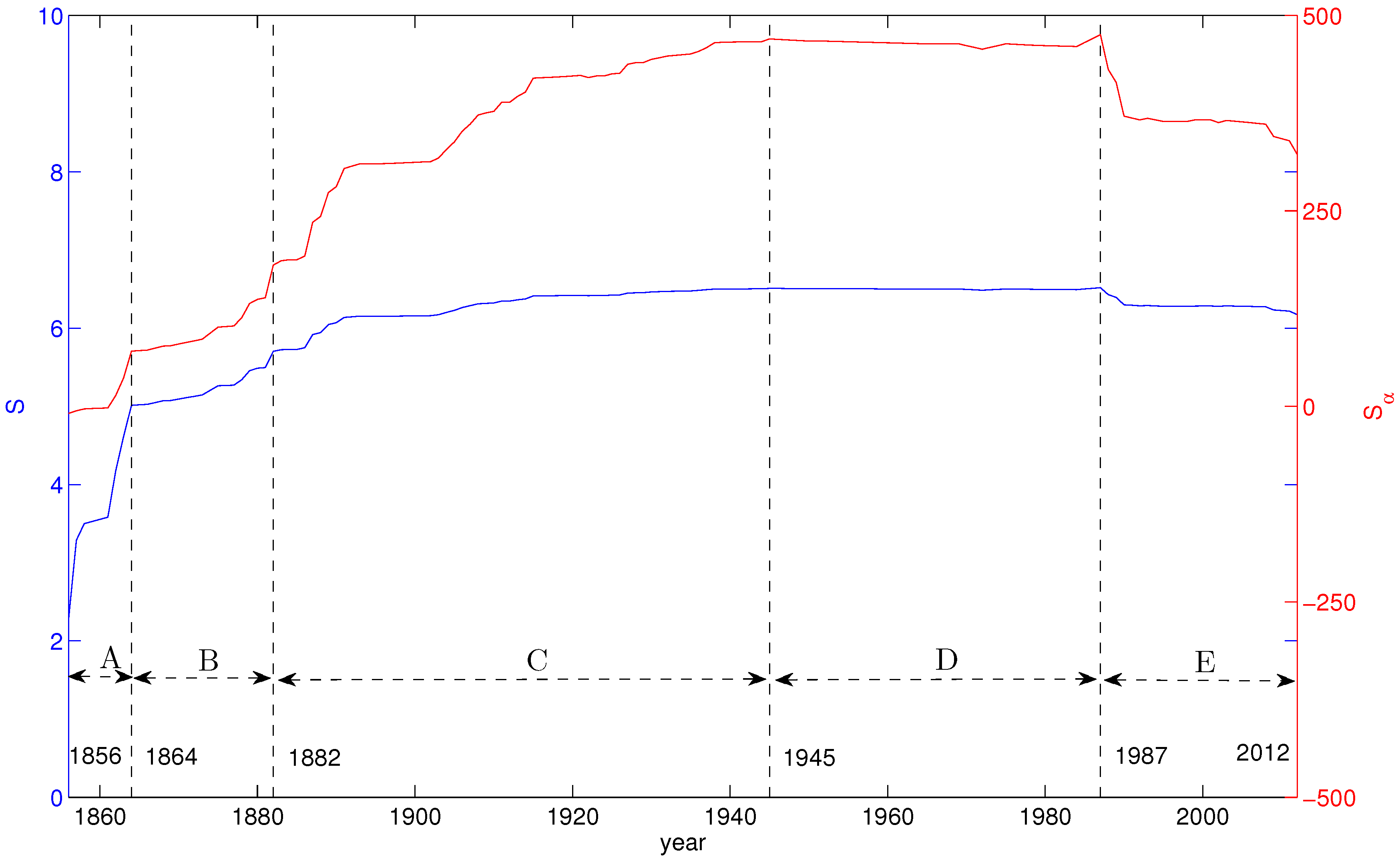
Figure 6 depicts the time evolution of the Boltzmann–Gibbs–Shannon,
S, and fractional,
(
), entropies for the period 1856–2012. We verify that
is able to “amplify” details improving the resolution of the entropy charts.
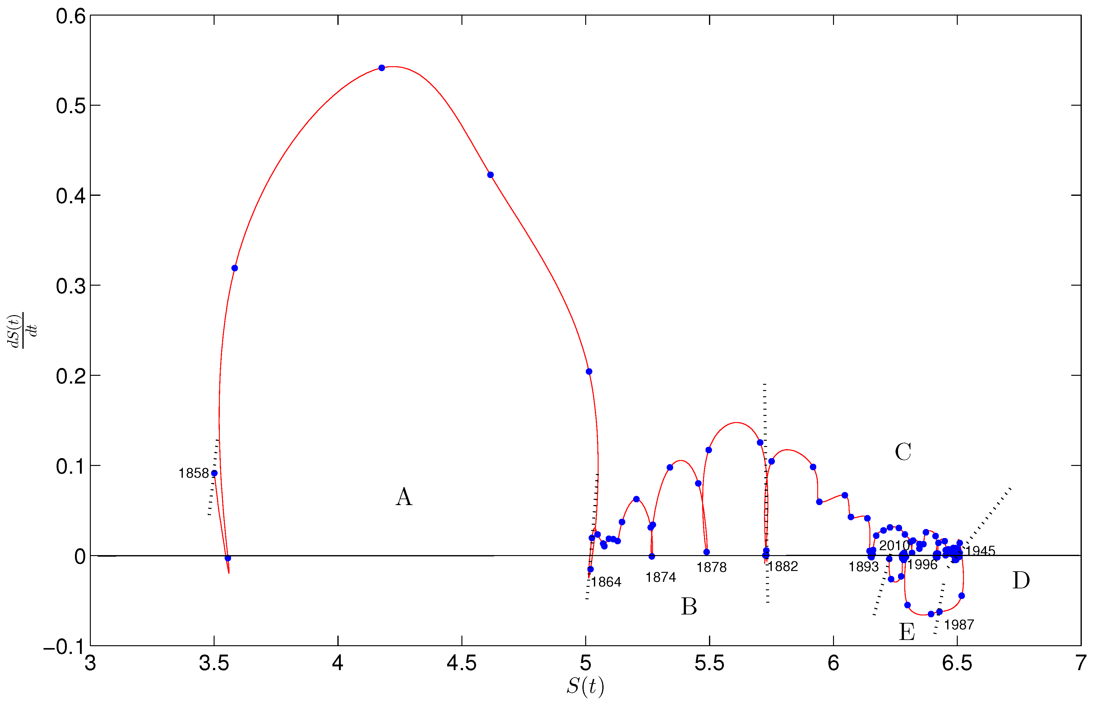
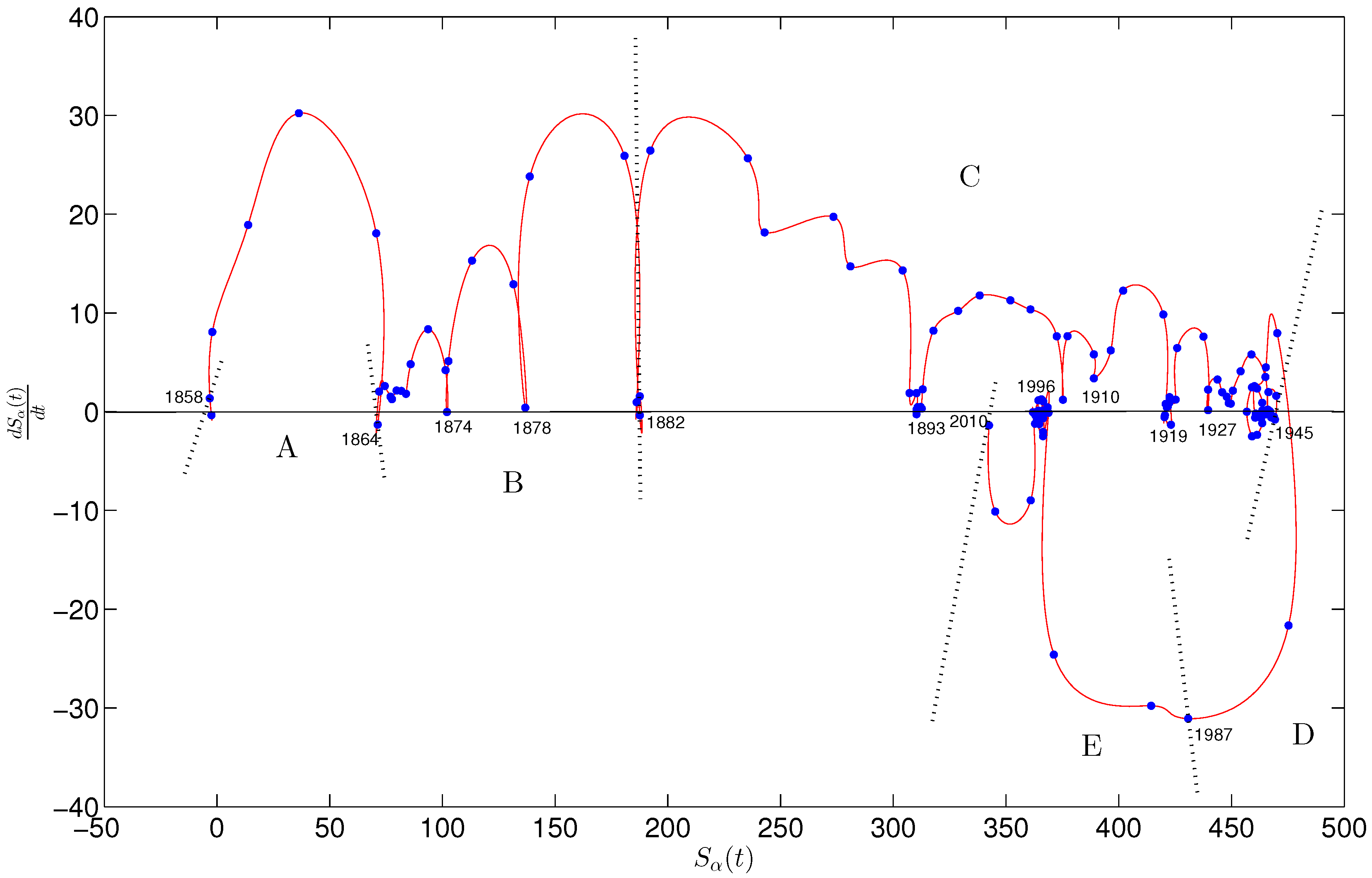
4.2. The SSP of the Railway Network Entropy
For a
k-dimensional dynamical system, the state space consists of the set of all possible states, each one corresponding to a unique point. As time evolves, sequences of points describing trajectories are obtained. The set of trajectories is the SSP. For first, second, and third-order systems, the SSP can be depicted and the system behavior can be inferred from the corresponding graphical representation [
60,
61].
For constructing the SSP, phase variables are adopted, namely the time evolution of the entropy in the period 1856–2012 and its time derivatives. As the order of the system differential model is unknown, successive increasing values of k were tested, and it was found that the two-dimensional space is a good compromise between assertiveness and feasibility of the SSP representation.
Noise may occur in the numerical calculation of the time derivatives. Therefore, the following algorithm [
62] that avoids saturating the resulting signals is considered:
where
h denotes the sampling period.
It must be noted that (Equation (
8)) requires two additional points at the left and the right. Therefore, the SSP turns out to be limited to the period 1858–2010. Several numerical experiments demonstrated that these formulae produce good results for the signals under analysis.
Figure 7 and
Figure 8 show the two-dimensional SSP representations, with
year, for entropies
S and
(
), respectively. As can be seen, the fractional entropy leads to a SSP representation where details can be identified easily, since the chart has more resolution. On the contrary, the main loop corresponding to years 1958–1864 saturates the classic SSP chart, making for difficult the observation of small cycles.
The results obtained from fractal dimension and entropy plus SSP analysis are consistent with each other, and are discussed in the next section.
5. Discussion
The five periods of the Portuguese RN that can be found from the results above are as follows:
Period A: 1856–1864. The first train line opened in 1856, but there was not yet a proper RN during the first eight years. Therefore, this initial period should be overlooked. Spurious oscillations can be seen in the variations of the fractal parameters a and b. The entropy grows fast, as lines start reaching all regions; this corresponds to the biggest loop in the SSP plane of S and .
Period B: 1864–1882. There is growth of the fractal dimension b of the network, but, more important still, there is an increase of the length of the average connection between two bifurcations of the network, as parameter a shows. Entropy grows again increasingly, even if not as much as before. In other words, more than interconnections, longer lines were being built.
Period C: 1882–1945. The fractal dimension b of the network keeps growing; periods of little increase are indeed those of little growth of the network. However, the inter-connectivity of the RN now increases in such a way that the average length of the connection between two bifurcations decreases. Entropy grows, but at an increasingly lower rate until stagnation occurs. In other words, it is not necessary to travel long before finding some bifurcation.
Period D: 1945–1987. This is a period of stagnation, during which few changes in the network take place.
Period E: 1987–2012. The closing of lines at the end of the 1980s was a big change: parameter b decreases sharply, there is likewise a significant drop in entropy, and the same happens again with the closing of lines in 2008–2012. The average length of the connection between two bifurcations increases as lines are closed, but goes down as new short lines are built, as can be seen from the evolution of a.
All mentioned periods can be easily identified in the SPP chart of the entropy. Therefore, we conclude that the methods presented here lead to identical results.
6. Conclusions
The results discussed in the section above fit well with the short sketch of the evolution of the RN outlined in
Section 2 and found in the references quoted. However, and even though they do reflect the changing role of railway transportation, they do so only partially, since line closures take place well after trains cease to be relevant in a certain region. Many lines are kept open for many years with few trains, few passengers, and few tons of cargo, awaiting a political decision about what to do. Actually, the 1945–1987 period of stagnation is a period when, while the network remains the same, significant changes are actually taking place (e.g., introduction of diesel locomotives, overhead electrification, end of the system of separate company franchises running different lines).
To study these issues quantitatively, future work will include analyzing figures for traffic of both passengers and cargo, as the flow efficiency and the percentage of the usage of the RN will have to play a more quantified role. Once this is done, it might be possible to use changes in fractal dimension and entropy to help plan new branches or minimize the effects of closures. In fact, only an RN with significant values of fractal dimension and entropy will be resilient to unscheduled service interruptions. When capacity is considered, not only new lines and line closures, but also variations in the capacity of existing lines or branches may be studied in this regard. Such results will, of course, have to be integrated with the existent models, and with financial, political or social concerns. However, it is relevant that, though the fractal nature of some suburban RNs has been studied for years, it is not considered in state-of-the-art modelling of passenger flows [
63] or freight flows [
64,
65,
66].
Such developments will be considered in future research, in the image of the biological systems with a fractal nature.
Acknowledgments
The authors thank Nuno Valério and Maria Eugénia Mata for pointing out interesting bibliographical items. This work was partially supported by Fundação para a Ciência e a Tecnologia, through IDMEC under LAETA.
Author Contributions
Duarte Valério, António M. Lopes and José A. Tenreiro Machado conceived, designed and performed the experiments, analyzed the data and wrote the paper. All authors have read and approved the final manuscript.
Conflicts of Interest
The authors declare no conflict of interest.
References
- Benguigui, L.; Daoud, M. Is the suburban railway system a fractal? Geogr. Anal. 1991, 23, 362–368. [Google Scholar] [CrossRef]
- Benguigui, L. The fractal dimension of some railway networks. J. Phys. I 1992, 2, 385–388. [Google Scholar] [CrossRef]
- Kim, K.S.; Benguigui, L.; Marinov, M. The fractal structure of Seoul’s public transportation system. Cities 2003, 20, 31–39. [Google Scholar] [CrossRef]
- Sun, Z. The study of fractal approach to measure urban rail transit network morphology. J. Transp. Syst. Eng. Inf. Technol. 2007, 7, 29–38. [Google Scholar]
- Ionescu, C.M. The Human Respiratory System—An Analysis of the Interplay between Anatomy, Structure, Breathing and Fractal Dynamics; Springer: London, UK, 2013. [Google Scholar]
- Ionescu, C.; Machado, J.A.T. Mechanical properties and impedance model for the branching network of the sapping system in the leaf of Hydrangea Macrophylla. Nonlinear Dyn. 2010, 60, 207–216. [Google Scholar] [CrossRef]
- Lopes, A.M.; Machado, J.A.T. Fractional order models of leaves. J. Vib. Control 2014, 20, 998–1008. [Google Scholar] [CrossRef]
- Park, H.W.; Choe, J.; Kang, J.M. Pressure behavior of transport in fractal porous media using a Fractional Calculus approach. Energy Sources 2000, 22, 881–890. [Google Scholar]
- Magin, R.L. Fractional Calculus in Bioengineering; Begell House: Redding, CT, USA, 2006. [Google Scholar]
- Lopes, A.M.; Machado, J.A.T.; Mata, M.E. Analysis of global terrorism dynamics by means of entropy and state space portrait. Nonlinear Dyn. 2016, 85, 1547–1560. [Google Scholar] [CrossRef]
- Lopes, A.M.; Machado, J.A.T. State Space Analysis of Forest Fires. J. Vib. Control 2016, 22, 2153–2164. [Google Scholar] [CrossRef]
- Lopes, A.M.; Machado, J.A.T. Integer and Fractional Order Entropy Analysis of Earthquake Data-series. Nonlinear Dyn. 2016, 84, 79–90. [Google Scholar] [CrossRef]
- Valério, N.; Mata, M.E. The Concise Economic History of Portugal: A Comprehensive Guide. J. Bus. Hist. 2011, 54, 818–820. [Google Scholar]
- Justino, D. A Formação do Espaço Económico Nacional; Vega Editores: Lisboa, Portugal, 1989. (In Portuguese) [Google Scholar]
- Machado, J.A.T.; Mata, M.E. Multidimensional Scaling Analysis of the Dynamics of a Country Economy. Sci. World J. 2013, 2013, 594587. [Google Scholar]
- Da Silveira, L.E.; Alves, D.; Lima, N.M.; Alcântara, A.; Puig, J. Population and Railways in Portugal, 1801–1930. J. Interdiscip. Hist. 2011, 42, 29–52. [Google Scholar] [CrossRef]
- Valério, N.; Costa, S.D. Acessibilidade das várias regiões de Portugal a meios de Transporte Modernos em diferentes épocas. In Estudos em Homenagem a Joaquim Romero Magalhães—Economia, Instituições e Império; Garrido, A., Costa, L.F., Duarte, L.M., Eds.; Almedina: Coimbra, Portugal, 2012; pp. 491–521. (In Portuguese) [Google Scholar]
- Wikipedia. Available online: http://pt.wikipedia.org/wiki/Categoria:Linhas_ferrovi%C3%A1rias_de_Portugal (accessed on 31 October 2016).
- Google Earth. Available online: https://www.google.com/earth/ (accessed on 31 October 2016).
- Berry, M.V. Diffractals. J. Phys. A Math. Gen. 1979, 12, 781–797. [Google Scholar] [CrossRef]
- Fleckinger-Pelle, J.; Lapidus, M. Tambour fractal: Vers une résolution de la conjecture de Weyl-Berry pour les valeurs propres du laplacien. Comptes Rendus de l’Académie des Sciences Série I Mathématique 1988, 306, 171–175. (In French) [Google Scholar]
- Schroeder, M. Fractals, Chaos, Power Laws: Minutes from an Infinite Paradise; W.H. Freeman: New York, NY, USA, 1991. [Google Scholar]
- Khinchin, A.I. Mathematical Foundations of Information Theory; Courier Dover Publications: New York, NY, USA, 1957; Volume 434. [Google Scholar]
- Tsallis, C. Possible generalization of Boltzmann–Gibbs statistics. J. Stat. Phys. 1988, 52, 479–487. [Google Scholar] [CrossRef]
- Rényi, A. On measures of entropy and information. In Fourth Berkeley Symposium on Mathematical Statistics and Probability; University of California Press: Oakland, CA, USA, 1961; Volume 1, pp. 547–561. [Google Scholar]
- Ubriaco, M.R. Entropies based on fractional calculus. Phys. Lett. A 2009, 373, 2516–2519. [Google Scholar] [CrossRef]
- Kaniadakis, G. Statistical mechanics in the context of special relativity. Phys. Rev. E 2002, 66, 056125. [Google Scholar] [CrossRef] [PubMed]
- Kaniadakis, G. Maximum entropy principle and power-law tailed distributions. Eur. Phys. J. B Condens. Matter Complex Syst. 2009, 70, 3–13. [Google Scholar] [CrossRef]
- Sharma, B.D.; Taneja, I.J. Entropy of type (α, β) and other generalized measures in information theory. Metrika 1975, 22, 205–215. [Google Scholar] [CrossRef]
- Sharma, B.D.; Mittal, D.P. New nonadditive measures of entropy for discrete probability distributions. J. Math. Sci. 1975, 10, 28–40. [Google Scholar]
- Asgarani, S.; Mirza, B. Two-Parameter entropies, Sk,r, and their dualities. Phys. A Stat. Mech. Appl. 2015, 417, 185–192. [Google Scholar] [CrossRef]
- Asgarani, S. A set of new three-parameter entropies in terms of a generalized incomplete Gamma function. Phys. A Stat. Mech. Appl. 2013, 392, 1972–1976. [Google Scholar] [CrossRef]
- Wada, T.; Suyari, H. A two-parameter generalization of Shannon–Khinchin axioms and the uniqueness theorem. Phys. Lett. A 2007, 368, 199–205. [Google Scholar] [CrossRef]
- Landsberg, P.T.; Vedral, V. Distributions and channel capacities in generalized statistical mechanics. Phys. Lett. A 1998, 247, 211–217. [Google Scholar] [CrossRef]
- Beck, C. Generalised information and entropy measures in physics. Contemp. Phys. 2009, 50, 495–510. [Google Scholar] [CrossRef]
- Naudts, J. Generalized thermostatistics based on deformed exponential and logarithmic functions. Phys. A Stat. Mech. Appl. 2004, 340, 32–40. [Google Scholar] [CrossRef]
- Abe, S.; Beck, C.; Cohen, E.G. Superstatistics, thermodynamics, and fluctuations. Phys. Rev. E 2007, 76, 031102. [Google Scholar] [CrossRef] [PubMed]
- Bhatia, P. On certainty and generalized information measures. Int. J. Contemp. Math. Sci. 2010, 5, 1035–1043. [Google Scholar]
- Hanel, R.; Thurner, S. A comprehensive classification of complex statistical systems and an axiomatic derivation of their entropy and distribution functions. EPL 2011, 93, 20006. [Google Scholar] [CrossRef]
- Miller, K.S.; Ross, B. An Introduction to the Fractional Calculus and Fractional Differential Equations; Wiley: New York, NY, USA, 1993. [Google Scholar]
- Samko, S.G.; Kilbas, A.A.; Marichev, O.I. Fractional Integrals and Derivatives: Theory and Applications; Gordon and Breach Science: Yverdon, Switzerland, 1993. [Google Scholar]
- Kilbas, A.A.A.; Srivastava, H.M.; Trujillo, J.J. Theory and Applications of Fractional Differential Equations; Elsevier Science Limited: Amsterdam, The Netherlands, 2006; Volume 204. [Google Scholar]
- Gorenflo, R.; Mainardi, F. Fractional Calculus; Springer: Wien, Austria, 1997. [Google Scholar]
- Oldham, K.B.; Spanier, J. The Fractional Calculus: Integrations and Differentiations of Arbitrary Order; Dover Publications: New York, NY, USA, 1974. [Google Scholar]
- Zhang, Y.; Baleanu, D.; Yang, X. On a local fractional wave equation under fixed entropy arising in fractal hydrodynamics. Entropy 2014, 16, 6254–6262. [Google Scholar] [CrossRef]
- Baleanu, D.; Diethelm, K.; Scalas, E.; Trujillo, J.J. Models and Numerical Methods; World Scientific: Boston, MA, USA, 2012; Volume 3. [Google Scholar]
- Mainardi, F. Fractional Calculus and Waves in Linear Viscoelasticity: An Introduction to Mathematical Models; Imperial College Press: London, UK, 2010. [Google Scholar]
- Luo, Y.; Chen, Y. Fractional Order Motion Controls; Wiley: West Sussex, UK, 2012. [Google Scholar]
- Sheng, H.; Chen, Y.; Qiu, T. Fractional Processes and Fractional-Order Signal Processing: Techniques and Applications; Springer: London, UK, 2012. [Google Scholar]
- Silva, M.F.; Machado, J.A.T.; Lopes, A. Fractional order control of a hexapod robot. Nonlinear Dyn. 2004, 38, 417–433. [Google Scholar] [CrossRef]
- Lopes, A.M.; Machado, J.A.T.; Pinto, C.M.; Galhano, A.M. Fractional dynamics and MDS visualization of earthquake phenomena. Comput. Math. Appl. 2013, 66, 647–658. [Google Scholar] [CrossRef]
- Nigmatullin, R.R.; Omay, T.; Baleanu, D. On fractional filtering versus conventional filtering in economics. Commun. Nonlinear Sci. Numer. Simul. 2010, 15, 979–986. [Google Scholar] [CrossRef]
- Omay, T.; Baleanu, D. Solving technological change model by using fractional calculus. In Innovation Policies, Business Creation and Economic Development; Springer: New York, NY, USA, 2009; pp. 3–12. [Google Scholar]
- Machado, J.A.T.; Mata, M.E. Pseudo Phase Plane and Fractional Calculus modeling of western global economic downturn. Commun. Nonlinear Sci. Numer. Simul. 2015, 22, 396–406. [Google Scholar] [CrossRef]
- Pan, I.; Korre, A.; Das, S.; Durucan, S. Chaos suppression in a fractional order financial system using intelligent regrouping PSO based fractional fuzzy control policy in the presence of fractional Gaussian noise. Nonlinear Dyn. 2012, 70, 2445–2461. [Google Scholar] [CrossRef]
- Ibrahim, R.W.; Jalab, H.A. Existence of Ulam stability for iterative fractional differential equations based on fractional entropy. Entropy 2015, 17, 3172–3181. [Google Scholar] [CrossRef]
- Machado, J.A.T. Fractional Order Generalized Information. Entropy 2014, 16, 2350–2361. [Google Scholar] [CrossRef]
- Valério, D.; Trujillo, J.J.; Rivero, M.; Machado, J.A.T.; Baleanu, D. Fractional calculus: A survey of useful formulas. Eur. Phys. J. Spec. Top. 2013, 222, 1827–1846. [Google Scholar] [CrossRef]
- Esteban, M.D.; Morales, B. A summary on entropy statistics. Kybernetika–Praha 1995, 31, 337–346. [Google Scholar]
- Willems, J.C.; Polderman, J.W. Introduction to Mathematical Systems Theory: A Behavioral Approach; Springer: New York, NY, USA, 1997. [Google Scholar]
- Machado, J.A.T.; Mata, M.E.; Lopes, A.M. Fractional state space analysis of economic systems. Entropy 2015, 17, 5402–5421. [Google Scholar] [CrossRef]
- Holoborodko, P. Smooth Noise Robust Differentiators. Available online: http://www.holoborodko.com/pavel/numerical-methods/numerical-derivative/smooth-low-noise-differentiators (accessed on 31 October 2016).
- Gentile, G.; Noekel, K. Modelling Public Transport Passenger Flows in the Era of Intelligent Transport Systems; Springer: New York, NY, USA, 2016. [Google Scholar]
- Tavasszy, L.; de Jong, G. Modelling Freight Transport; Elsevier: New York, NY, USA, 2014. [Google Scholar]
- Crisalli, U.; Comi, A.; Rosati, L. A methodology for the assessment of rail-road freight transport policies. Procedia Soc. Behav. Sci. 2013, 87, 292–305. [Google Scholar] [CrossRef]
- Nuzzolo, A.; Crisalli, U.; Comi, A. An aggregate transport demand model for import and export flow simulation. Transport 2015, 30, 43–54. [Google Scholar] [CrossRef]
© 2016 by the authors; licensee MDPI, Basel, Switzerland. This article is an open access article distributed under the terms and conditions of the Creative Commons Attribution (CC-BY) license (http://creativecommons.org/licenses/by/4.0/).


