Non-Linear Canonical Correlation Analysis Using Alpha-Beta Divergence

Abstract

We propose a generalized method of the canonical correlation analysis using Alpha-Beta divergence, called AB-canonical analysis (ABCA). From observations of two random variables, $\mathbf{x}\in {\mathbb{R}}^P$ and $\mathbf{y}\in {\mathbb{R}}^Q$, ABCA finds directions, ${\mathbf{w}}_x\in {\mathbb{R}}^P$ and ${\mathbf{w}}_y\in {\mathbb{R}}^Q$, such that the AB-divergence between the joint distribution of $({\mathbf{w}}_x^T\mathbf{x},{\mathbf{w}}_y^T\mathbf{y})$ and the product of their marginal distributions is maximized. The number of significant non-zero canonical coefficients are determined by using a sequential permutation test. The advantage of our method over the standard canonical correlation analysis (CCA) is that it can reconstruct the hidden non-linear relationship between ${\mathbf{w}}_x^T\mathbf{x}$ and ${\mathbf{w}}_y^T\mathbf{y}$, and it is robust against outliers. We extend ABCA when data are observed in terms of tensors. We further generalize this method by imposing sparseness constraints. Extensive simulation study is performed to justify our approach.

1. Introduction

In statistics and data analysis, we are often interested to find out the relationship between two sets of multi-dimensional random variables, $\mathbf{x}\in {\mathbb{R}}^P$ and $\mathbf{y}\in {\mathbb{R}}^Q$. Canonical correlation analysis (CCA) focuses on the correlation between a linear combination of the variables in one set and another linear combination of the variables in the other set. The idea is to first determine linear combinations of $\mathbf{x}$ and $\mathbf{y}$, called canonical variables, such that the correlation between the canonical variables is the highest possible among all such linear combinations.

Based on the observed random sample, the aim in standard CCA is to find the linear relationship between $\mathbf{x}$ and $\mathbf{y}$. Therefore, the method fails if the relationship is non-linear. Another disadvantage of the standard CCA is that it is very sensitive to outliers, as it is based on the correlation coefficient. In this paper, we generalize the concept of CCA, which can extract the non-linear relationship between two sets of variables, and at the same time, the method is robust against outliers. We assume that there exists a hidden relationship of the following type:

$${\mathbf{w}}_y^T\mathbf{y}=\psi \left({\mathbf{w}}_x^T\mathbf{x}\right)+ϵ,$$

(1)

where ψ is an unknown smooth function and ϵ is the random error. Our aim is to find out vectors, ${\mathbf{w}}_x\in {\mathbb{R}}^P$ and ${\mathbf{w}}_y\in {\mathbb{R}}^Q$, from observed values of $\mathbf{x}$ and $\mathbf{y}$. Yin (2004) [1] has developed a technique to solve this problem based on an information theoretic approach (see, also, Yin et al., 2008 [2]; Iaci et al., 2010 [3]). Recently, Iaci and Sriram (2013) [4] applied this method using beta-divergence and power divergence. Wang et al. (2012) [5] have used Bregman divergence to perform CCA. We will explore this problem in detail and extend this method by using the Alpha-Beta divergence (or AB-divergence) (Cichocki et al., 2011 [6]), which is a generalized measure of divergence. Moreover, the earlier methods are limited to the case where $\mathbf{x}$ and $\mathbf{y}$ are random vectors; we will extend it to the tensor (multiway array) valued random variables.

Kernel CCA (Lai and Fyfe, 2000 [7]; Shawe-Taylor and Cristianini, 2004 [8]) deals with the non-linear relationship between two sets of random variables, but the setting of the problem is different than our approach. Kernel CCA first transforms the data to a higher (or infinite) dimensional non-linear space, called the reproducing kernel Hilbert space, and then assumes that there exists a linear relationship between the variables in the transformed space. In kernel CCA, it is not possible to recover the non-linear relationship, whereas in our case, we can find out the unknown function, ψ, in Equation (1) by further analysis (see Breiman and Friedman, 1985 [9]). However, in this paper, our main interest is to recover ${\mathbf{w}}_x$ and ${\mathbf{w}}_y$, which satisfy Equation (1).

The rest of the paper is organized as follows. In Section 2 and Section 3, we discuss the basic formulations of CCA and AB-divergence, respectively. The new method, AB-canonical analysis (ABCA), is proposed in Section 4. In Section 5, we describe the algorithm of ABCA. The sequential permutation test is proposed to determine the number of significant canonical variable pairs in Section 6. In Section 7, we generalize ABCA when data sets are observed as tensors. The sparsity constraint is introduced in Section 8. Numerical illustrations of the performance of this method are presented in Section 9. Section 10 has some concluding remarks.

2. Canonical Correlation Analysis

Suppose we have N pairs of observations from two sets of random variables, $\mathbf{x}$ and $\mathbf{y}$, $\{\mathbf{x}\left(n\right)\in {\mathbb{R}}^P,\mathbf{y}\left(n\right)\in {\mathbb{R}}^Q;n=1,2,\cdots ,N\}$. In CCA, we look for linear combinations of $\mathbf{x}$ and $\mathbf{y}$, which have maximum correlation with each other (Hotelling, 1936 [10]). Formally, the classical CCA computes two projection vectors, ${\mathbf{w}}_x\in {\mathbb{R}}^P$ and ${\mathbf{w}}_y\in {\mathbb{R}}^Q$, such that the correlation coefficient:

$$\rho =\frac{{\displaystyle {\mathbf{w}}_x^T{\Sigma }_{xy}{\mathbf{w}}_y}}{\sqrt{{\displaystyle {\mathbf{w}}_x^T{\Sigma }_x{\mathbf{w}}_x}}\sqrt{{\displaystyle {\mathbf{w}}_y^T{\Sigma }_y{\mathbf{w}}_y}}}$$

(2)

is maximized, where ${\Sigma }_{xy}$ is the covariance matrix between $\mathbf{x}$ and $\mathbf{y}$, and ${\Sigma }_x$ and ${\Sigma }_y$ are the dispersion matrices of $\mathbf{x}$ and $\mathbf{y}$, respectively. Since ρ is invariant to the scaling of vectors ${\mathbf{w}}_x$ and ${\mathbf{w}}_y$, CCA can be formulated equivalently as the following constrained optimization problem:

$${\displaystyle \underset{{\mathbf{w}}_x,{\mathbf{w}}_y}{max}{\mathbf{w}}_x^T{\Sigma }_{xy}{\mathbf{w}}_y, \mathrm{subject\; to} {\mathbf{w}}_x^T{\Sigma }_x{\mathbf{w}}_x={\mathbf{w}}_y^T{\Sigma }_y{\mathbf{w}}_y=1.}$$

(3)

We denote the optimum values of $({\mathbf{w}}_x,{\mathbf{w}}_y)$ as ${(}^1{\mathbf{w}}_x,{}^1{\mathbf{w}}_y)$. We refer to $u_1={}^1{\mathbf{w}}_x^T\mathbf{x}$ and $v_1={}^1{\mathbf{w}}_y^T\mathbf{y}$ as the pair of first canonical variables.

Next, we determine a new pair of linear combinations, say $u_2$ and $v_2$, which has the highest correlation subject to $u_2$, being uncorrelated with $u_1$, and $v_2$ being uncorrelated with $v_1$ (the construction actually ensures that $u_1$ and $v_2$ are uncorrelated, as well, as are $u_2$ and $v_1$). Therefore, at the i-th step, the canonical vectors are obtained as:

$$\left({}^i{\mathbf{w}}_x,{}^i{\mathbf{w}}_y\right)=arg\underset{{\mathbf{w}}_x,{\mathbf{w}}_y}{max}{\mathbf{w}}_x^T{\Sigma }_{xy}{\mathbf{w}}_y$$

(4)

subject to:

$$\begin{array}{ccc}& & {}^i{\mathbf{w}}_x^T{\Sigma }_x{}^i{\mathbf{w}}_x={}^i{\mathbf{w}}_y^T{\Sigma }_y{}^i{\mathbf{w}}_y=1,\hfill \end{array}$$

(5)

$$\begin{array}{ccc}& & {}^j{\mathbf{w}}_x^T{\Sigma }_x{}^i{\mathbf{w}}_x={}^j{\mathbf{w}}_y^T{\Sigma }_y{}^i{\mathbf{w}}_y=0,\hfill \end{array}$$

(6)

for all $j=1,2,\cdots ,i-1$ and $i\le min\{p,q\}$. The process continues, until subsequent pairs of linear combinations no longer produce a significant correlation.

3. AB-Divergence

Consider two density functions, f and g, with respect to a Lebesgue measure. Then, the AB-divergence (Cichocki et al., 2011 [6]) between f and g is denoted as $D_{\alpha ,\beta }\left(f\right|\left|g\right)$ and is defined by:

$$D_{\alpha ,\beta }\left(f\right|\left|g\right)=-\frac{1}{\alpha \beta }{\int }_x\left(f^{\alpha }\left(x\right)g^{\beta }\left(x\right)-\frac{\alpha }{\alpha +\beta }{f}^{\alpha +\beta }\left(x\right)-\frac{\beta }{\alpha +\beta }{g}^{\alpha +\beta }\left(x\right)\right)dx,$$

(7)

where $\alpha ,\beta ,\alpha +\beta \ne 0$. The singularity for certain values of parameters are avoided by taking continuous limits with respect to the parameters. Thus, AB-divergence is expressed in a more explicit form as:

$$D_{\alpha ,\beta }\left(f\right|\left|g\right)={\int }_x{d}_{\alpha ,\beta }(f,g)dx,$$

(8)

where:

$$d_{\alpha ,\beta }=\left\{\begin{array}{cc}-\frac{1}{\alpha \beta }\left(f^{\alpha }{g}^{\beta }-\frac{\alpha }{\alpha +\beta }{f}^{\alpha +\beta }-\frac{\beta }{\alpha +\beta }{g}^{\alpha +\beta }\right)\hfill & \text{if}\alpha ,\beta ,\alpha +\beta \ne 0\hfill \\ \frac{1}{{\alpha }^2}\left(f^{\alpha }ln{\left(\frac{f}{g}\right)}^{\alpha }-f^{\alpha }+g^{\alpha }\right)\hfill & \text{if}\alpha \ne 0,\beta =0\hfill \\ \frac{1}{{\alpha }^2}\left(ln{\left(\frac{g}{f}\right)}^{\alpha }+{\left(\frac{g}{f}\right)}^{-\alpha }-1\right)\hfill & \text{if}\alpha =-\beta \ne 0\hfill \\ \frac{1}{{\beta }^2}\left(g^{\beta }ln{\left(\frac{g}{f}\right)}^{\beta }-g^{\beta }+f^{\beta }\right)\hfill & \text{if}\alpha =0,\beta \ne 0\hfill \\ \frac{1}{2}{(lnf-lng)}^2\hfill & \text{if}\alpha ,\beta =0.\hfill \end{array}\right.$$

(9)

There are several important divergences in the class of AB-divergence: for a suitable choice of the parameters α and β, we can construct those divergences (Amari, 2007 [11]; Minami and Eguchi, 2002 [12]). For example, when $(\alpha +\beta )=1$, the AB-divergence reduces to the Alpha-divergence (Amari, 2007 [11]; Cichocki et al., 2011 [6]). On the other hand, when $\alpha =1$, it becomes Beta-divergence (Basu et al., 1998 [13]; Cichocki et al., 2006 [14]; Kompass, 2007 [15]; Minami and Eguchi, 2002 [12]; Févotte et al., 2009 [16]). The AB-divergence becomes the standard Kullback-Leibler divergence for $\alpha =1$ and $\beta =0$. Itakura-Saito divergence and the Hellinger distance also belong to the class of AB-divergence (Cichocki et al., 2006 [14]; Févotte et al., 2009 [16]).

One important property of the divergence is that $D_{\alpha ,\beta }\left(f\right|\left|g\right)$ is non-negative for all f and g and is equal to zero if and only if $f\equiv g$ almost everywhere (Cichocki et al., 2011 [6]). Let us take f to be the joint density of two random variables, $\mathbf{x}$ and $\mathbf{y}$, and g to be the product of their marginal densities. Then, $D_{\alpha ,\beta }\left(f\right|\left|g\right)=0$ if and only if $\mathbf{x}$ and $\mathbf{y}$ are independent. We will use this property of AB-divergence to find the canonical variables.

4. AB-Canonical Analysis

Let us denote the joint distribution of two random variables as $f(·,·)$, whereas the marginal distribution as $f(·)$. We define the AB-divergence between the joint distribution of $({\mathbf{w}}_x^T\mathbf{x},{\mathbf{w}}_y^T\mathbf{y})$ and the product of their marginal distributions as:

$$D_{\alpha ,\beta }({\mathbf{w}}_x,{\mathbf{w}}_y)=D_{\alpha ,\beta }\left(f\left({\mathbf{w}}_x^T\mathbf{x},{\mathbf{w}}_y^T\mathbf{y}\right)\left|\right|f\left({\mathbf{w}}_x^T\mathbf{x}\right)f\left({\mathbf{w}}_y^T\mathbf{y}\right)\right).$$

(10)

From the property of the AB-divergence, we know that $D_{\alpha ,\beta }({\mathbf{w}}_x,{\mathbf{w}}_y)=0$ if and only if ${\mathbf{w}}_x^T\mathbf{x}$ and ${\mathbf{w}}_y^T\mathbf{y}$ are statistically independent. Here, our aim is to find directions ${\mathbf{w}}_x$ and ${\mathbf{w}}_y$, such that ${\mathbf{w}}_x^T\mathbf{x}$ and ${\mathbf{w}}_y^T\mathbf{y}$ are as much dependent as possible. Therefore, we find ${\mathbf{w}}_x$ and ${\mathbf{w}}_y$ from the optimization problem:

$$\underset{{\mathbf{w}}_x,{\mathbf{w}}_y}{max}{D}_{\alpha ,\beta }({\mathbf{w}}_x,{\mathbf{w}}_y),\text{subject}\text{to}{\mathbf{w}}_x^T{\mathbf{w}}_x={\mathbf{w}}_y^T{\mathbf{w}}_y=1.$$

(11)

We denote the first set of AB-canonical vectors as ${(}^1{\mathbf{w}}_x,{}^1{\mathbf{w}}_y)$. The i-th set of canonical vectors are obtained as:

$$\left({}^i{\mathbf{w}}_x,{}^i{\mathbf{w}}_y\right)=arg\underset{{\mathbf{w}}_x,{\mathbf{w}}_y}{max}{D}_{\alpha ,\beta }({\mathbf{w}}_x,{\mathbf{w}}_y),$$

(12)

subject to:

$$\begin{array}{ccc}& & {}^i{\mathbf{w}}_x^T{}^i{\mathbf{w}}_x={}^i{\mathbf{w}}_y^T{}^i{\mathbf{w}}_y=1,\hfill \end{array}$$

(13)

$$\begin{array}{ccc}& & {}^j{\mathbf{w}}_x^T{}^i{\mathbf{w}}_x={}^j{\mathbf{w}}_y^T{}^i{\mathbf{w}}_y=0,\hfill \end{array}$$

(14)

for all $j=1,2,\cdots ,i-1$ and $i\le min\{p,q\}$. Like CCA, we continue, until a subsequent pairs of canonical variables no longer produce a significant dependence.

We note that $D_{\alpha ,\beta }({\mathbf{w}}_x,{\mathbf{w}}_y)=0$ implies that ${\mathbf{w}}_x^T\mathbf{x}$ and ${\mathbf{w}}_y^T\mathbf{y}$ are statistically independent, regardless of the distributions of $\mathbf{x}$ and $\mathbf{y}$. On the other hand, in standard CCA, the zero canonical correlation implies that $\mathbf{x}$ and $\mathbf{y}$ are uncorrelated, but in general, they may not be independent. However, if $\mathbf{x}$ and $\mathbf{y}$ follow normal distributions, then they are independent. The concept of statistical dependence is more general and flexible than the concept of correlation. If $\mathbf{x}$ and $\mathbf{y}$ are independent, then they are also uncorrelated, but not vice versa.

5. ABCA Algorithm

Suppose we have N pairs of observations from two sets of random variables, $\mathbf{x}$ and $\mathbf{y}$, $\{\mathbf{x}\left(n\right)\in {\mathbb{R}}^P,\mathbf{y}\left(n\right)\in {\mathbb{R}}^Q;n=1,2,\cdots ,N\}$. We calculate $D_{\alpha ,\beta }^{\left(N\right)}({\mathbf{w}}_x,{\mathbf{w}}_y)$, the sample version of $D_{\alpha ,\beta }({\mathbf{w}}_x,{\mathbf{w}}_y)$, using kernel density estimates (Yin, 2004 [1]). Therefore,

$$D_{\alpha ,\beta }^{\left(N\right)}\left({\mathbf{w}}_x,{\mathbf{w}}_y\right)=D_{\alpha ,\beta }\left(f_N\left({\mathbf{w}}_x^T\mathbf{x},{\mathbf{w}}_y^T\mathbf{y}\right)\left|\right|f_N\left({\mathbf{w}}_x^T\mathbf{x}\right)f_N\left({\mathbf{w}}_y^T\mathbf{y}\right)\right),$$

(15)

where:

$$f_N\left(u\right)=\frac{1}{Nh}\sum _{n=1}^{N}K\left(\frac{u-u_n}{h}\right),u\in \mathbb{R},$$

(16)

and:

$$f_N(u,v)=\frac{1}{N{h}_1{h}_2}\sum _{n=1}^N{K}_2\left(\frac{u-u_n}{h_1},\frac{v-v_n}{h_2}\right),(u,v)\in {\mathbb{R}}^2.$$

(17)

Here, $h,h_1$ and $h_2$ are suitably chosen bandwidths and $K(·)$ and $K_2(·,·)$ are univariate and bivariate kernels, respectively. For simplicity, we will take the product kernel (Scott, 1992 [17]), i.e.:

$$f_N(u,v)=\frac{1}{N{h}_1{h}_2}\sum _{n=1}^{N}K\left(\frac{u-u_n}{h_1}\right)K\left(\frac{v-v_n}{h_2}\right),(u,v)\in {\mathbb{R}}^2.$$

(18)

For convergence of the kernel density functions to the corresponding underlying densities, we need to ensure that the bandwidth parameters tend to zero as the sample size increases. We follow the method described in Silverman (1986) [18] by taking $h=1.06s{N}^{-1/5}$, $h_j=s_j{N}^{-1/6}$, $j=1,2$, where $s,s_1$ and $s_2$ are the corresponding standard deviations. Moreover, the choice of the bandwidth parameters satisfies the condition of Theorem 1, stated later in this section. Here, we use Gaussian kernel. Robust kernel may be used to make the procedure robust against outliers (Kim and Scott, 2012 [19]), but we prefer to choose suitable tuning parameters, α and β, to make the procedure robust.

The AB-canonical vectors obtained from Equation (15) are consistent in the sense that they converge to the original canonical vectors for large sample sizes. The following theorem ensures this result. The proof of the theorem can be done in the same line of thought as mentioned in Proposition 3 of Yin (2004) [1] or Theorem 1 of Iaci and Sriram (2013) [4].

Theorem 1 : Assume that both the univariate and bivariate density functions, $f(·)$ and $f(·,·)$, are continuous. Suppose that the kernel density, K, is a bounded variation function, and the sequence of the bandwidth parameter, $h_n$, used in the k-dimensional Density Estimation satisfies the following bound:

$$\sum _{n=1}^{\infty }{e}^{-\gamma n{h}_n^{2k}}<\infty , for all \gamma >0,$$

(19)

where $k=1,2$. Let us denote $({\widehat{\mathbf{w}}}_x,{\widehat{\mathbf{w}}}_y)=argmax{D}_{\alpha ,\beta }^{\left(N\right)}({\mathbf{w}}_x,{\mathbf{w}}_y)$ and $({\mathbf{w}}_x,{\mathbf{w}}_y)=argmax{D}_{\alpha ,\beta }({\mathbf{w}}_x,{\mathbf{w}}_y)$, where $(\alpha ,\beta )\in {\mathbb{R}}^2$. Then, $({\widehat{\mathbf{w}}}_x,{\widehat{\mathbf{w}}}_y)\to ({\mathbf{w}}_x,{\mathbf{w}}_y)$, almost surely as $N\to \infty$.

It should be mentioned here that the optimization problem in Equation (12) is non-linear, and it may stick at a local maxima. Therefore, it is often needed to repeat the algorithm several times with different initial values to get the appropriate solution. We use the interior point algorithm (see Byrd et al., 1999 [20]; Byrd et al. 2000 [21]) to estimate the canonical vectors, ${\mathbf{w}}_x$ and ${\mathbf{w}}_y$. A MATLAB program for the ABCA will be found in [22].

The value of $D_{\alpha ,\beta }({\mathbf{w}}_x,{\mathbf{w}}_y)$ is always non-negative, but there does not exist any fixed upper limit for all values of α and β. Therefore, it is difficult to interpret the result from the values of AB-divergence. Whereas in standard CCA, the value of the canonical coefficient close to one signifies better performance from this method, therefore we will calculate the maximal correlation (Breiman and Friedman, 1985 [9]) as a measure of dependency. The maximal correlation coefficient between ${\mathbf{w}}_x\mathbf{x}$ and ${\mathbf{w}}_y\mathbf{y}$ is denoted by ${\rho }^{*}$ and is defined as:

$${\rho }^{*}=\underset{\psi }{max}\mathrm{Corr}({\mathbf{w}}_y\mathbf{y},\psi \left({\mathbf{w}}_x\mathbf{x}\right)).$$

(20)

Here, we call ${\rho }^{*}$ as the AB-canonical coefficient. It is the maximum possible correlation between ${\mathbf{w}}_y\mathbf{y}$ and any function of ${\mathbf{w}}_x\mathbf{x}$. The value of ${\rho }^{*}$ lies in [0,1]. We calculate ${\rho }^{*}$ using the alternating conditional expectation algorithm (Breiman and Friedman, 1985 [9]).

6. Sequential Permutation Test

One advantage of ABCA is that if the AB-canonical coefficient is zero, it implies that the corresponding AB-canonical variables are independent, regardless of the distributions of $\mathbf{y}$ and $\mathbf{x}$. Therefore, the non-parametric sequential permutation test can be applied to determine the number of significant AB-canonical variables (Yin, 2004 [1]; Efron and Tibshirani, 1994 [23]; Davison and Hinkley, 1997 [24]). On the other hand, the test of significance for the standard CCA is very complicated, and it is typically under the normality assumption (Yin, 2004 [1]).

Let ${(}^i{\mathbf{w}}_x,{}^i{\mathbf{w}}_y)$ be the i-th AB-canonical vectors pair. We want to test the following hypothesis:

$${}^i{H}_0:D_{\alpha ,\beta }\left({}^i{\mathbf{w}}_x,{}^i{\mathbf{w}}_y\right)=0,\text{vs.}{}^i{H}_1:D_{\alpha ,\beta }\left({}^i{\mathbf{w}}_x,{}^i{\mathbf{w}}_y\right)>0.$$

(21)

Testing ${}^i{H}_0$ implies that the two canonical variables, ${}^i{\mathbf{w}}_x^T\mathbf{x}$ and ${}^i{\mathbf{w}}_y^T\mathbf{y}$, are independent. First, we fix the previously found AB-canonical variables, ${(}^j{\mathbf{w}}_x,{}^j{\mathbf{w}}_y)$, $j=1,2,\cdots ,i-1$. Then, we take a random permutation of the N observations of $\mathbf{x}$, say ${\mathbf{x}}^{*}$, and perform ABCA with ${\mathbf{x}}^{*}$ and $\mathbf{y}$ using the algorithm described in Section 5. Let us denote the corresponding AB-divergence measure as $D_{\alpha ,\beta }^{*}$.

We repeat this procedure a sufficient number of times (say, R times), and we calculate $D_{\alpha ,\beta }^{*}\left(r\right)$, the corresponding AB-divergence measure for the r-th permutation, $r=1,2,\cdots ,R$. Let $D_{\gamma }$ be the $(1-\gamma )$-th percentile point of $D_{\alpha ,\beta }^{*}\left(r\right),r=1,2,\cdots ,R$, where γ is the level of significance of the test. Then, we reject the null hypothesis, ${}^i{H}_0$, if:

$$D_{\alpha ,\beta }^{\left(N\right)}\left({}^i{\mathbf{w}}_x,{}^i{\mathbf{w}}_y\right)>D_{\gamma },$$

(22)

where $D_{\alpha ,\beta }^{\left(N\right)}{(}^i{\mathbf{w}}_x,{}^i{\mathbf{w}}_y)$ is the actual observed value of $D_{\alpha ,\beta }{(}^i{\mathbf{w}}_x,{}^i{\mathbf{w}}_y)$ without permuting data. If ${}^i{H}_0$ is rejected, we proceed to the next step to calculate another AB-canonical variable pair.

7. Extension to Tensor

In this section, we extend the concept of ABCA in the case of tensor data. In many applications, the data structures often contain higher order modes, such as subjects, groups, trials, classes, conditions, etc., together with the intrinsic dimensions of space, time and frequency. Many studies of neuroscience involve recording data over time for multiple subjects (people or animals) and in different conditions, leading to experimental data structures conveniently represented by multi-array tensors. We generalize the idea of ABCA to extract the meaningful components from this type of high dimensional tensor data.

Tensors are denoted by underlined capital boldface letters, e.g., $\underline{\mathbf{Y}}\in {\mathbb{R}}^{I_1\times I_2\times \cdots \times I_Q}$. The order of a tensor is the number of modes, also known as ways or dimensions (e.g., frequency, subjects, trials, classes, groups and conditions). Throughout this section, we will use the basic tensor operations proposed in the literature (Kolda and Bader, 2009 [25]; Cichocki et al., 2009 [26]). Specifically, the mode-n multiplication of a tensor, $\underline{\mathbf{Y}}\in {\mathbb{R}}^{I_1\times I_2\times \cdots \times I_Q}$, by a vector, $\mathbf{a}\in {\mathbb{R}}^{I_n}$, is denoted by:

$$\underline{\mathbf{Y}}{\overline{\times }}_n\mathbf{a}\in {\mathbb{R}}^{I_1\times \cdots \times I_{n-1}\times I_{n+1}\times \cdots \times I_Q},$$

(23)

where the $(i_1,i_2,\dots ,i_{n-1},i_{n+1},\dots ,i_Q)$-th element is given by:

$$\sum _{i_n=1}^{I_n}{y}_{i_1,i_2,\dots ,i_Q}{a}_{i_n}.$$

(24)

The mode-n multiplication of a tensor, $\underline{\mathbf{Y}}\in {\mathbb{R}}^{I\times J\times K}$, by vectors, $\mathbf{a}\in {\mathbb{R}}^I,\mathbf{b}\in {\mathbb{R}}^J$ and $\mathbf{c}\in {\mathbb{R}}^K$, can be expressed as:

$$\underline{\mathbf{Y}}{\overline{\times }}_1\mathbf{a}{\overline{\times }}_2\mathbf{b}{\overline{\times }}_3\mathbf{c}=\sum _{i=1}^I\sum _{j=1}^J\sum _{k=1}^K{y}_{ijk}{a}_i{b}_j{c}_k.$$

(25)

Suppose we have two sets of data from the tensor valued random variables, $\underline{\mathbf{X}}$ and $\underline{\mathbf{Y}}$, $\{\underline{\mathbf{X}}\left(n\right)\in {\mathbb{R}}^{I_1\times I_2\times \cdots \times I_P},\underline{\mathbf{Y}}\left(n\right)\in {\mathbb{R}}^{K_1\times K_2\times \cdots \times K_Q};n=1,2,\cdots ,N\}$, where N is the sample size. In tensor ABCA, our aim is to find ${\mathbf{w}}_x^{\left(1\right)}\in {\mathbb{R}}^{I_1},{\mathbf{w}}_x^{\left(2\right)}\in {\mathbb{R}}^{I_2},\cdots ,{\mathbf{w}}_x^{\left(P\right)}\in {\mathbb{R}}^{I_P}$ and ${\mathbf{w}}_y^{\left(1\right)}\in {\mathbb{R}}^{K_1},{\mathbf{w}}_y^{\left(2\right)}\in {\mathbb{R}}^{K_2},\cdots ,{\mathbf{w}}_y^{\left(Q\right)}\in {\mathbb{R}}^{K_Q}$, such that the AB-divergence between the joint distribution of the canonical variables:

$$u_1=\underline{\mathbf{X}}{\overline{\times }}_1{\mathbf{w}}_x^{\left(1\right)}{\overline{\times }}_2{\mathbf{w}}_x^{\left(2\right)}\cdots {\overline{\times }}_P{\mathbf{w}}_x^{\left(P\right)},$$

$$v_1=\underline{\mathbf{Y}}{\overline{\times }}_1{\mathbf{w}}_y^{\left(1\right)}{\overline{\times }}_2{\mathbf{w}}_y^{\left(2\right)}\cdots {\overline{\times }}_Q{\mathbf{w}}_1^{\left(Q\right)},$$

(26)

and the product of their marginal distributions is maximized. We define:

$$D_{\alpha ,\beta }({\mathbf{w}}_x^{\left(1\right)},\cdots ,{\mathbf{w}}_x^{\left(P\right)},{\mathbf{w}}_y^{\left(1\right)},\cdots ,{\mathbf{w}}_y^{\left(Q\right)})=D_{\alpha ,\beta }\left(f(u_1,v_1)\left|\right|f\left(u_1\right)f\left(v_1\right)\right).$$

(27)

Here, we find ${\mathbf{w}}_x^{\left(1\right)},\cdots ,{\mathbf{w}}_x^{\left(P\right)}$ and ${\mathbf{w}}_y^{\left(1\right)},\cdots ,{\mathbf{w}}_y^{\left(Q\right)}$ from the optimization problem:

$$\underset{{\mathbf{w}}_x^{\left(1\right)},\cdots ,{\mathbf{w}}_x^{\left(P\right)},{\mathbf{w}}_y^{\left(1\right)},\cdots ,{\mathbf{w}}_y^{\left(Q\right)}}{max}{D}_{\alpha ,\beta }({\mathbf{w}}_x^{\left(1\right)},\cdots ,{\mathbf{w}}_x^{\left(P\right)},{\mathbf{w}}_y^{\left(1\right)},\cdots ,{\mathbf{w}}_y^{\left(Q\right)})$$

(28)

subject to:

$${\mathbf{w}}_x^{\left(p\right)T}{\mathbf{w}}_x^{\left(p\right)}={\mathbf{w}}_y^{\left(q\right)T}{\mathbf{w}}_y^{\left(q\right)}=1,$$

(29)

for $p=1,2,\cdots ,P$ and $q=1,2,\cdots ,Q$.

We denote the first set of AB-canonical vectors as ${(}^1{\mathbf{w}}_x^{\left(1\right)},\cdots {,}^1{\mathbf{w}}_x^{\left(P\right)},$ ${}^1{\mathbf{w}}_y^{\left(1\right)},\cdots ,{}^1{\mathbf{w}}_y^{\left(Q\right)})$. The i-th set of AB-canonical vectors, ${(}^i{\mathbf{w}}_x^{\left(1\right)},\cdots ,{}^i{\mathbf{w}}_x^{\left(P\right)},$ ${}^i{\mathbf{w}}_y^{\left(1\right)},\cdots ,{}^i{\mathbf{w}}_y^{\left(Q\right)})$, is obtained as:

$$arg\underset{{\mathbf{w}}_x^{\left(1\right)},\cdots ,{\mathbf{w}}_x^{\left(P\right)},{\mathbf{w}}_y^{\left(1\right)},\cdots ,{\mathbf{w}}_y^{\left(Q\right)}}{max}{D}_{\alpha ,\beta }\left({\mathbf{w}}_x^{\left(1\right)},\cdots ,{\mathbf{w}}_x^{\left(P\right)},{\mathbf{w}}_y^{\left(1\right)},\cdots ,{\mathbf{w}}_y^{\left(Q\right)}\right)$$

(30)

subject to:

$$\begin{array}{ccc}& & {}^i{\mathbf{w}}_x^{\left(p\right)T}{}^i{\mathbf{w}}_x^{\left(p\right)}={}^i{\mathbf{w}}_y^{\left(q\right)T}{}^i{\mathbf{w}}_y^{\left(q\right)}=1,\hfill \end{array}$$

(31)

$$\begin{array}{ccc}& & {}^j{\mathbf{w}}_x^{\left(p\right)T}{}^i{\mathbf{w}}_x^{\left(p\right)}={}^j{\mathbf{w}}_y^{\left(q\right)T}{}^i{\mathbf{w}}_y^{\left(q\right)}=0,\hfill \end{array}$$

(32)

for all $j=1,2,\cdots ,i-1$.

8. Sparseness Constraints

The standard CCA has some disadvantages, especially for large-scale and noisy problems. In general, the canonical variables are linear combinations of all the components of $\mathbf{x}$ (or $\mathbf{y}$). This means the canonical variables are dense (not sparse), which often make the physical interpretation of the CCA difficult in many applications. For example, in many applications (from genetics, image analysis, etc.), the coordinate axes have a physical interpretation (each axis may correspond to a specific feature), so a sparse canonical variable is more meaningful than a dense one. Recently, several modifications of CCA have been proposed that impose some sparseness conditions for the canonical variables, and the corresponding method is called sparse canonical correlation analysis (SCCA); see Torres et al. (2007) [27]. The main idea in SCCA is to force the canonical variables to be sparse; however, the sparsity profile should be adjustable or well controlled via some parameters in order to discover specific features in the observed data. In a similar way, we propose the sparse AB-canonical analysis.

For sparse AB-canonical analysis, we impose suitable sparsity constraints on the canonical vectors (Witten et al., 2009 [28]; Witten, 2010 [29]). Here, the optimization problem reduces to:

$$\left({\mathbf{w}}_x,{\mathbf{w}}_y\right)=arg\underset{{\mathbf{w}}_x,{\mathbf{w}}_y}{max}\{D_{\alpha ,\beta }({\mathbf{w}}_x,{\mathbf{w}}_y)-{\lambda }_1{P}_1\left({\mathbf{w}}_x\right)-{\lambda }_2{P}_2\left({\mathbf{w}}_y\right)\}$$

(33)

subject to:

$${\mathbf{w}}_x^T{\mathbf{w}}_x=1,{\mathbf{w}}_y^T{\mathbf{w}}_y=1,$$

(34)

where $P_1$ and $P_2$ are convex penalty functions and ${\lambda }_1,{\lambda }_2$ are suitably chosen tuning parameters. Some frequently used penalty functions are:

$$\begin{array}{ccc}\hfill P\left(\mathbf{w}\right)& =& {\left|\right|\mathbf{w}\left|\right|}_1=\sum _i\left|w_i\right|,\left(\mathrm{LASSO}\right)\hfill \end{array}$$

(35)

$$\begin{array}{ccc}\hfill P\left(\mathbf{w}\right)& =& {\left|\right|\mathbf{w}\left|\right|}_0=\sum _i\mathrm{sign}\left(w_i\right),\left(\mathrm{Cardinality\; Penalty}\right)\hfill \end{array}$$

(36)

$$\begin{array}{ccc}\hfill P\left(\mathbf{w}\right)& =& \sum _i|w_i|+\lambda \sum _i|w_i-w_{i-1}|,\left(\mathrm{Fused\; LASSO}\right).\hfill \end{array}$$

(37)

Here, also, we use the interior-point algorithm to estimate the canonical vectors. A MATLAB code will be obtained just by changing the optimization function of the standard ABCA in [22]. However, if we use a cardinality penalty, then we need to modify the program a little bit, so that the algorithm tries to find a solution in the lower dimensional subspace. For tensor AB-canonical analysis, the sparseness constraints can be imposed in a similar way (see Allen, 2012 [30]).

9. Simulation Results

The validity and the performance of the proposed ABCA is evaluated based on the simulated data. In the following examples, we have generated $\left\{\mathbf{x}\right(n),$ $\mathbf{y}\left(n\right);n=1,2,\cdots ,N\}$, such that they have a relationship, as mentioned in Equation (1). Note that the following types of relations are, for example, included in the model:

$$\begin{array}{ccc}\hfill b_1{y}_1+b_2{y}_2& =& {(a_0+a_1{x}_1+a_2{x}_2)}^2+ϵ,\hfill \end{array}$$

(38)

$$\begin{array}{ccc}\hfill b_1{y}_1+b_2{y}_2& =& sin(a_0+a_1{x}_1+a_2{x}_2)+ϵ,\hfill \end{array}$$

(39)

$$\begin{array}{ccc}\hfill b_1{y}_1+b_2{y}_2& =& {(a_0+a_1{x}_1+a_2{x}_2)}^2+sin(a_0+a_1{x}_1+a_2{x}_2)+ϵ,\hfill \end{array}$$

(40)

where $\mathbf{x}={(x_1,x_2,x_3)}^T$, $\mathbf{y}={(y_1,y_2)}^T$, $b_1,b_2$ and $a_0,a_1,a_2$ are unknown constants. Here, ϵ is the random error. However, if $a_2\ne 0$, then the following models are not included in Equation (1):

$$\begin{array}{ccc}\hfill b_1{y}_1+b_2{y}_2& =& {(a_0+a_1{x}_1)}^2+a_2{x}_2+ϵ,\hfill \end{array}$$

(41)

$$\begin{array}{ccc}\hfill b_1{y}_1+b_2{y}_2& =& sin(a_0+a_1{x}_1)+a_2{x}_2+ϵ,\hfill \end{array}$$

(42)

$$\begin{array}{ccc}\hfill b_1{y}_1+b_2{y}_2& =& {(a_0+a_1{x}_1)}^2+sin(a_0+a_1{x}_1+a_2{x}_2)+ϵ.\hfill \end{array}$$

(43)

In the first example, we have generated data, such that there exists a non-linear relationship between $\mathbf{x}$ and $\mathbf{y}$. We will notice that ABCA successfully extracts the hidden relationship, whereas standard CCA fails. In the next example, we show the robustness property of ABCA and compare it with the standard CCA. Finally, we have given an example when data sets are tensors.

Figure 1. (a) and (b): The scatter plots of the latent variables. (c) and (d): The scatter plots of the first two AB-canonical variable pairs. It is clearly seen that the non-linear relationship is reconstructed.

Figure 1. (a) and (b): The scatter plots of the latent variables. (c) and (d): The scatter plots of the first two AB-canonical variable pairs. It is clearly seen that the non-linear relationship is reconstructed.

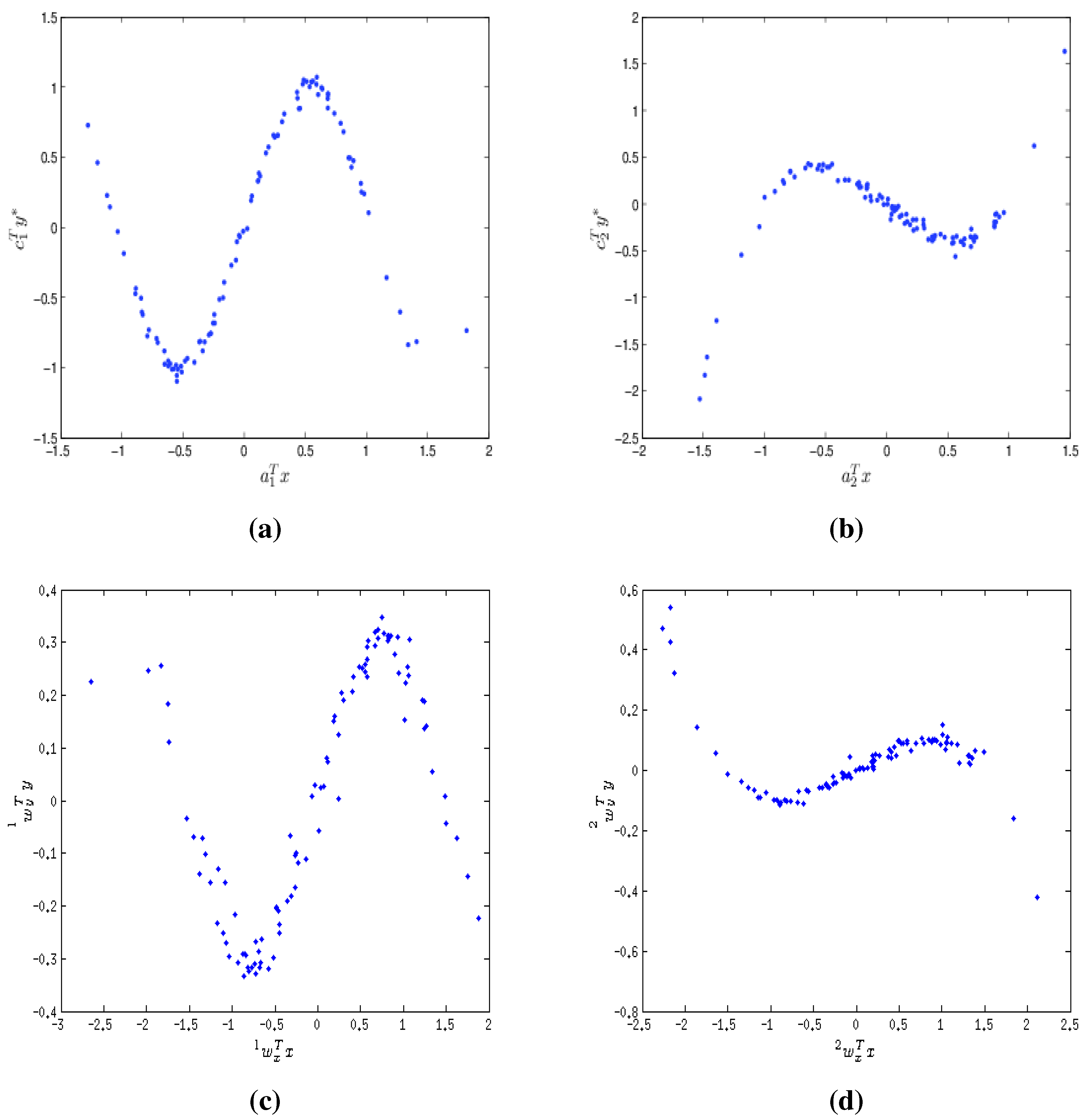
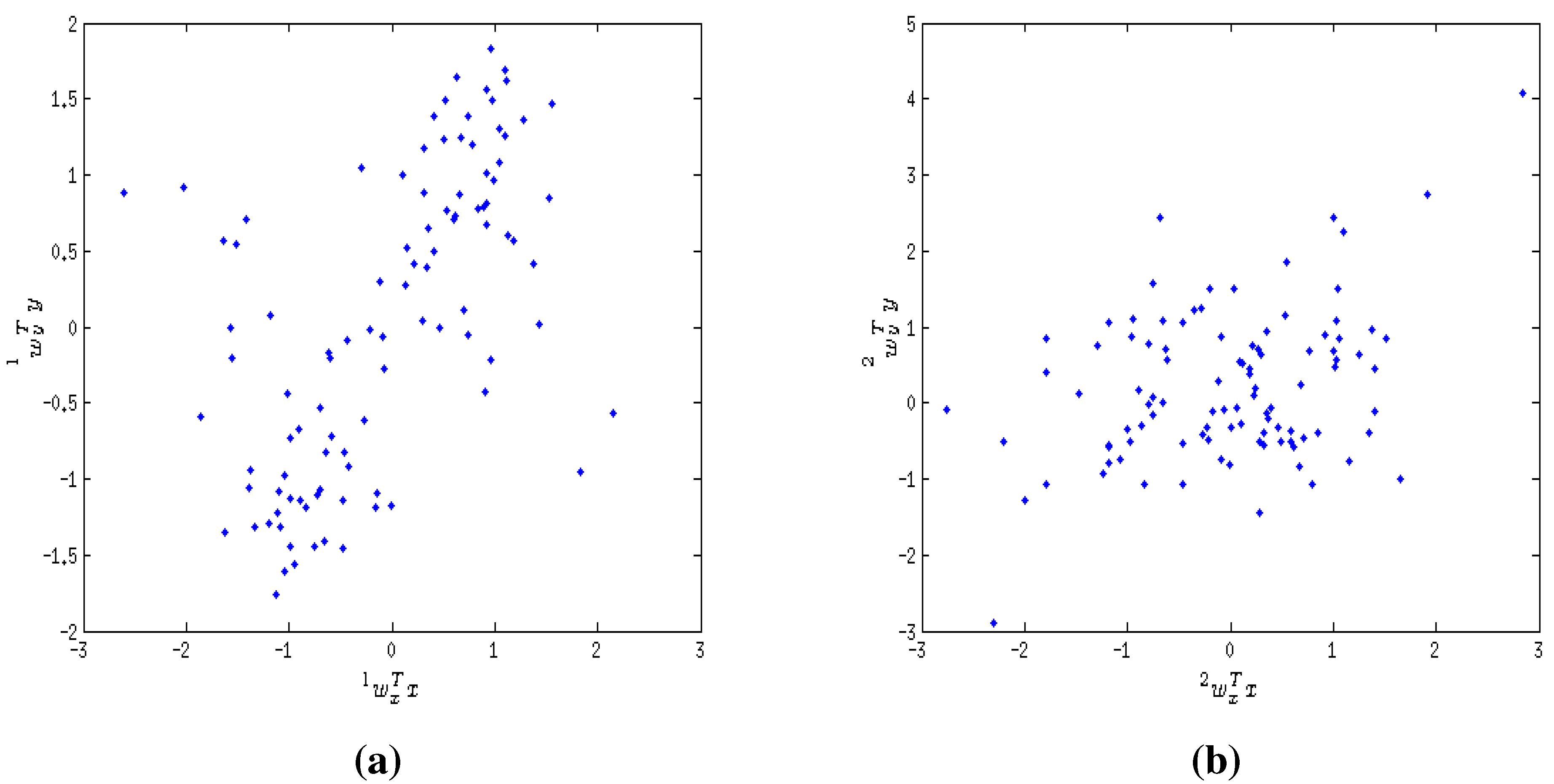
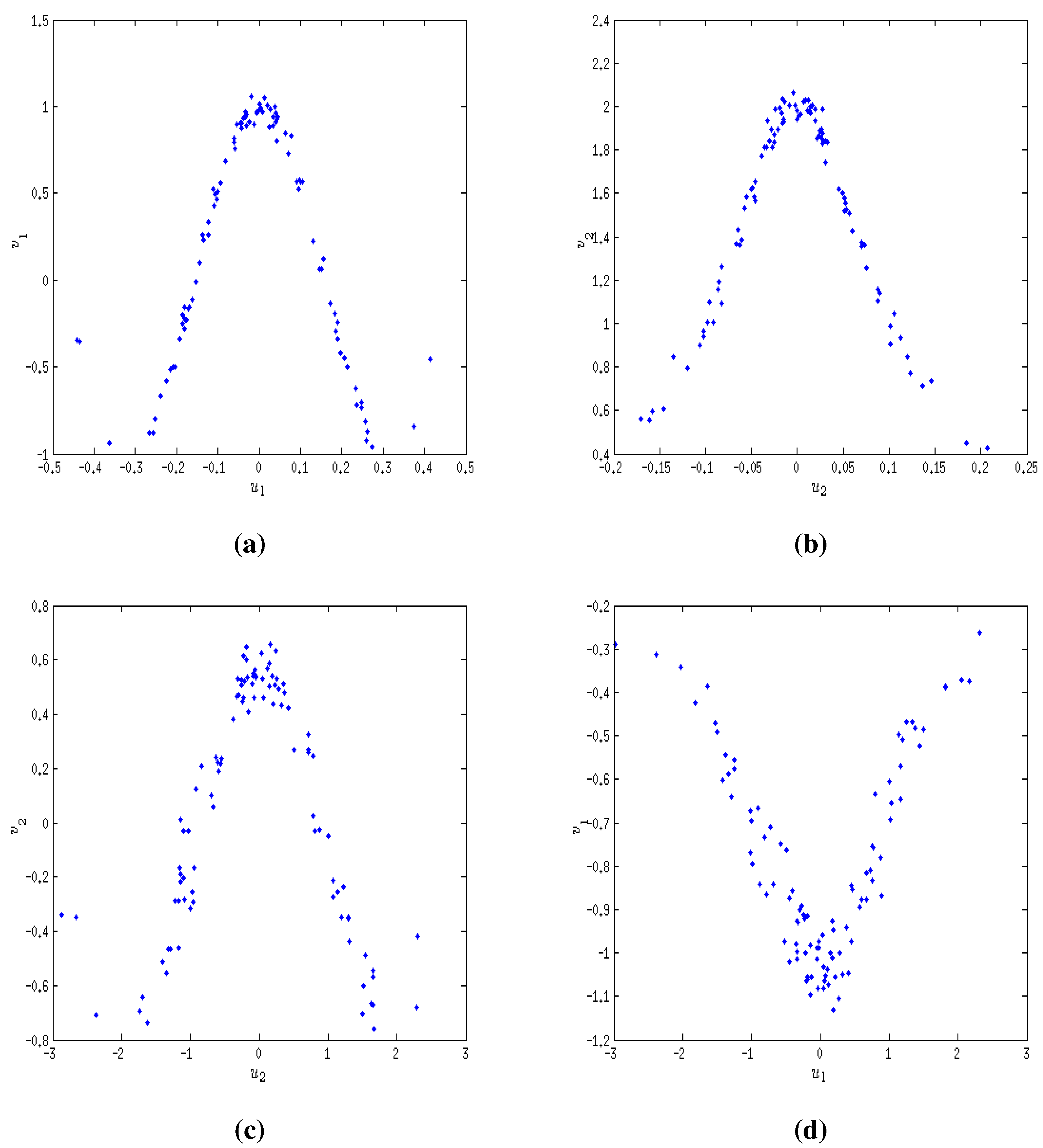
9.1. Extraction of Non-linear Relationship

Example 1: The dimensions of $\mathbf{x}$ and $\mathbf{y}$ are taken as six and four, respectively; so, $\mathbf{x}={(x_1,x_2,\cdots ,x_6)}^T$ and $\mathbf{y}={(y_1,y_2,y_3,y_4)}^T$. $\mathbf{x}$ is the explanatory variable, where the components are generated from independent $N(0,1)$ random variables. $\mathbf{y}$ is the dependent variable based on the following latent variables:

$$\begin{array}{ccc}\hfill y_1^{*}& =& sin\left(3{\mathbf{a}}_1\mathbf{x}\right)+{ϵ}_1,\hfill \end{array}$$

(44)

$$\begin{array}{ccc}\hfill y_2^{*}& =& {\left({\mathbf{a}}_2\mathbf{x}\right)}^3-{\mathbf{a}}_2\mathbf{x}+{ϵ}_2,\hfill \end{array}$$

(45)

where ${ϵ}_1$ and ${ϵ}_2$ are the random errors, and we assume ${ϵ}_i\sim 0.05N(0,1),i=1,2$. The coefficient vectors, ${\mathbf{a}}_1$ and ${\mathbf{a}}_2$, are generated from independent uniform $(-1/2,1/2)$ random variables, and then, they are orthogonalized. Therefore, ${\mathbf{a}}_1^T{\mathbf{a}}_2=0$. The relationship between $\mathbf{y}$ and the latent variables, ${\mathbf{y}}^{*}={(y_1^{*},y_2^{*})}^T$, is assumed to be the linear combination, as mentioned below:

$$y_1={\mathbf{c}}_1^T{\mathbf{y}}^{*},y_2={\mathbf{c}}_2^T{\mathbf{y}}^{*},$$

(46)

and $y_3$ and $y_4$ are independent $N(0,1)$ random variables. The elements of the matrix, $\mathbf{C}=({\mathbf{c}}_1,{\mathbf{c}}_2)$, are generated from independent uniform $(-1/2,1/2)$ random variables, and then, their rows are orthogonalized, so that the columns of ${\mathbf{C}}^{-1}$ become orthogonal. We generate a sample size of 100 from $\mathbf{x}$ and $\mathbf{y}$.

The scatter plots of the latent variables are given in (a) and (b) of Figure 1. We perform ABCA for this data set with divergent parameters, $\alpha =0.5$ and $\beta =0.5$. The first two AB-canonical variable pairs are plotted in (c) and (d) of Figure 1. The values of the first two AB-canonical coefficients are 0.9616 and 0.9301. It is obvious that ABCA extracts the latent variable quite accurately. We notice that the scale and the sign of the canonical vectors cannot be recovered from ABCA. The standard CCA fails to extract them, due to a non-linear relationship with the latent variables. The first two standard canonical variable pairs are plotted in (a) and (b) of Figure 2. The values of the first two canonical coefficients are 0.5704 and 0.3559.

Figure 2. Scatter plots for the first two standard canonical variable pairs. Here, canonical correlation analysis (CCA) fails to reconstruct the non-linear relationship.

Figure 2. Scatter plots for the first two standard canonical variable pairs. Here, canonical correlation analysis (CCA) fails to reconstruct the non-linear relationship.

Figure 3. (a) Simulated data with outliers inside the red circle. (b) Scatter plot for the AB-canonical variable pair.

Figure 3. (a) Simulated data with outliers inside the red circle. (b) Scatter plot for the AB-canonical variable pair.

Figure 4. (a) Scatter plot for the standard canonical variable pair. (b) Scatter plot for the canonical variable pair using Yin (2004) [1] approach.

Figure 4. (a) Scatter plot for the standard canonical variable pair. (b) Scatter plot for the canonical variable pair using Yin (2004) [1] approach.

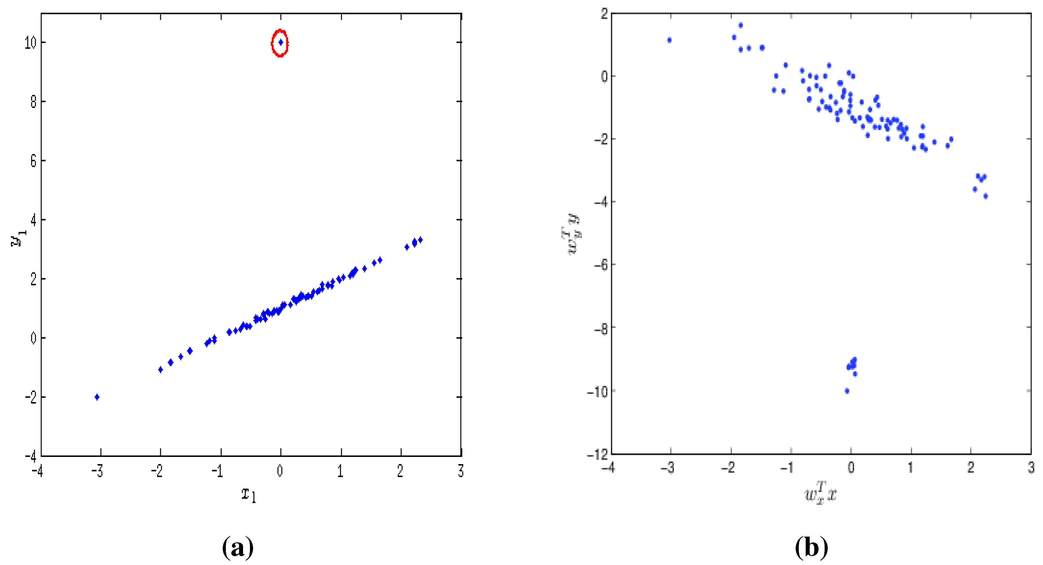
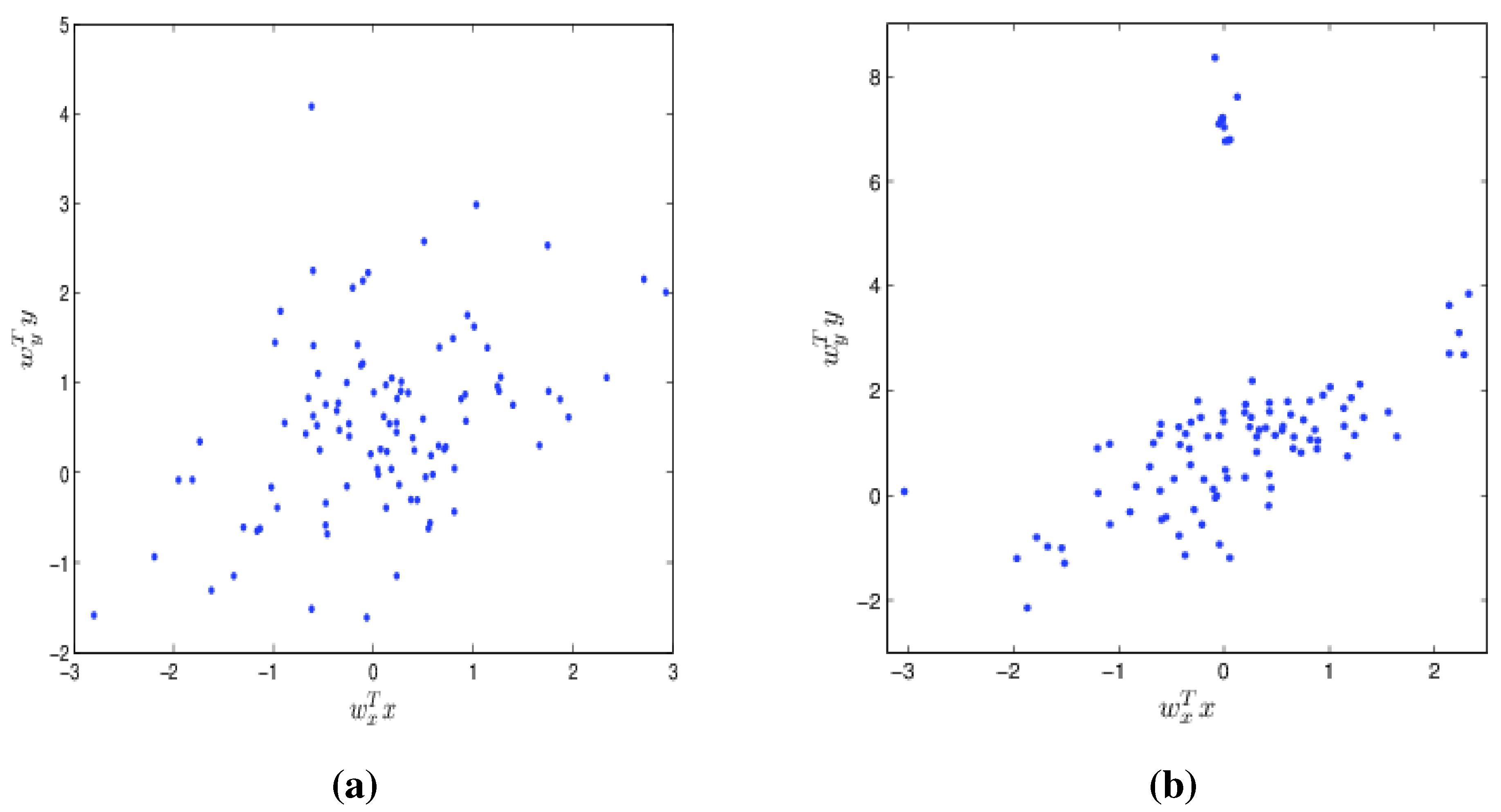
9.2. Robustness Property

Example 2: In this example, we check the robustness property of ABCA. To compare it with standard CCA, we have generated data, such that $\mathbf{x}$ and $\mathbf{y}$ have a linear relationship, and then, few outliers are inserted. The dimensions of $\mathbf{x}$ and $\mathbf{y}$ are taken as five and three, respectively. All the components of $\mathbf{x}$ are generated from independent $N(0,1)$ random variables. For simplicity, we have taken the relationship between $\mathbf{x}$ and $\mathbf{y}$ as follows:

$$y_1=1+x_1+ϵ,$$

(47)

where ϵ is the random error, and we assume $ϵ\sim 0.05N(0,1)$. Here, $y_1$ and $x_1$ are the first components of $\mathbf{x}$ and $\mathbf{y}$, respectively. The other components of $\mathbf{y}$ are generated from independent $N(0,1)$ random variables. We have generated only 90 random samples from this model, and we have taken 10 outliers. For the outlying observations, we have taken $x_1=0$ and $y_1=10$. Figure 3a represents the original data, where there are 10 outlying observations inside the red circle. In Figure 3b, we have plotted the first AB-canonical variable pair. The divergence parameters are taken as $\alpha =0.5$ and $\beta =0.5$. It is seen that ABCA successfully extracts the canonical variables, but Figure 4a shows that the standard CCA completely fails. In Figure 4b, we present the scatter plot of the first pair of the canonical variables using the approach of Yin (2004) [1]. This is based on Kulback-Leibler divergence, so it is a special case of ABCA, where $\alpha =1$ and $\beta =0$. The values of the first AB-canonical coefficients for $\alpha =0.5,\beta =0.5$ and $\alpha =1,\beta =0$ are 0.9121 and 0.7107, respectively. Thus, we can make ABCA robust by choosing suitable tuning parameters.

9.3. Tensor Data

Example 3: In this example, we have generated data from tensor valued random variables, $\underline{\mathbf{X}}$ and $\underline{\mathbf{Y}}$. The dimensions of $\underline{\mathbf{X}}$ and $\underline{\mathbf{Y}}$ are taken as (4,3,2) and (3,2,2), respectively. $\underline{\mathbf{X}}$ is the explanatory variable, where the components are generated from independent $N(0,1)$ random variables. Let us define:

$$u_1=\underline{\mathbf{X}}{\overline{\times }}_1{\mathbf{a}}_x^{\left(1\right)}{\overline{\times }}_2{\mathbf{a}}_x^{\left(2\right)}{\overline{\times }}_3{\mathbf{a}}_x^{\left(3\right)},$$

$$u_2=\underline{\mathbf{X}}{\overline{\times }}_1{\mathbf{b}}_x^{\left(1\right)}{\overline{\times }}_2{\mathbf{b}}_x^{\left(2\right)}{\overline{\times }}_3{\mathbf{b}}_x^{\left(3\right)}.$$

(48)

The vectors, ${\mathbf{a}}_x^{\left(i\right)}$ and ${\mathbf{b}}_x^{\left(i\right)}$, $i=1,2,3$, are generated from independent uniform $(-1/2,1/2)$ random variables, and then, they are orthogonalized. Therefore, ${\mathbf{a}}_x^{\left(i\right)T}{\mathbf{b}}_x^{\left(i\right)}=0,i=1,2,3$. $\underline{\mathbf{Y}}$ is the dependent variable based on the following latent variables:

$$\begin{array}{ccc}\hfill y_1^{*}& =& cos\left(10u_1\right)+{ϵ}_1,\hfill \end{array}$$

(49)

$$\begin{array}{ccc}\hfill y_2^{*}& =& \frac{2}{100u_2^2+1}+{ϵ}_2,\hfill \end{array}$$

(50)

where ${ϵ}_1$ and ${ϵ}_2$ are the random errors, and we assume ${ϵ}_i\sim 0.05N(0,1),i=1,2$. The relationship between $\underline{\mathbf{Y}}$ and the latent variables, ${\mathbf{y}}^{*}={(y_1^{*},y_2^{*})}^T$, is assumed to be the linear combination, as follows:

$$y_{1,1,1}={\mathbf{c}}_1^T{\mathbf{y}}^{*},y_{2,2,2}={\mathbf{c}}_2^T{\mathbf{y}}^{*},$$

(51)

All other components of $\underline{\mathbf{Y}}$ are independent $N(0,1)$ random variables. The elements of the matrix, $\mathbf{C}=({\mathbf{c}}_1,{\mathbf{c}}_2)$, are generated following the way we did in Example 1. We have generated a sample size of 100 from $\underline{\mathbf{X}}$ and $\underline{\mathbf{Y}}$.

The scatter plots of the latent variables are given in Figure 5a,b. We have performed tensor ABCA for this data set with divergent parameters, $\alpha =0.5$ and $\beta =0.5$. The first two tensor AB-canonical variable pairs are plotted in Figure 5c,d. The values of the first two tensor AB-canonical coefficients are 0.98671 and 0.9712. It is obvious that ABCA extracts the latent variable quite accurately.

Figure 5. (a) and (b): The scatter plots of the latent variables. (c) and (d): The scatter plots of the first two tensor AB-canonical variable pairs. It is clearly seen that the non-linear relationship is reconstructed.

Figure 5. (a) and (b): The scatter plots of the latent variables. (c) and (d): The scatter plots of the first two tensor AB-canonical variable pairs. It is clearly seen that the non-linear relationship is reconstructed.

9.4. Choice of Divergence Parameters

There does not exist any universal way of selecting divergence parameters, α and β. They generally control the trade-off between the efficiency and robustness properties of the procedure. Although they cover the whole two-dimensional plane, the rate of change in the values of AB-divergence coefficients for very high or very small values of the tuning parameters are very slow. Therefore, we are often interested in choosing the parameters in the interval [0, 1]. For $\alpha =1$ and $\beta =1$, the AB-divergence turns out to be the $L_2$-distance between two densities. $L_2$-distance is regarded as a strong robust divergence in the literature, but the robustness is achieved at some loss of efficiency (Basu et al., 1998 [13]; Scott, 2001 [31]). On the other hand, for $\alpha =0$ and $\beta =0$, the AB-divergence becomes the $L_2$-distance between the logarithm of two densities, which may be regarded as non-robust. Therefore, a suitable choice of the parameters are needed to balance between robustness and efficiency. In our simulation examples, α and β around $(0.5,0.5)$ seem to a good choice.

10. Conclusion

We have used AB-divergence measure to perform the canonical correlation analysis. It can extract the hidden non-linear relationship between two sets of data, whereas the standard CCA is designed to find out only the linear relationship. Moreover, the standard CCA is very non-robust against the outlying observations. On the other hand, by choosing suitable tuning parameters, α and β, for the AB-divergence, we can make ABCA robust against outliers. Our method is very general in the sense that it uses AB-divergence, which is a general measure of discrepancy. Moreover, we have generalized the method in the case of tensor data, and we have also considered the sparseness constants.

References

1. Yin, X. Canonical correlation analysis based on information theory. J. Multivar. Anal. 2004, 91, 161–176. [Google Scholar] [CrossRef]
2. Yin, X.; Sriram, T. Common canonical variates for independent groups using information theory. Stat. Sin. 2008, 18, 335–353. [Google Scholar]
3. Iaci, R.; Sriram, T.; Yin, X. Multivariate association and dimension reduction: A generalization of canonical correlation analysis. Biometrics 2010, 66, 1107–1118. [Google Scholar] [CrossRef] [PubMed]
4. Iaci, R.; Sriram, T. Robust multivariate association and dimension reduction using density divergences. J. Multivar. Anal. 2013, 117, 281–295. [Google Scholar] [CrossRef]
5. Wang, X.; Crowe, M.; Fyfe, C. Dual stream data exploration. Int. J. Data Min., Model. Manage. 2012, 4, 188–202. [Google Scholar] [CrossRef]
6. Cichocki, A.; Cruces, S.; Amari, S.I. Generalized alpha-beta divergences and their application to robust nonnegative matrix factorization. Entropy 2011, 13, 134–170. [Google Scholar] [CrossRef]
7. Lai, P.L.; Fyfe, C. Kernel and nonlinear canonical correlation analysis. Int. J. Neural Syst. 2000, 10, 365–377. [Google Scholar] [CrossRef] [PubMed]
8. Shawe-Taylor, J.; Cristianini, N. Kernel Methods for Pattern Analysis; Cambridge University Press: Cambridge, UK, 2004. [Google Scholar]
9. Breiman, L.; Friedman, J.H. Estimating optimal transformations for multiple regression and correlation. J. Am. Stat. Assoc. 1985, 80, 580–598. [Google Scholar] [CrossRef]
10. Hotelling, H. Relations between two sets of variates. Biometrika 1936, 28, 321–377. [Google Scholar] [CrossRef]
11. Amari, S.I. Integration of stochastic models by minimizing α-divergence. Neural Comput. 2007, 19, 2780–2796. [Google Scholar] [CrossRef] [PubMed]
12. Mihoko, M.; Eguchi, S. Robust blind source separation by beta divergence. Neural comput. 2002, 14, 1859–1886. [Google Scholar] [CrossRef] [PubMed]
13. Basu, A.; Harris, I.R.; Hjort, N.L.; Jones, M. Robust and efficient estimation by minimising a density power divergence. Biometrika 1998, 85, 549–559. [Google Scholar] [CrossRef]
14. Cichocki, A.; Zdunek, R.; Amari, S.I. Csiszár’s divergences for non-negative matrix factorization: Family of new algorithms. In Independent Component Analysis and Blind Signal Separation, Proceedings of Fifth International Conference, ICA 2004, Granada, Spain, 22–24 September 2004; Puntonet, C.G., Prieto, A., Eds.; Springer: Berlin, Heidelberg, Germany, 2006; pp. 32–39. [Google Scholar]
15. Kompass, R. A generalized divergence measure for nonnegative matrix factorization. Neural comput. 2007, 19, 780–791. [Google Scholar] [CrossRef] [PubMed]
16. Févotte, C.; Bertin, N.; Durrieu, J.L. Nonnegative matrix factorization with the Itakura-Saito divergence with application to music analysis. Neural Comput. 2009, 21, 793–830. [Google Scholar] [CrossRef] [PubMed]
17. Scott, D.W. Multivariate Density Estimation: Theory, Practice, and Visualization; Wiley: New York, NY, USA, 1992; Volume 1. [Google Scholar]
18. Silverman, B.W. Density Estimation for Statistics and Data Analysis; Chapman & Hall/CRC: London, UK, 1986; Volume 26. [Google Scholar]
19. Kim, J.S.; Scott, C. Robust kernel density estimation. J. Mach. Learn. Res. 2012, 13, 2529–2565. [Google Scholar]
20. Byrd, R.H.; Hribar, M.E.; Nocedal, J. An interior point algorithm for large-scale nonlinear programming. SIAM J. Optim. 1999, 9, 877–900. [Google Scholar] [CrossRef]
21. Byrd, R.H.; Gilbert, J.C.; Nocedal, J. A trust region method based on interior point techniques for nonlinear programming. Math. Program. 2000, 89, 149–185. [Google Scholar] [CrossRef]
22. MATLAB code of ABCA. Available online: http://www.isical.ac.in/∼abhijit_v/ABC.m (accessed on 17 July 2013).
23. Efron, B.; Tibshirani, R.J. An Introduction to the Bootstrap; Chapman & Hall/CRC: New York, NY, USA, 1993; Volume 57. [Google Scholar]
24. Davison, A.C.; Hinkley, D.V. Bootstrap Methods and Their Application; Cambridge University Press: Cambridge, UK, 1997; Volume 1. [Google Scholar]
25. Kolda, T.G.; Bader, B.W. Tensor decompositions and applications. SIAM rev. 2009, 51, 455–500. [Google Scholar] [CrossRef]
26. Cichocki, A.; Zdunek, R.; Phan, A.H.; Amari, S.I. Nonnegative Matrix and Tensor Factorizations: Applications to Exploratory Multi-way Data Analysis and Blind Source Separation; Wiley: Chichester, UK, 2009. [Google Scholar]
27. Torres, D.A.; Turnbull, D.; Barrington, L.; Lanckriet, G.R. Identifying words that are musically meaningful. In Proceedings of the 8th International Conference of Music Information Retrieval, Vienna, Austria, 23–27 September 2007; Volume 7, pp. 405–410.
28. Witten, D.M.; Tibshirani, R.; Hastie, T. A penalized matrix decomposition, with applications to sparse principal components and canonical correlation analysis. Biostatistics 2009, 10, 515–534. [Google Scholar] [CrossRef] [PubMed]
29. Witten, D.M. A penalized matrix decomposition, and its applications. PhD thesis, Stanford University, USA, 2010. [Google Scholar]
30. Allen, G.I. Sparse higher-order principal components analysis. In Proceedings of 15th International Conference on Artificial Intelligence and Statistics, Canary Islands, Spain, 20–22 April 2012; Volume 22, pp. 27–36.
31. Scott, D.W. Parametric statistical modeling by minimum integrated square error. Technometrics 2001, 43, 274–285. [Google Scholar] [CrossRef]