Element Composition of Fractionated Water-Extractable Soil Colloidal Particles Separated by Track-Etched Membranes

Abstract

Membrane fractionation with track-etched membranes was used to size-profile the microelement composition of water-extractable soil colloids (WESCs). The aim of the study is the element composition of narrow WESC fractions of typical chernozems in the range of 0.01–10 µm. Micro-/ultrafiltration through a cascade of track-etched polycarbonate membrane filters with pore sizes of 5, 2, 1, 0.8, 0.4, 0.2, 0.1, 0.05, 0.03, and 0.01 µm at room temperature was used. ICP–AES using direct spraying of obtained fractions without decomposition was used; Al, Ba, Cd, Cr, Cu, Fe, Mn, Si, Sr, Ti, Zn, Ca, K, Mg, Na, P, and S were found. Narrow WESC fractions differ significantly. For macro- and microelements, maximum amounts of Si, Al, Fe, and Ti and their maximum percentages are observed in fractions with sizes above 1 µm, while Ca, Mg, Mn, Cu, Zn, K, and S are accumulated more in fractions with sizes below 1 µm. The developed approach provides preparative isolation of a detailed set of narrow WESC fractions in the micrometer–nanometer range. This provides element soil profiles that reveal distinct differences and the individual character of each fraction as well as trends in changes in the mineral matrix and microelement composition with fraction size.

1. Introduction

The circulation of soil particles on surfaces, in ground waters, and in soils depends on their size [1,2]. The study of the composition and properties of soil colloids has almost a century of history, which is associated with their active participation in soil-forming processes and the formation of a soil absorbing complex [3,4]. Colloids are considered particles with sizes of ca. 1 nm to 1–2 µm [5,6], i.e., the silty fraction of soils, sometimes including fine dust particles up to 10 µm [7,8]. They consist of substances of inorganic, organic, and organo-clay nature [9,10] and are frequently considered particulate soil organic matter (SOM) [11]. These colloids show large specific surface areas and high sorption capacities and migration activities, which lead to their transfer from the soil profile to adjacent environments, groundwater, and other natural waters. Adsorbed inorganic (heavy metals, phosphates) [12,13] and organic (pesticides, PAHs, etc.) contaminants [14] may thus be transported over long distances, spreading pollutants in soil and aqueous media and increasing or minimizing environmental risks, depending on the material composition and colloids and their affinity for pollutants [7,15].

A broad range of particle sizes of the colloidal fraction (1 nm–1 or 10 µm) includes subfractions of particles of different mineralogical and chemical compositions, which also differ in their sorption capacity and migration activity [16,17,18]. All this necessitates a detailed study of the composition of such subfractions of migratory-active particles that readily turn into aqueous extracts. Due to the complex composition of the colloidal fraction, it becomes necessary to develop the methodology, including methods for sample preparation and data processing. There are two main approaches to studying these natural disperse systems [19], which show both the heterogeneity of the chemical composition at the molecular level and the complexity of the structure at the macroscopic scale: the system can be considered either as a chemical continuum or a mixture of various components that can be separated (fractionated) and studied separately.

Thus, techniques such as sieve analysis, microfiltration, and variations of microscopic methods are used to analyze particulate SOM [11,20]. These methods allow one to study particles up to 500 µm. For dissolved SOM, methods such as dialysis [21,22], ultra- and nanofiltration, reverse osmosis [23], and high-performance gel-permeation and size exclusion chromatography [24,25] can be used. The mineral part is often analyzed using methods such as atomic emission or IR spectroscopies [26].

Among these methods, membrane filtration is technically simplest; however, it is an effective approach. Filtration through membranes with a pore size of 0.22 or 0.45 µm has long been used to isolate particulate SOM, so-called water-extractable soil colloids (WESCs). However, there are almost no studies using a broad range of membranes with different pore sizes for separating and concentrating WESC fractions.

Track-etched membranes are of particular interest for solving this problem. The use of this membrane type goes back to the 1970s [27,28]. The use and fabrication of track-etched membranes for fine fractionation became widespread in the 1990s [29,30]. Among the advantages of this technique are higher extraction values of dissolved organic matter compared with other fractionation methods [31], no complex sample preparation, ease of use in many respects, and a broad range of membranes with different pore sizes. At the same time, it is noted [32] that one of the main disadvantages of membrane filtration is significant differences in the extraction of organic matter when using different ultrafiltration systems and experimental conditions. However, this type of membrane is rarely applied to SOM; in a recent review [33], only 1 out of 30 papers [34] used polycarbonate track-etched membranes to remove organic matter in the process of water purification due to a hybrid process of electrocoagulation and dead-end microfiltration.

This work is aimed at assessing the possibility of separating the water-extractable part of soil colloids using a broad-range set of membrane filters with pore sizes of 0.01 to 10 µm, concentrating narrow fractions, the efficiency and reproducibility of such separation based on atomic emission spectrometry using polycarbonate membrane filters, as well as assessing the composition and role of the selected fractions in the total pool of water-extractable soil colloids.

2. Materials and Methods

2.1. Chemicals and Samples

All aqueous solutions were prepared using Type I deionized water (18.2 MΩ cm at 25 °C) obtained using a Milli-Q Academic system (Merck Millipore, Darmstadt, Germany). Sodium azide (purity > 99.5%, Molekula Ltd., Darlington, UK) was used as a preservative agent for obtained samples. Samples were acidified with 69% nitric acid (PA-ACS-ISO grade, Panreac, Barcelona, Spain). For obtaining water-extractable soil organic matter, samples of Kursk chernozem (V.V. Alekhin Tsentralno-Chernozemny Nature Reserve of Russia) were used [35,36].

2.2. Fractionation Setup

For sequential membrane filtration, a set of polycarbonate track-etched membranes (GVS Filter Technology, Bologna, Italy) was used, nominal pore size, 5.0, 2.0, 1.0, 0.8, 0.4, 0.2, 0.1, 0.05, 0.03, and 0.01 µm. Membrane fractionation was carried out using a system consisting of two 1 L vacuum filtration flasks (Figure 1), one of which was equipped with a stainless-steel frit and funnel (Rocker Scientific Co., Ltd., Kaohsiung, Taiwan); the other had a porous glass filter, glass funnel, and an aluminum clamp (Borosil Ltd., Mumbai, India). Filtration was performed using a Rocker 410 oil-free vacuum pump (Rocker Scientific Co., Ltd., Kaohsiung, Taiwan).

An AS 200 sieving machine (Retsch, Haan, Germany) with sieves of 40, 20, 10, and 5 µm (Precision Eforming LLC., Cortland, NY, USA) was used for preliminary sieving of soil samples (Figure S1, Supplementary Information). After the initial sieving at an amplitude of 0.85 mm (time, 5 min), the set of sieves was washed with 50 mL of deionized water and the sample was sieved for another 5 min at the same amplitude.

2.3. ICP–AES Measurements

For element analysis of the size fractions, an axial ICP–OES 720-ES instrument (Agilent Technologies, Santa Clara, CA, USA) was used. The spectrometer was equipped with an SPS3 autosampler (Agilent Technologies, Santa Clara, CA, USA), a low-flow axial quartz torch with a 2.4 mm inner diameter injector tube, a double-pass glass cyclonic spray chamber, a polypropylene pneumatic nebulizer (OneNeb, Agilent Technologies, Santa Clara, CA, USA), and a Trident Internal Standard Kit (Glass Expansion, Pocasset, MA, USA). A peristaltic pump used a white/white PVC pump tube for feeding and a blue/blue one for the drain. The measurement parameters are summed up in

Table 1. Conditions of ICP–AES measurements.

Parameter	Value
Measurement conditions
Power, kW	1.30
Plasma flow, L/min	18.0
Axial flow, L/min	1.50
Nebulizer flow, L/min	0.95
Replica reading time, s	25
Stabilization time, s	35
Replicates	3
Sample introduction parameters
Sample introduction delay, s	20
Wash time, s	5
Pump, rpm	12

. Emission lines from Table S1 (Supplementary Information) were used for measurements. All lines were measured simultaneously (a MultiCal mode). Results were collected and processed using ICP Expert software 2.0.5 (Agilent Technologies, Santa Clara, CA, USA). Linear or quadratic functions were used for calibration.

A multielement standard solution of 24 elements; ICP-AM-6 (Ag, Al, Sb, Ba, Be, B, Cd, Ca, Cr, Co, Cu, Fe, Pb,100, Li, Mg, Mn, Ni, K, Si, Na, Sr, Tl, V, and Zn) with a concentration of each element of 100 mg/L (High-Purity Standards, North Charleston, SC, USA); a multielement standard solution of 4 elements; ICP-AM-15 (Na, K, Ca, Mg) with a concentration of each element of 10,000 mg/L (High-Purity Standards); single element standard solutions of P, S, and Si with concentrations of 1000 mg/L (Inorganic Ventures, Christiansburg, VA, USA); and single element standard solution of Fe with concentrations of 10,000 mg/L (High-Purity Standards) were used for calibration. Concentration ranges of elements in the calibration solutions were 0.04–20 mg/L for Ag, Al, As, B, Ba, Be, Cd, Co, Cr, Cu, Li, Mn, Mo, Ni, Pb, Sb, Se, Sn, Sr, Ti, V, W, and Zn; 0.04–400 mg/L for Ca, Fe, K, Mg, and Na; 0.4–200 mg/L for P and S; and 10–200 mg/L for Si. A scandium standard solution (10,000 mg/L; Inorganic Ventures, Christiansburg, VA, USA) was used as an internal standard (20 mg/L). Nitric acid (69%, PA-ACS-ISO grade, Panreac, Barcelona, Spain) was used as a diluent for calibration standards.

2.4. Procedures

2.4.1. Membrane Leaching

Using a system consisting of a Bunsen flask, a special funnel, and a water jet pump, 250 mL of deionized water for membranes with a pore size of 1 µm and 150 mL for a membrane of 0.01 µm (due to the time of the filtration process) were passed through track polycarbonate membranes. Then, membranes were subjected to a procedure similar to washing off particles during cascade filtration: The membrane was placed in a clean beaker, 10 mL of deionized water was added to it, then the membrane was exposed to ultrasound for 3 min at the lowest possible power of the ultrasonic bath, after which the liquid was transferred into a volumetric flask of 25.00 mL. Two portions of deionized water (7–10 mL) were again added to the membrane in succession, and the process of exposure to ultrasound was repeated; then, the volume of the flask was adjusted to the mark with a washing solution or deionized water. The resulting fractions were transferred to 100 mL flasks, stored at +4 °C, and then analyzed.

2.4.2. Extraction of the Colloidal Fraction

For a cold extract, a 40 g sample of chernozem, previously ground in a jasper mortar, was placed in a 700 mL Erlenmeyer flask. Then, 400 mL of deionized water at room temperature (1 g soil per 10 mL of deionized water) was added [1]. The resulting suspension was shaken with a laboratory shaker for 1 h [37] and then left for 30 min.

2.4.3. Size Fractionation

For fractionation of the obtained extract, analytical polycarbonate track-etched membranes were used. Then, sequential membrane filtration was carried out using membranes with pore sizes of 5, 2, 1, 0.8, 0.4, 0.2, 0.1, 0.05, 0.03, and 0.01 µm for polycarbonate analytical track membranes. The general scheme of fractionation is shown in Figure S1 (Supplementary Information). The extract was subjected to cascade filtration, starting from membranes with larger pore sizes (5.0 µm→…→0.01 µm). Before each filtration step, the system was flushed extensively with 100 mL of deionized water to flush out the plasticizer from membranes and clean the vessels. The filtrates were collected in clean containers of 500 mL (not adjusted to the mark) and filtered further. Fractions > 10, 5–10, 2–5, 1–2, 0.8–1, 0.4–0.8, 0.2–0.4, 0.1–0.2, 0.05–0.1, 0.03–0.05, 0.01–0.03, and <0.01 µm were obtained.

2.4.4. Washing from Membranes

To wash off particles concentrated on the membrane due to filtration, it was placed in a clean beaker and 8 mL of deionized water was added. Then, particles were washed off using an ultrasonic bath for 3 min at minimum power. Next, the suspension was transferred into a volumetric flask of 50.00 mL for a fraction of 2–5 µm or 25.00 mL for the rest. Two portions of deionized water (7–10 mL) were again added to the membrane in succession, and the process of washing off the particles was repeated; then, the volume was adjusted to the mark with a washing solution or deionized water. The following fractions were obtained: 2–5, 1–2, 0.8–1, 0.4–0.8, 0.2–0.4, 0.1–0.2, 0.05–0.1, 0.03–0.05, 0.01–0.03, and <0.01 µm. The fractions were transferred into 100 mL vessels and stored at +4 °C.

2.5. Data Treatment

To compare the element contents in the obtained fractions, the concentrations were recalculated for the mass of the sample of soil. The recalculation of metal concentrations per soil sample is described in the Supplementary Information.

Simple correlation analysis was made using Origin Pro software (OriginLab, Northampton, MA, USA). Cluster and factor analyses of the distribution of the molar content of elements were made using Statistica 13.5 software (Tibco, Palo Alto, CA, USA). The distribution of the fractional content of elements in the fractions was analyzed: x_m = a_m/Σ(a₁…a_n), where x_m is the fraction of the element in the size fraction, a_m is the element content in the fraction, and Σ(a₁…a_n) is the total content of the element.

3. Results

In the first stage, the effects of the membrane material on the resulting fractions were studied, since, in addition to the main component (in this case, polycarbonate), a plasticizer and admixtures are present in the membranes. With ICP–AES, the content of elements was determined in wash water. All the elements that were then determined in fractions, Ag, Al, As, B, Ba, Be, Cd, Co, Cr, Cu, Fe, Li, Mn, Mo, Ni, Pb, Sb, Se, Si, Sn, Sr, Ti, Tl, V, W, Zn, Zr, Ca, K, Mg, Na, P, and S, were not detected at the level of 10 µg/L, which is the lower quantification limit for most of these elements by ICP–AES. Thus, the impact of membrane material can be considered insignificant for the results of this study. However, a procedure for washing with 100 mL of deionized water was used (Section 2.4.1) to warrant the absence of any contribution from membranes.

In the obtained narrow fractions, Al, Ba, Cd, Cr, Cu, Fe, Mn, Si, Sr, Ti, Zn, Ca, K, Mg, Na, P, and S were found. The content of other elements was below the detection limits. The sodium content in the fractions was primarily due to the addition of sodium azide as a preservative; therefore, Na was not measured. Thus, the following elements were considered: Al, Ba, Cd, Cr, Cu, Fe, Mn, Si, Sr, Ti, Zn, Ca, K, Mg, P, and S. From the correlation map (Figure 2), the detected elements can be divided into four sets by the correlation coefficients with Si (silicate):

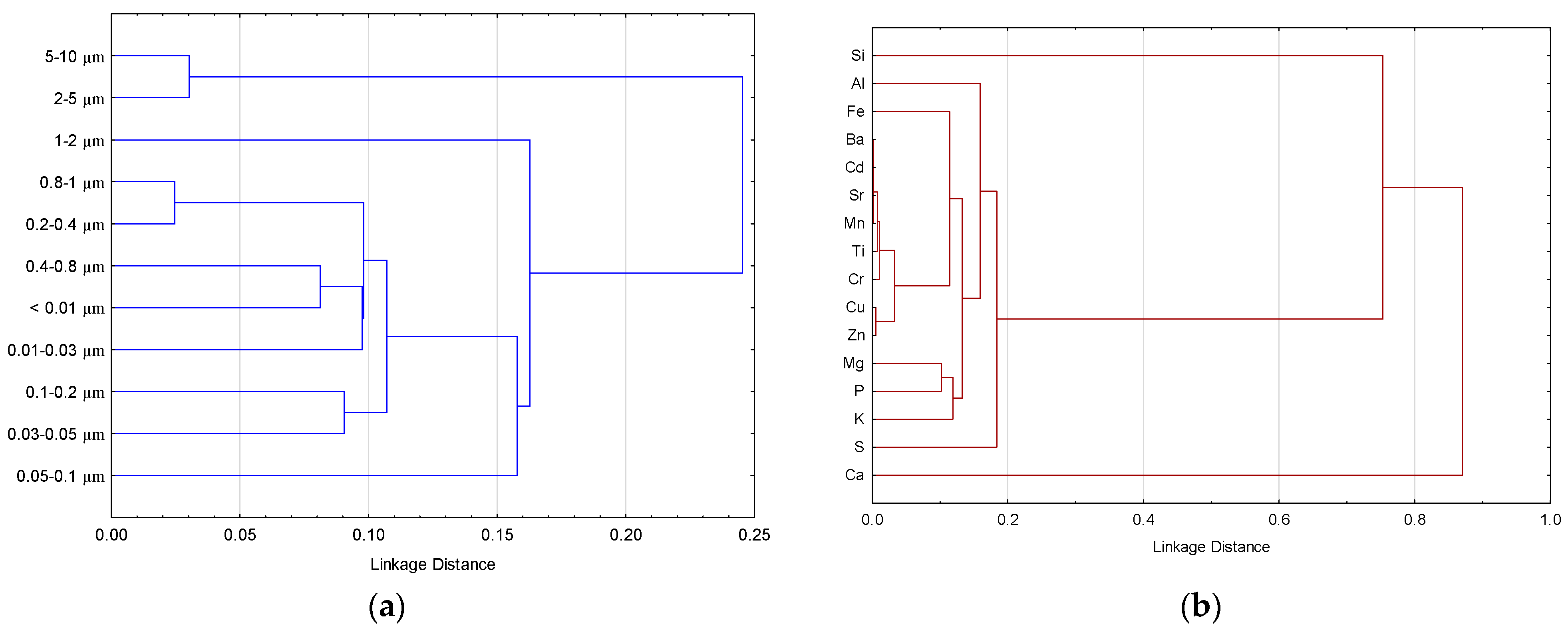
• Si, Al, and Fe as silicate matrix elements and Ti and Mn with correlation coefficients with Si, Al, and Fe above 0.9. The elements of this set are shaded in magenta (Figure 2).
• Ca and S (as other main elements), and Cd and also Cr, with strongly negative correlation coefficients with the matrix elements of Set 1 and shaded blue (Figure 2).
• Mg, Sr, K, and P, and also Ba, showing high correlation coefficients within the group, correlation coefficients with Set 1 over 0.5, and shaded violet (Figure 2).
• Cu and Zn showing a good correlation between one another and very low correlation coefficients with other groups. The set is shaded yellow (Figure 2).

Element profiles as concentration vs. particle size are presented in Figure 3, Figure 4, Figure 5 and Figure 6. The whole distribution of the studied elements is given in Figure 7. Molar ratios for the macroelements are summed up in Figure 8. The results of factor analysis of all the elements are shown in Figure 9. The whole profile of elements (Figure 7) shows that there are seven main elements in total with the concentrations in the majority of fractions above 5% w/w: Si, Al, Fe, Ca, S, Mg, and K. Among them, two elements predominate: calcium and silicon (Figure 7). According to Figure 2, these two elements show a rather strong negative correlation, which is due to the predominantly non-silicate, carbonate nature of calcium in chernozem soil. Because a sample of the upper layer was taken for analysis, carbonates are not crystallized or weakly crystallized, do not stand out morphologically, and exist mainly in the form of impregnation, i.e., they are associated with the readily soluble fine part. Silicon is predominant in particles larger than 1 µm, while calcium is predominant in particles below 1 µm.

The levels of potassium, sulfur, and phosphorus are almost the same for all fractions, while iron and aluminum contents obviously correlate with silicon.

At the same time, the ratios do not fully correspond to the concentrations of these elements, and the amounts of both silicon and calcium differed for different size fractions: they both accumulate in the largest and smallest fractions (Figure 3 and Figure 4), which correlates with the total amounts of elements in the studied range (Figure 10). Thus, all the fractions can be divided into the largest fraction of 5–10 µm; the final filtrate of ca. 15% of the whole mass of elements; and the rest of fractions with approximately equal concentrations of 0.5–2% of the concentration in the largest fraction. It is worth mentioning that the total concentration of elements in the fractions from 1 µm to 0.01 µm does not depend on the particle size (Figure 10).

From the viewpoint of individual element mass distributions (Figure 3, Figure 4, Figure 5 and Figure 6), all the fractions can also be divided into three parts: large fractions of 5–10 and 2–5 µm with the domination of silicate-based elements, small fractions from 1 µm to 0.01 µm with the domination of calcium and sulfur, and the fraction of 1–2 µm, which appears to be an average of the composition of the larger and smaller fractions. It is worth mentioning that this change in element distribution correlates well with the total amount of particles found in fractions. Also, all the elements of Sets 1 and 3 (except Ba) show a correlation (coefficient is no less than 0.8) of the concentration of the element and the total amount of elements in this fraction, while all the elements of Sets 2 and 4 show no correlation with the total amount of elements in this fraction. Also, the fraction of 0.03–0.05 µm is different from both larger and smaller fractions, and shows high fractions of all the main elements, both silicate- and sulfate-based. The range of this fraction fits well with the boundary between particulate and dissolved SOM [38].

4. Discussion

4.1. Interelement Correlations

As a whole, the division of the studied elements into four sets according to coefficient of correlations with Si as the matrix elements of the silicate-based chernozem soil has a rather obvious chemical meaning as Set 1 comprises elements that directly accompany Si in the matrix, while Set 3 has less directly related elements that are either hard Pearson’s acids or phosphate (a hard Pearson’s base). The softest acid, barium, shows less correlation with other elements, which makes barium an in-between element of Sets 3 and 4 (Figure 2). Additionally, chromium, which can also be considered an in-between element of Sets 3 and 4, shows not many correlations with other elements. Set 4 is centered around soft Pearson’s acids, Cu and Zn, that form complexes with humic and fulvic acids [39,40,41,42].

On the contrary, Set 2 comprises calcium, one of the main elements of the profile, and total sulfur. Their negative correlations with silicate-matrix elements show that these are calcium-sulfate-based particles. Cadmium, belonging to this set according to correlation analysis, is most probably due to its affinity to sulfide species of sulfur.

Selected sets of elements agree with the results of the distribution of elements in river water studied using flow fractionation with an inductively coupled plasma mass spectrometric detector [43]. The authors divided the studied elements into four groups: (1) dissolved simple anions, (2) elements mostly associated with WESCs of organic carbon, (3) elements mostly associated with iron-based colloidal particles (various iron, aluminum oxides), and (4) elements bonded by both carbon-based WESC particles and iron-based colloidal particles. At the same time, the first set of elements (Si, Al, Fe, Mg, Mn, Ti, as well as Ba) obtained in this work correlates with the third group in [43], Set 4 (Cu and Zn) with the second, and Set 3 (K and Cr) with the fourth group in [43].

4.2. Set 1: Silicon, Aluminum, Iron, Titanium, and Manganese

The elements of this set are closely related to each other; the correlation coefficients for any pair from this set except Mn are higher than 0.98. The correlation coefficient of the Al–Fe pair is especially distinguished (r_Al–Fe = 0.998), which is expected to some extent since aluminum- and iron-bearing minerals often accompany each other in soils [44] due to the coexistence of minerals based on iron oxides, e.g., with kaolinite [45].

Silicon is an integral part of the mineral composition of chernozem. It is present in minerals such as smectite, illite, kaolinite, and other clay minerals [46]. Silicon is predominant in large fractions only, namely 5–10 µm, 1130 ± 10 µg/g (Figure 7). For smaller particles, silicon concentration decreases and does not exceed 6 µg/g, with the exception of the final fraction of <0.01 µm, where its concentration increases to 34.1 ± 0.5 µg/g (Figure 3).

For aluminum, a profile of changes in a concentration almost identical to silicon is observed, r_Al–Si = 0.989, since aluminum often accompanies silicon in various aluminosilicates [46]. Like silicon, aluminum is present predominantly in large fractions (Figure 7). Thus, for a fraction of 5–10 µm, it is 300 ± 20 µg/g. As in the case of silicon, there is a significant decrease in the content of this metal with fraction size, and for fractions below 1 µm, it does not surpass 1 µg/g. It should be noted that along with aluminosilicates and other aluminum-containing minerals, aluminum can also be present in the form of Al³⁺ and AlOH²⁺ complexes with humic and fulvic acids in smaller fractions [47].

As in the case of aluminum and silicon, iron is associated with larger particles (Figure 3). Thus, the concentration of this metal for a fraction of 5–10 µm is 260 ± 10 µg/g for a fraction of 2–5 and 5.0 ± 0.2 µg/g for 1–2 µm. Then, the iron content drops almost tenfold to 19 ± 1 µg/g. For the remaining fractions, the Fe content does not exceed 1 µg/g (Figure 3).

Titanium is most widely represented in soils by its oxide (rutile, anatase, or brookite) or ilmenite [48]. Very strong correlations of titanium with the matrix elements r_Ti–Si = 0.992, r_Ti–Al = 0.999, and r_Ti–Fe = 0.998 can be explained by the presence of substituted aluminosilicates in the soil. For the most part, it is associated with particles larger than 2 µm (Figure 7). The maximum concentration of 19 ± 1 µg/g is observed for the largest fraction, but for other fractions, it does not exceed 0.05 µg/g (Figure 3).

For manganese, the pattern is similar to that of titanium (r_Mn–Ti = 0.885). Manganese shows a strong correlation with the rest of the matrix elements, r_Mn–Si = 0.923, r_Mn–Al = 0.874, and r_Mn–Fe = 0.889. As with the other elements of Set 1, manganese is associated for the most part with particles of 2–10 µm, with a maximum concentration of 5.5 ± 0.6 µg/g, while for particles less than 1 µm, its content is 0.01–0.1 µg/g, and for the smallest fraction, its concentration increases to 0.73 ± 0.09 µg/g.

4.3. Set 2: Calcium, Sulfur, Chromium, and Cadmium

This set opposes the elements of the first set—Si, Al, Fe, Ti, and Mn—and shows strong negative correlations with them (Figure 2). Apart from negative correlations with Set 1, calcium, cadmium, and sulfur show relatively weak but significant correlations between each other.

For all the fractions below 1 µm calcium is a dominating element (Figure 7) and the concentration of calcium is not below 10 µg/g (Figure 4). The profile for calcium is much flatter compared with the elements of the first set (compare Figure 3 and Figure 4). The largest and smallest fractions show much higher concentrations of calcium of 200 µg/g.

Sulfur shows a rather good correlation with calcium (r_Ca–S = 0.700) and also demonstrates a flat profile (Figure 4) at a level of 0.5–1.0 µg/g. As for calcium, the smallest and largest fractions show much higher concentrations, 21 ± 2 and 40 ± 10 µg/g, respectively.

Cadmium shows maximum negative correlations with the elements of Set 1, but rather weak correlations with S and Ca, which may be due to its very low concentrations, below 70 ng/g in all the samples. Still, as cadmium ions and sulfide are soft Pearson’s entities, their correlation is expected. The highest concentration of cadmium in the largest fractions suggests that it is present as insoluble sulfides or oxides.

Chromium content is also low, and its particle-size profile is different from those of the above three elements (Figure 7). For all the fractions with a particle size of less than 1 µm, the concentrations do not differ significantly and do not exceed 0.2 µg/g. For chromium, there is a relatively strong correlation with almost all other elements of Set 2, but it also shows a good correlation with Mg, Sr, and P of Set 3 and no correlation with other elements, like Cu and Zn of Set 4 (Figure 2).

4.4. Set 3: Magnesium, Strontium, Barium, Potassium, and Phosphorus

The highest concentrations for this set were observed for magnesium, potassium, and phosphorus (Figure 7). High correlation coefficients (over 0.9) are observed for pairs of magnesium, strontium, and phosphorus. For potassium, correlation coefficients with these three elements are lower. For barium, the correlation with other elements of this set is low, but it shows the same level of correlation with elements of Set 1. The elements united in this set are related to Set 1 and show moderate correlation coefficients (over 0.5) with the elements of that set (Figure 2). As for the Set 1, these elements are primarily associated with particles larger than 1 µm (Figure 7). Also, the elements of Set 3 show moderate correlations with calcium and chromium (Figure 2).

Magnesium is a fairly common element in soil. It is often found as carbonate minerals (e.g., dolomite) or as various phyllosilicates (e.g., talc or biotite) [49]. Based on the found correlations, it can be assumed that magnesium predominantly exists as silicates; the correlations are slightly higher than those for the Ca–Mg pair. Contrary to the matrix elements of Set 1, magnesium is mostly equally present in all the fractions (Figure 7). Magnesium concentration in other fractions, except for the smallest one, does not exceed 2 µg/g. For the smallest fraction, Mg content increases to 20 ± 1 µg/g.

Strontium behaves similarly to magnesium, showing the largest correlation coefficient (r_Sr–Mg = 0.960). Its concentrations are an order lower than those for Mg, and at the level of 0.1–0.2 µg/g (Figure 5). As for Mg, the Sr content in the smallest fraction is 20 ± 1 µg/g.

Barium is an in-between element of Sets 1 and 3 (Figure 2); its pattern is more similar to those of matrix elements. As with the elements of Set 1, Ba is associated for the most part with particles of 2–10 µm, with maximum concentrations of 0.5–0.7 µg/g (Figure 5). A rather significant negative correlation with sulfur is observed for barium, which has no reliable explanation and may be due to large differences in concentrations of Ba and total sulfur.

Potassium is the element with one of the highest percentages in the total profile (Figure 7) and its content increases with a decrease in the particle size. The concentration profile of K is more similar to those of calcium and sulfur (Figure 4 and Figure 5). The concentration of potassium is at the level of 1–2 µg/g. Like calcium, the largest and smallest fractions show much higher concentrations of potassium of 100 ± 40 and 38 ± 1 µg/g, respectively.

Phosphorus shows strong correlations with the elements of this set, while it exhibits the lowest correlations with the elements of Set 1 (no correlation with manganese). However, it shows rather good correlations with Ca, S, and Cr. Its concentration profile is also flat, and the concentrations are at the level of 1 µg/g, except for the largest fraction, 50 ± 20 µg/g, which evidences either the absorption of phosphates or their existence as rather large particles. As potassium, phosphorus forms a large fraction in the profile for all particle-size fractions (Figure 7).

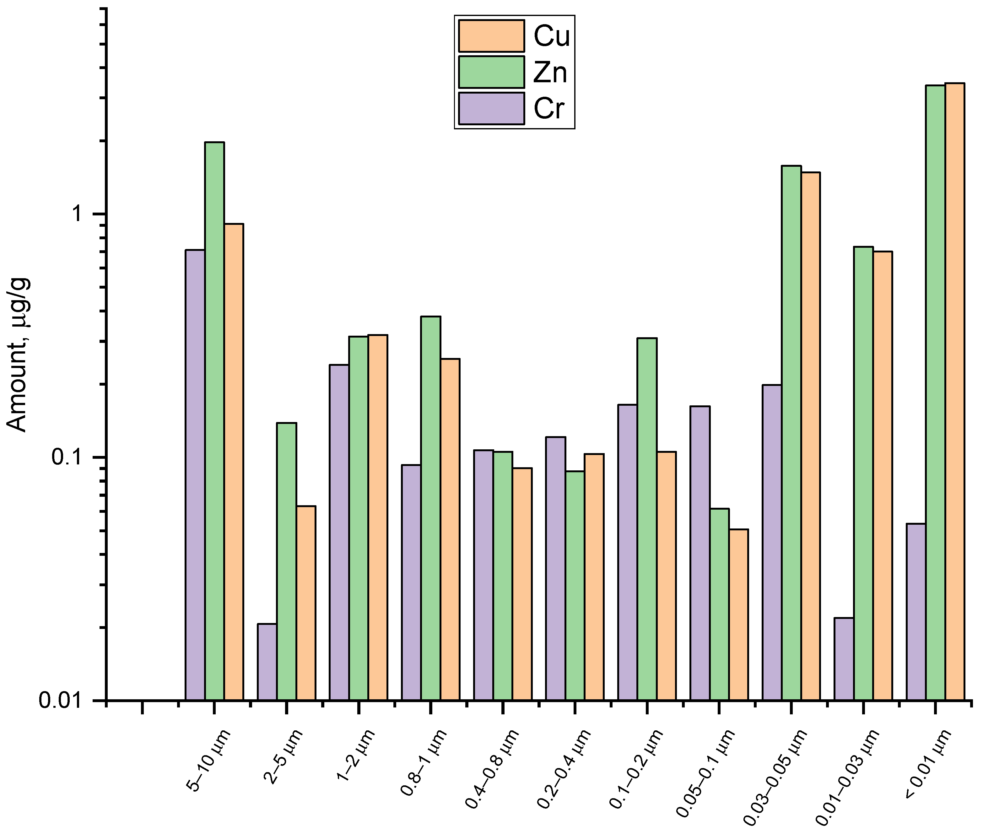
4.5. Set 4: Copper and Zinc

In contrast to the groups above, copper and zinc predominantly correlate with one another only (r_Cu–Zn = 0.998) and show very low correlations with other sets (Figure 2). The main feature is that they are more associated with particles smaller than 0.05 µm (Figure 6). The copper content for the fractions of 0.03–0.05 µm and below are 1.0–3.5 µg/g. For the fraction below 0.01 µm, its concentration is 3.45 ± 0.07 µg/g. The same picture can be seen for zinc; its content is at the same level. For the fraction of below 0.01 µm, its concentration is 3.8 ± 0.1 µg/g. Due to rather large concentrations of copper and zinc, they form a significant part of the three smallest fractions (Figure 7).

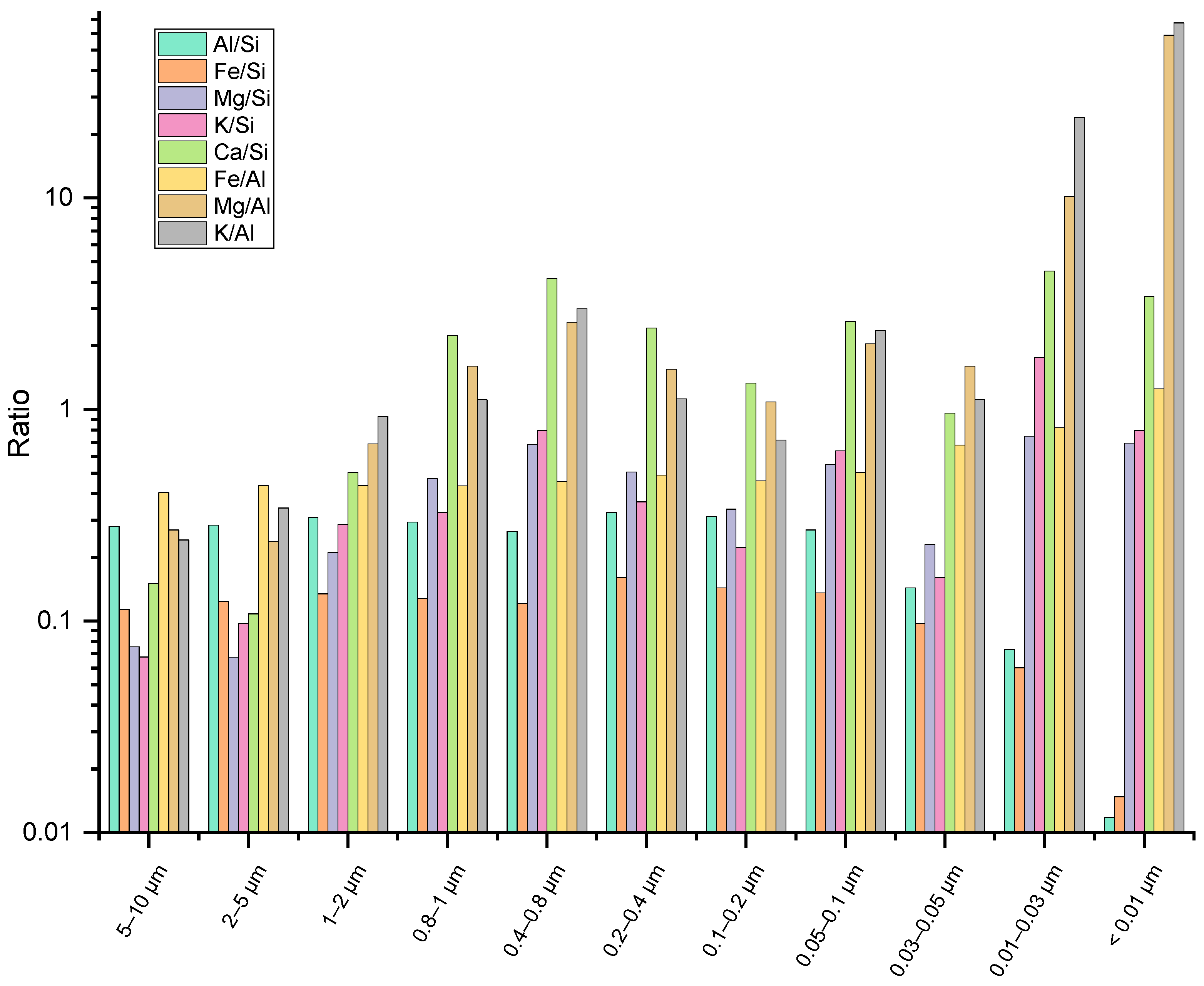
4.6. Molar Ratios of Major Elements

The existing data indicate that labile aluminosilicates predominate in the mineralogical composition of the silty fraction of below 1 µm of the similar Kursk chernozem, except for the arable land [16]. In the fraction below 0.2 µm, about 25% of kaolinite and chlorite, about 53% of illites, and about 22% of labile silicates (montmorillonite) were found. In the fraction of 0.2–1 µm, the contents of kaolinite and chlorites were ca. 57%; illites, 35%; and labile silicates, 8%. In coarse fractions of 1–10 µm, quartz predominates; clay minerals were distributed as follows: 38% kaolinite and chlorites, 50% illites, 12% labile silicates [16]. It is noteworthy that with regular plowing and under the influence of mineral fertilizers, clay minerals are decomposed and removed, and the content of dust fractions and quartz in them increases [50,51,52,53]. Therefore, we only consider these ratios as an example.

According to the accepted formulas of the chemical composition of kaolinite minerals Si₄Al₄O₁₀(OH)₈, montmorillonite (Na,Ca)_0,33(Al,Mg)₂Si₄O₁₀(OH)₂(H₂O)_n, and illite (K,H₃O)(Al,Mg,Fe)₂(Si,Al)₄(H₂O) [54], the molar ratio of Al/Si in kaolinite should be ca. 1; in montmorillonite it should be 0.25–0.5 (the same for Mg/Si); and in illite it should be 1.0–1.5. The Mg/Al ratio in montmorillonite is ca. 1; in illite, it is ca. 0.2. In our case, for large fractions of 5–10 and 2–5 µm, the calculated ratios do not change, which indicates the homogeneity of their mineralogical composition and its predominantly silicate nature with a uniform distribution of smectite-like (montmorillonite-like) and illite-like structures, most likely mixed-layered. In WESC fractions decreasing from 1 to 0.05 µm, the relative content increased 2–4-fold for K and Mg and 8-fold for Ca (Figure 7), with almost unchanged ratios of Al/Si, Fe/Si, and Fe/Al (Figure 8). This may indicate predominant clay minerals and carbonates in the composition of these fractions. The distribution of hydrates of aluminum and iron oxides can be traced by the ratios of Fe/Al, Fe/Si, and Al/Si, which almost do not change in fractions of 0.05–10 µm. Thus, it suggests approximately the same level of mineral contents, apparently existing in the form of films covering individual particles of clay minerals, possibly in combination with organic matter. In the fraction of 0.01–0.03 µm, all ratios change considerably, which indicates the predominance of non-silicate compounds of iron and aluminum, as well as other macroelements. The fraction of below 0.01 µm almost does not contain aluminosilicates; the elements are found in other water-soluble forms. The isolated fraction of 0.03–-0.05 µm could be considered transitional. Apparently, the boundary of the transition of the existence of crystallized and non-crystallized forms of clay minerals lies at a level of ca. 0.02 µm. The obtained data on the forms of existence of macroelements correspond to the particle sizes of non-silicate minerals: Fe, up to 17–22 nm; Mn and Ti oxides, up to 6–12 nm; and amorphous SiO₂, up to 12 nm [55,56].

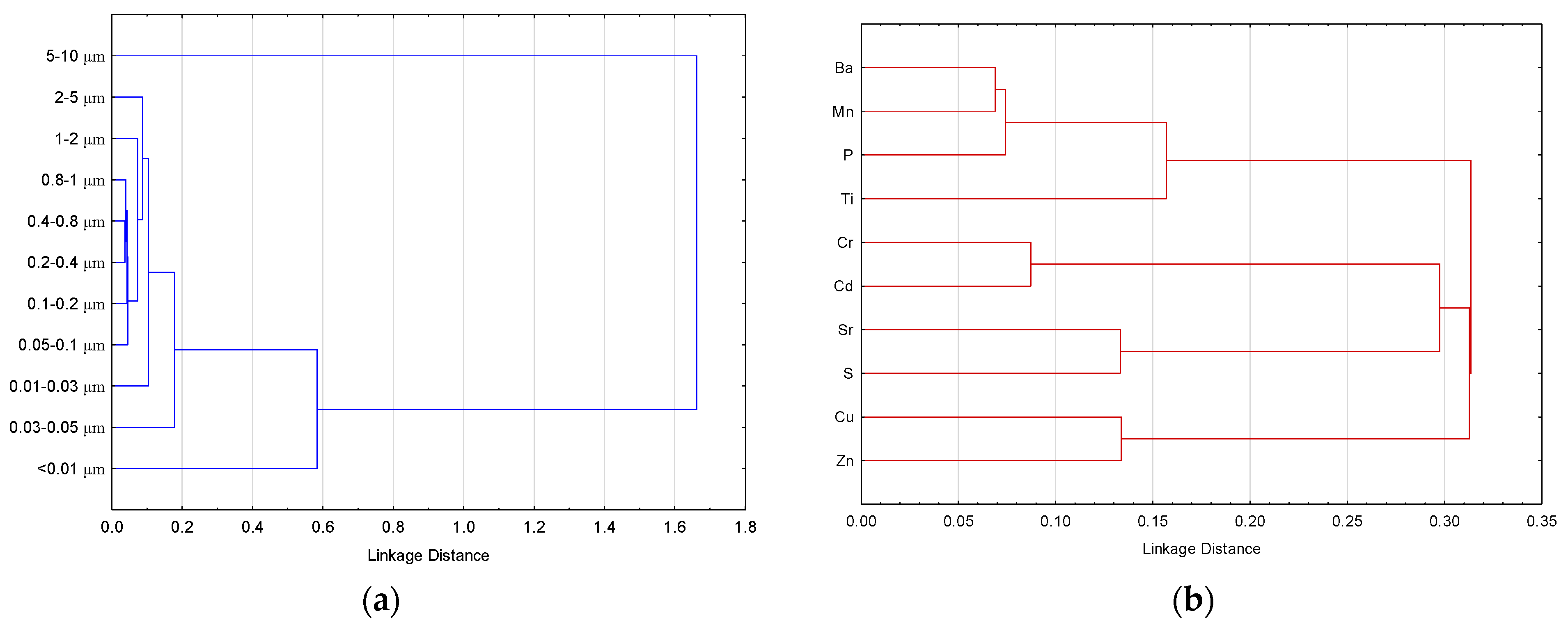
4.7. Cluster Analysis and Modeling of Element Distributions

Analysis of the distribution of the entire set of macro- and microelements shows that the size groups of particles of 2–5, 1–2, and 0.05–0.1 µm and a set of other size fractions, including below 0.01 µm, are clustered according to the content levels (Figure 11a). The grouping of elements is as follows: Ca, Si, and the rest of elements are fundamentally separated, consisting of both groups associated with the silicate matrix and forming non-silicate mineral phases (Figure 11b). In the following subsections, we consider the distributions of the main elements that form silicate and ferruginous mineral phases.

4.7.1. Distribution of Main Elements

As noted above, the composition of soil colloids is heterogeneous. Their inorganic part mainly consists of microparticles of clay aluminosilicates of varying degrees of crystallinity and minerals, hydrates of iron, and aluminum oxides [57]. The main structure-forming elements are Si, Al, Fe, Mg, K, and Na. In terms of elemental composition, clustering occurs at the level of size fractions and sums (groups) of fractions of 5–10, 1–5, 0.03–1, and below 0.01 µm (Figure 12a).

4.7.2. Medium- and Low-Concentration Elements

Two large groups are found that correlate with the above sets: Si + (Al + Fe) and (Mg + K) + Ca (Figure 12b). These two large clusters are associated with the anionic and cationic parts of aluminosilicates. The separation within the anionic–cationic first and cationic second isolated groups is due to the existence of these elements both in the form of aluminosilicates and non-silicate minerals, hydrates of iron and aluminum oxides, and carbonates, mainly calcium. It is contained in carbonates, while Fe and Al exist in the forms of non-silicate minerals.

In terms of elemental composition, clustering for the related elements of Sets 1–4 (Ba, Cd, Cr, Cu, Mn, Sr, Ti, Zn, P, and S) is similar to that for the main elements of fractions of 5–10 and below 0.01 µm. Between these fractions, there are combined fractions from 1 to 5 µm, 0.05–1 µm, and 0.01–0.05 µm (compare Figure 12a and Figure 13a). The nature of the distribution of other elements is different, which is associated with the species in the soil mainly being metal organic complexes or other coordination compounds and sorbed labile aluminosilicates and non-silicate ferruginous minerals. It is obvious that the largest fractions, consisting of microaggregated organo-clay particles, contain all the identified elements in a variety of their natural forms. The smallest fractions predominantly contain nanoparticles with sorbed non-silicate iron minerals (as well as chromium and manganese), low molecular weight water-soluble organic substances, and calcium and magnesium carbonates.

There are three main groups of elements, Ba + Mn + P; Ti and (Cr + Cd; Sr + S); and (Cu + Zn) (Figure 13b), that correspond to the concept of the mineral species of these elements in soils [58]. It is known that Ba is associated with sulfates and carbonates and is concentrated in minerals and nodules containing Mn and P (Figure 13b). The main part of Ba is in particles of 0.4–0.8 µm and is not confined to either aluminosilicates or organometallic compounds, which reflects its position in Figure 9 almost in the central position. Titanium concentrations are extremely low, and TiO₂ particle sizes are below 15 nm, corresponding to those of the main ferrous minerals [56]; however, the nature of its distribution in the obtained fractions, with a pronounced accumulation in large particles, is similar to the nature of the distribution of iron and aluminum, as illustrated by Figure 9. In this case, cadmium is associated with chromium, which usually exists in the composition of ferruginous non-silicate minerals (Figure 9 and Figure 12b) known as being cadmium sorbents. Cu and Zn appear to be associated with the living matter of soils [58] and are present in aqueous extracts as coordination compounds with organic matter.

The composition of cations in the finest fractions (sizes below 0.1 µm) that contain almost no already crystallized silicate minerals is determined by the processes of precipitation–dissolution and ion exchange processes. The role of the main soil components—layered clay aluminosilicate minerals and non-silicate minerals of iron and manganese oxide hydrates with a highly developed specific surface area, and soil organic matter—in the formation of the agro-ecological and toxicological state of soils and their buffering capacity has been studied for many decades and continues to be researched [59,60,61,62,63,64].

Since studies of separated fractions of aqueous extractions from soils have not been carried out, the results obtained in this study can be compared with those that describe the composition and content of elements in water extracts in general, as well as in soil and groundwater; waters of coastal sea, river, and lake areas; and in the composition of bottom sediments. Such studies have been carried out for many years; the interest in them was high in the last third of the 20th century. This is confirmed by the well-known monograph by G. Sposito [65] as well as other studies by this author [66]. According to [67], high contents of Cr, Fe, Cu, Zn, and Pb in marine bottom sediments are the result of inputs with non-silicate iron (hydro)oxide minerals and carbonate mineral phases, and phase redistribution can occur in the zones mixing fresh- and seawater in the estuarine zone. The predominant contribution of iron–manganese minerals to the migration of heavy metals to marine environments is mentioned [68]. Soil salinization also affects the migratory capacity of heavy metals by changing the ionic strength of the soil solution, pH, and redox potential, which determines the state of iron–manganese minerals [69]. The influence of environmental acidity, caused, apart from natural processes, by industrial acid emissions, can be compensated by the mineralogical and granulometric heterogeneity of soils [70].

Although many studies have established that major potentially hazardous elements such as lead, cadmium, zinc, copper, and arsenic in areas of anthropogenic contamination can be largely associated with non-silicate ferruginous and, indirectly, layered clay minerals [71], this study confirms the previous data [72,73]; native studies of the spatial distributions of elements show that the finest fraction is able to migrate both vertically and laterally with the flow of water during periods of increased humidity. The preferential migration of elements in fractions of clusters of different size is also described in approaches with the comparison of the fractal content in the development of the approach by G. Sposito [66], which combines broad size ranges starting with the smallest particles of 0.2 µm [74]. These studies clearly show the preferential differentiation of the element composition in connection with the size differentiation of soil particles. The relationship between the mineralogical composition of fine fractions and the migratory ability of a number of elements in terms of their recoverability as exchangeable species was also clearly demonstrated [67].

At the level of macroaggregates, such studies are also actively carried out to assess the safety of soils in agricultural production [75]. The highest content of heavy metals was found in the smallest aggregates; it decreases with increasing aggregate size [75]. Correlation analysis showed that the distribution of the minerals of Fe and Mn and total organic carbon have a significant impact on the distribution of Pb, Cd, As, and Cr. These data are consistent with our findings.

5. Conclusions

In this study, we proposed a methodology for the fractionation of particulate soil organic matter (WESC) for a wide range of particles using analytical track-etched membranes, which is a logical continuation of cascade sieve fractionation for larger size fractions. This method provides the separation and isolation of particles with a size of less than 10 µm down to 10 nm. For a more complete profiling of WESCs from the viewpoint of SOM, studies of soil colloids with molecular spectroscopy methods (UV/vis, FTIR, and fluorescence spectroscopy) should also be involved. However, based on the findings of this study, it is possible to evaluate the advantages and disadvantages of the proposed approach. The pros are the technical simplicity and relatively low cost of such separations available for almost any laboratory. Also, the advantages include a wide selection of filter materials, their sizes, and suppliers.

At the same time, the shortcomings of the approach are primarily its high labor and time costs, e.g., filtering fractions through membranes with pores smaller than 0.05 µm took hours, which is completely unacceptable for the analysis of many samples, typical for screening studies. Thus, to scale the approach, it is necessary to design a cascade device and shift from vacuum to pressure filtration. There is also the problem of clogging the pores of membrane filters during the filtration process. In this work, this problem was solved by frequent replacement of filters (up to ten filters per fraction, typically three to five), which leads to their increased consumption. It is necessary to optimize the number of consumable filters and assess the degree of pore-clogging.

From the viewpoint of element analysis of water-extractable soil colloids, a set of narrow size fractions provides detailed element soil profiles for such fine fractions. This was facilitated by the reliable methodology of ICP–AES. This profiling reveals rather distinct differences and the individual character of each fraction as well as trends in the changes in the mineral matrix of WESCs and microelement composition with fraction size. Si, Al, Fe, and Ti are accumulated (as absolute concentrations and percentages) in fractions with sizes above 1 µm, while Ca, Mg, Mn, Cu, Zn, K, and S are accumulated in fractions below 1 µm.

Thus, we consider the proposed approach based on ultrafiltration with track-etched membranes promising and believe it is important to further develop it as part of the methodology for the complex analysis of soil organic matter. The proposed approach expands knowledge on the element composition of organo-clay colloidal soil particles.

References

1. Chantigny, M.H.; Angers, D.A.; Kaiser, K.; Kalbitz, K. Extraction and characterization of dissolved organic matter. In Soil Sampling and Methods of Analysis; Carter, M.R., Gregorich, E.G., Eds.; CRC Press: Boca Raton, FL, USA, 2007. [Google Scholar]
2. Aiken, G.R.; Hsu-Kim, H.; Ryan, J.N. Influence of dissolved organic matter on the environmental fate of metals, nanoparticles, and colloids. Environ. Sci. Technol. 2011, 45, 3196–3201. [Google Scholar] [CrossRef]
3. Hendricks, S.B.; Fry, W.H. The Results of X-Ray and Microscopical Examinations of Soil Colloids. Soil Sci. Soc. Am. J. 1930, B11, 194–195. [Google Scholar] [CrossRef]
4. Osman, K.T. Chemical Properties of Soil. In Soils: Principles, Properties and Management; Springer: Dordrecht, The Netherlands, 2013; pp. 97–111. [Google Scholar]
5. Yang, W.; Bradford, S.A.; Wang, Y.; Sharma, P.; Shang, J.; Li, B. Transport of biochar colloids in saturated porous media in the presence of humic substances or proteins. Environ. Pollut. 2019, 246, 855–863. [Google Scholar] [CrossRef]
6. Ranville, J.F.; Chittleborough, D.J.; Beckett, R. Particle-Size and Element Distributions of Soil Colloids. Soil Sci. Soc. Am. J. 2005, 69, 1173–1184. [Google Scholar] [CrossRef]
7. Wei, Z.; Zhu, Y.; Wang, Y.; Song, Z.; Wu, Y.; Ma, W.; Hou, Y.; Zhang, W.; Yang, Y. Influence of Soil Colloids on Ni Adsorption and Transport in the Saturated Porous Media: Effects of pH, Ionic Strength, and Humic Acid. Appl. Sci. 2022, 12, 6591. [Google Scholar] [CrossRef]
8. Li, C.; Guo, S. Structural evolution of soil aggregates in a karst rocky desertification area. RSC Adv. 2022, 12, 21004–21013. [Google Scholar] [CrossRef]
9. Pan, Y.; Chen, C.; Shang, J. Effect of reduced inherent organic matter on stability and transport behaviors of black soil colloids. Chemosphere 2023, 336, 139149. [Google Scholar] [CrossRef]
10. Moens, C.; Dondeyne, S.; Panagea, I.; Smolders, E. Depth profile of colloidal iron in the pore water of an Albic Podzol. Eur. J. Soil Sci. 2022, 73, e13305. [Google Scholar] [CrossRef]
11. Witzgall, K.; Vidal, A.; Schubert, D.I.; Hoschen, C.; Schweizer, S.A.; Buegger, F.; Pouteau, V.; Chenu, C.; Mueller, C.W. Particulate organic matter as a functional soil component for persistent soil organic carbon. Nat. Commun. 2021, 12, 4115. [Google Scholar] [CrossRef]
12. Li, S.; Chen, S.; Bai, S.; Tan, J.; Jiang, X. Intensive agricultural management-induced subsurface accumulation of water extractable colloidal P in lime concretion black soil. EGUsphere 2023, 2023, 1–24. [Google Scholar] [CrossRef]
13. Cheng, T.; Saiers, J.E. Effects of dissolved organic matter on the co-transport of mineral colloids and sorptive contaminants. J. Contam. Hydrol. 2015, 177–178, 148–157. [Google Scholar] [CrossRef] [PubMed]
14. Chen, J.; Zhang, H.; Wei, Q.; Farooq, U.; Zhang, Q.; Lu, T.; Wang, X.; Chen, W.; Qi, Z. Mobility of water-soluble aerosol organic matters (WSAOMs) and their effects on soil colloid-mediated transport of heavy metal ions in saturated porous media. J. Hazard. Mater. 2022, 440, 129733. [Google Scholar] [CrossRef] [PubMed]
15. Zhou, D.; Liang, M.; Bao, X.; Sun, T.; Huang, Y. Effects of soil colloids on the aggregation and degradation of engineered nanoparticles (Ti(3)C(2)T(x) MXene). Environ. Res. 2022, 214, 113886. [Google Scholar] [CrossRef] [PubMed]
16. Petrofanov, V.L. Role of the soil particle-size fractions in the sorption and desorption of potassium. Eurasian Soil Sci. 2012, 45, 598–611. [Google Scholar] [CrossRef]
17. Swift, R.S.; McLaren, R.G. Micronutrient Adsorption by Soils and Soil Colloids. In Interactions at the Soil Colloid—Soil Solution Interface; Bolt, G.H., De Boodt, M.F., Hayes, M.H.B., McBride, M.B., De Strooper, E.B.A., Eds.; Springer: Dordrecht, The Netherlands, 1991; pp. 257–292. [Google Scholar]
18. Molina, F.V. Soil Colloids, 1st ed.; CRC Press: Boca Raton, FL, USA, 2016. [Google Scholar]
19. Lead, J.R.; Wilkinson, K.J. Environmental Colloids and Particles: Current Knowledge and Future Developments. In Environmental Colloids and Particles; Wiley: Chichester, UK, 2007; pp. 1–15. [Google Scholar]
20. Schluter, S.; Leuther, F.; Albrecht, L.; Hoeschen, C.; Kilian, R.; Surey, R.; Mikutta, R.; Kaiser, K.; Mueller, C.W.; Vogel, H.J. Microscale carbon distribution around pores and particulate organic matter varies with soil moisture regime. Nat. Commun. 2022, 13, 2098. [Google Scholar] [CrossRef]
21. Devitt, E.C.; Wiesner, M.R. Dialysis Investigations of Atrazine-Organic Matter Interactions and the Role of a Divalent Metal. Environ. Sci. Technol. 1998, 32, 232–237. [Google Scholar] [CrossRef]
22. Jansen, B.; Kotte, M.C.; van Wijk, A.J.; Verstraten, J.M. Comparison of diffusive gradients in thin films and equilibrium dialysis for the determination of Al, Fe(III) and Zn complexed with dissolved organic matter. Sci. Total Environ. 2001, 277, 45–55. [Google Scholar] [CrossRef]
23. Pan, Y.; Li, H.; Zhang, X.; Li, A. Characterization of natural organic matter in drinking water: Sample preparation and analytical approaches. Trends Environ. Anal. Chem. 2016, 12, 23–30. [Google Scholar] [CrossRef]
24. Brezinski, K.; Gorczyca, B. An overview of the uses of high performance size exclusion chromatography (HPSEC) in the characterization of natural organic matter (NOM) in potable water, and ion-exchange applications. Chemosphere 2019, 217, 122–139. [Google Scholar] [CrossRef]
25. Picó, Y.; Barceló, D. Pyrolysis gas chromatography-mass spectrometry in environmental analysis: Focus on organic matter and microplastics. TrAC Trends Anal. Chem. 2020, 130, 115964. [Google Scholar] [CrossRef]
26. Volkov, D.; Rogova, O.; Proskurnin, M. Organic Matter and Mineral Composition of Silicate Soils: FTIR Comparison Study by Photoacoustic, Diffuse Reflectance, and Attenuated Total Reflection Modalities. Agronomy 2021, 11, 1879. [Google Scholar] [CrossRef]
27. Quinn, J.A.; Anderson, J.L.; Ho, W.S.; Petzny, W.J. Model pores of molecular dimension. The preparation and characterization of track-etched membranes. Biophys. J. 1972, 12, 990–1007. [Google Scholar] [CrossRef] [PubMed]
28. Chakarvarti, S.K. Track-etch membranes enabled nano-/microtechnology: A review. Radiat. Meas. 2009, 44, 1085–1092. [Google Scholar] [CrossRef]
29. Brink, L.E.S.; Elbers, S.J.G.; Robbertsen, T.; Both, P. The anti-fouling action of polymers preadsorbed on ultrafiltration and microfiltration membranes. J. Membr. Sci. 1993, 76, 281–291. [Google Scholar] [CrossRef]
30. Yamazaki, I.M.; Paterson, R.; Geraldo, L.P. A new generation of track etched membranes for microfiltration and ultrafiltration. Part I. Preparation and characterisation. J. Membr. Sci. 1996, 118, 239–245. [Google Scholar] [CrossRef]
31. Croue, J.-P.; Korshin, G.V.; Benjamin, M.M. Characterization of Natural Organic Matter in Drinking Water; American Water Works Association, AwwRF: Denver, CO, USA, 2000. [Google Scholar]
32. Minor, E.C.; Swenson, M.M.; Mattson, B.M.; Oyler, A.R. Structural characterization of dissolved organic matter: A review of current techniques for isolation and analysis. Environ. Sci. Process Impacts 2014, 16, 2064–2079. [Google Scholar] [CrossRef]
33. Sillanpää, M.; Metsämuuronen, S.; Mänttäri, M. Membranes. In Natural Organic Matter in Water; Sillanpää, M., Ed.; Butterworth-Heinemann: Oxford, UK, 2015; pp. 113–157. [Google Scholar]
34. Ben-Sasson, M.; Zidon, Y.; Calvo, R.; Adin, A. Enhanced removal of natural organic matter by hybrid process of electrocoagulation and dead-end microfiltration. Chem. Eng. J. 2013, 232, 338–345. [Google Scholar] [CrossRef]
35. Proskurnin, M.A.; Volkov, D.S.; Rogova, O.B. Two-Dimensional Correlation IR Spectroscopy of Humic Substances of Chernozem Size Fractions of Different Land Use. Agronomy 2023, 13, 1696. [Google Scholar] [CrossRef]
36. Volkov, D.S.; Rogova, O.B.; Proskurnin, M.A.; Farkhodov, Y.R.; Markeeva, L.B. Thermal stability of organic matter of typical chernozems under different land uses. Soil Tillage Res. 2020, 197, 104500. [Google Scholar] [CrossRef]
37. Chantigny, M.H.; Harrison-Kirk, T.; Curtin, D.; Beare, M. Temperature and duration of extraction affect the biochemical composition of soil water-extractable organic matter. Soil Biol. Biochem. 2014, 75, 161–166. [Google Scholar] [CrossRef]
38. Zsolnay, Á. Chapter 4—Dissolved Humus in Soil Waters. In Humic Substances in Terrestrial Ecosystems; Piccolo, A., Ed.; Elsevier Science B.V.: Amsterdam, The Netherlands, 1996; pp. 171–223. [Google Scholar]
39. Waller, P.A.; Pickering, W.F. The lability of copper ions sorbed on humic acid. Chem. Speciat. Bioavailab. 1990, 2, 127–138. [Google Scholar] [CrossRef]
40. Stevenson, F.J.; Chen, Y. Stability Constants of Copper(II)-Humate Complexes Determined by Modified Potentiometric Titration. Soil Sci. Soc. Am. J. 1991, 55, 1586–1591. [Google Scholar] [CrossRef]
41. Boguta, P.; Sokołowska, Z. Interactions of Zn(II) Ions with Humic Acids Isolated from Various Type of Soils. Effect of pH, Zn Concentrations and Humic Acids Chemical Properties. PLoS ONE 2016, 11, e0153626. [Google Scholar] [CrossRef] [PubMed]
42. Piotrowicz, S.R.; Harvey, G.R.; Boran, D.A.; Weisel, C.P.; Springer-Young, M. Cadmium, copper, and zinc interactions with marine humus as a function of ligand structure. Mar. Chem. 1984, 14, 333–346. [Google Scholar] [CrossRef]
43. Lyvén, B.; Hassellöv, M.; Turner, D.R.; Haraldsson, C.; Andersson, K. Competition between iron- and carbon-based colloidal carriers for trace metals in a freshwater assessed using flow field-flow fractionation coupled to ICPMS. Geochim. Cosmochim. Acta 2003, 67, 3791–3802. [Google Scholar] [CrossRef]
44. Sokolova, T.A.; Zaidel’man, F.R.; Ginzburg, T.M. Clay minerals in chernozem-like soils of mesodepressions in the northern forest-steppe of European Russia. Eurasian Soil Sci. 2010, 43, 76–84. [Google Scholar] [CrossRef]
45. Goldberg, S. Interaction of aluminum and iron oxides and clay minerals and their effect on soil physical properties: A review. Commun. Soil Sci. Plant Anal. 1989, 20, 1181–1207. [Google Scholar] [CrossRef]
46. Krivoshein, P.K.; Volkov, D.S.; Rogova, O.B.; Proskurnin, M.A. FTIR photoacoustic spectroscopy for identification and assessment of soil components: Chernozems and their size fractions. Photoacoustics 2020, 18, 100162. [Google Scholar] [CrossRef]
47. Mitrović, B.; Milačič, R. Speciation of aluminium in forest soil extracts by size exclusion chromatography with UV and ICP-AES detection and cation exchange fast protein liquid chromatography with ETAAS detection. Sci. Total Environ. 2000, 258, 183–194. [Google Scholar] [CrossRef]
48. Milnes, A.R.; Fitzpatrick, R.W. Titanium and Zirconium Minerals. In Minerals in Soil Environments, 2nd ed.; Dixon, J.B., Weed, S.B., Eds.; Soil Science America: Madison, WI, USA, 1989; Volume 1. [Google Scholar]
49. Schulze, D.G. An Introduction to Soil Mineralogy. In Minerals in Soil Environments, 2nd ed.; Dixon, J.B., Weed, S.B., Eds.; Soil Science America: Madison, WI, USA, 1989; Volume 1. [Google Scholar]
50. Barré, P.; Velde, B.; Abbadie, L. Dynamic role of “illite-like” clay minerals in temperate soils: Facts and hypotheses. Biogeochemistry 2006, 82, 77–88. [Google Scholar] [CrossRef]
51. Bühmann, C.; Beukes, D.J.; Turner, D.P. Clay mineral associations in soils of the Lusikisiki area, Eastern Cape Province, and their agricultural significance. S. Afr. J. Plant Soil 2006, 23, 78–86. [Google Scholar] [CrossRef]
52. Tao, L.; Wen, X.; Li, H.; Huang, C.; Jiang, Y.; Liu, D.; Sun, B. Influence of manure fertilization on soil phosphorous retention and clay mineral transformation: Evidence from a 16-year long-term fertilization experiment. Appl. Clay Sci. 2021, 204, 106021. [Google Scholar] [CrossRef]
53. Simonsson, M.; Hillier, S.; Öborn, I. Changes in clay minerals and potassium fixation capacity as a result of release and fixation of potassium in long-term field experiments. Geoderma 2009, 151, 109–120. [Google Scholar] [CrossRef]
54. Kumari, N.; Mohan, C. Basics of Clay Minerals and Their Characteristic Properties. In Clay and Clay Minerals; Gustavo Morari Do, N., Ed.; IntechOpen: Rijeka, Croatia, 2021; p. 2. [Google Scholar]
55. Goldberg, S.R.; Lebron, I.; Seaman, J.C.; Suarez, D.L. Soil colloidal behavior. In Handbook of Soil Sciences Properties and Processes, 2nd ed.; Huang, P.M., Li, Y., Sumner, M.E., Eds.; CRC Press: Boca Raton, FL, USA; Taylor and Francis Group: Abingdon, UK, 2012; pp. 15-11–15-39. [Google Scholar]
56. Davis, J.A.; Kent, D.B. Surface complexation modeling in aqueous geochemistry. Rev. Mineral. Geochem. 1990, 23, 177–260. [Google Scholar]
57. Beamlaku, A.; Habtemariam, T. Soil Colloids, Types and their Properties: A review. Open J. Bioinform. Biostat. 2021, 5, 008–113. [Google Scholar] [CrossRef]
58. Kabata-Pendias, A. Trace Elements in Soils and Plants, 4th ed.; CRC Press: Boca Raton, FL, USA, 2010. [Google Scholar]
59. Sposito, G. Derivation of the Freundlich Equation for Ion Exchange Reactions in Soils. Soil Sci. Soc. Am. J. 1980, 44, 652–654. [Google Scholar] [CrossRef]
60. Lair, G.J.; Gerzabek, M.H.; Haberhauer, G. Sorption of heavy metals on organic and inorganic soil constituents. Environ. Chem. Lett. 2006, 5, 23–27. [Google Scholar] [CrossRef]
61. Covelo, E.F.; Vega, F.A.; Andrade, M.L. Competitive sorption and desorption of heavy metals by individual soil components. J. Hazard. Mater. 2007, 140, 308–315. [Google Scholar] [CrossRef]
62. Golia, E.E.; Kantzou, O.-D.; Chartodiplomenou, M.-A.; Papadimou, S.G.; Tsiropoulos, N.G. Study of Potentially Toxic Metal Adsorption in a Polluted Acid and Alkaline Soil: Influence of Soil Properties and Levels of Metal Concentration. Soil Syst. 2023, 7, 16. [Google Scholar] [CrossRef]
63. Nikishina, M.; Perelomov, L.; Atroshchenko, Y.; Ivanova, E.; Mukhtorov, L.; Tolstoy, P. Sorption of Fulvic Acids and Their Compounds with Heavy Metal Ions on Clay Minerals. Soil Syst. 2022, 6, 2. [Google Scholar] [CrossRef]
64. Shaheen, S.M.; Derbalah, A.S.; Moghanm, F.S. Removal of Heavy Metals from Aqueous Solution by Zeolite in Competitive Sorption System. Int. J. Environ. Sci. Dev. 2012, 3, 362–367. [Google Scholar] [CrossRef]
65. Sposito, G. The Thermodynamics of Soil Solutions; Oxford University Press: Oxford, UK, 1981. [Google Scholar]
66. Rieu, M.; Sposito, G. Fractal Fragmentation, Soil Porosity, and Soil Water Properties: I. Theory. Soil Sci. Soc. Am. J. 1991, 55, 1231–1238. [Google Scholar] [CrossRef]
67. Tokar’, E.; Kuzmenkova, N.; Rozhkova, A.; Egorin, A.; Shlyk, D.; Shi, K.; Hou, X.; Kalmykov, S. Migration Features and Regularities of Heavy Metals Transformation in Fresh and Marine Ecosystems (Peter the Great Bay and Lake Khanka). Water 2023, 15, 2267. [Google Scholar] [CrossRef]
68. Ling, S.Y.; Asis, J.; Musta, B. Distribution of metals in coastal sediment from northwest sabah, Malaysia. Heliyon 2023, 9, e13271. [Google Scholar] [CrossRef]
69. Sheng, W.; Hou, Q.; Yang, Z.; Yu, T. Impacts of periodic saltwater inundation on heavy metals in soils from the Pearl River Delta, China. Mar. Environ. Res. 2023, 187, 105968. [Google Scholar] [CrossRef] [PubMed]
70. Qi, S.; Li, X.; Luo, J.; Han, R.; Chen, Q.; Shen, D.; Shentu, J. Soil heterogeneity influence on the distribution of heavy metals in soil during acid rain infiltration: Experimental and numerical modeling. J. Environ. Manag. 2022, 322, 116144. [Google Scholar] [CrossRef]
71. Ke, W.; Zeng, J.; Zhu, F.; Luo, X.; Feng, J.; He, J.; Xue, S. Geochemical partitioning and spatial distribution of heavy metals in soils contaminated by lead smelting. Environ. Pollut. 2022, 307, 119486. [Google Scholar] [CrossRef]
72. Anaman, R.; Peng, C.; Jiang, Z.; Liu, X.; Zhou, Z.; Guo, Z.; Xiao, X. Identifying sources and transport routes of heavy metals in soil with different land uses around a smelting site by GIS based PCA and PMF. Sci. Total Environ. 2022, 823, 153759. [Google Scholar] [CrossRef]
73. Zeng, J.; Tabelin, C.B.; Gao, W.; Tang, L.; Luo, X.; Ke, W.; Jiang, J.; Xue, S. Heterogeneous distributions of heavy metals in the soil-groundwater system empowers the knowledge of the pollution migration at a smelting site. Chem. Eng. J. 2023, 454, 140307. [Google Scholar] [CrossRef]
74. Tian, Z.; Pan, Y.; Chen, M.; Zhang, S.; Chen, Y. The relationships between fractal parameters of soil particle size and heavy-metal content on alluvial-proluvial fan. J. Contam. Hydrol. 2023, 254, 104140. [Google Scholar] [CrossRef]
75. Gong, C.; Shao, Y.; Luo, M.; Xu, D.; Ma, L. Distribution Characteristics of Heavy Metals in Different Particle Size Fractions of Chinese Paddy Soil Aggregates. Processes 2023, 11, 1873. [Google Scholar] [CrossRef]
Figure 1. Sequential membrane fractionation system.
Agrochemicals 02 00032 g001
Figure 2. Correlation map of determined elements (except Na) for polycarbonate cold extracts after membrane fractionation for all size fractions.
Agrochemicals 02 00032 g002
Figure 3. Distribution of elements of Set 1 in polycarbonate cold extracts. Relative standard deviation for the elements except iron is no more than 2%; for iron, no more than 4%.
Agrochemicals 02 00032 g003
Figure 4. Distribution of elements of Set 2 in polycarbonate cold extracts. Relative standard deviation for the elements is no more than 0.5%.
Agrochemicals 02 00032 g004
Figure 5. Distribution of elements of Set 3 in polycarbonate cold extracts. Relative standard deviation for the elements is no more than 0.5%.
Agrochemicals 02 00032 g005
Figure 6. Distribution of elements of Set 4 in polycarbonate cold extracts. Relative standard deviation for the elements is no more than 0.5%.
Agrochemicals 02 00032 g006
Figure 7. Whole element distribution as average mass percentage for polycarbonate cold extracts on the particle size.
Agrochemicals 02 00032 g007
Figure 8. Average molar ratios of major elements in extracts on the particle size.
Agrochemicals 02 00032 g008
Figure 9. Factor analysis of distribution of all the elements. Factor 1, from bottom to top, an increase in the biogenicity of elements; Factor 2, from left to right, an increase in the particle size.
Agrochemicals 02 00032 g009
Figure 10. Total amounts of elements for polycarbonate cold extracts on the particle size. Relative standard deviation for the elements is no more than 2%.
Agrochemicals 02 00032 g010
Figure 11. Cluster analysis (single linkage, Euclidean distances) of the contents of the entire set of elements (mol/kg); (a) cases, fraction sizes and (b) variables, elements.
Agrochemicals 02 00032 g011
Figure 12. Cluster analysis (single linkage, Euclidean distances) of the distribution of the main mineral-forming macroelements (mol/kg); (a) cases, fraction sizes and (b) variables, elements.
Agrochemicals 02 00032 g012
Figure 13. Cluster analysis (single linage, Euclidean distances) of the share distribution of medium- and low-concentration elements (mol/kg); (a) cases, fraction sizes and (b) variables, elements.
Agrochemicals 02 00032 g013