
Oil Prices, World Trade Policy Uncertainty, and the Trade Balance: The Case of Korea


Department of Economics, College of Business and Security Management, University of Alaska, Fairbanks, AK 99775, USA
Commodities 2023, 2(3), 188-200; https://doi.org/10.3390/commodities2030012
Submission received: 28 March 2023
/
Revised: 3 June 2023
/
Accepted: 15 June 2023
/
Published: 26 June 2023
(This article belongs to the Special Issue Uncertainty, Economic Risk and Commodities Markets)
Abstract
:This article studies the asymmetric effects that the price of crude oil has on Korean exports to and imports from its largest partners—China, the U.S., and Japan—controlling for world trade policy uncertainty. The results support the evidence of the long-run asymmetry of oil prices for Korea’s exports to Japan, and imports from China and Japan. However, there is no evidence of the short-run asymmetry of oil prices. Finally, world trade policy uncertainty appears to be more important for determining Korea’s bilateral trade in the short run than in the long run.
1. Introduction
Over the past decades, many authors have attempted to explain how oil prices influence the balance of trade. The prevailing findings regarding the subject indicate that net oil importers experience terms-of-trade effects. These effects suggest that higher (lower) oil prices tend to reduce (increase) exports in net oil importers due to an increase (decrease) in production costs, leading to a deterioration (improvement) in trade balance. Another extensively acknowledged aspect is the potential revenue effects experienced by net oil exporters. This concept posits that increases (declines) in oil prices are likely to stimulate (reduce) the export of crude oil from oil-producing nations, consequently boosting (lowering) oil revenues and leading to a trade surplus (deficit). Undeniably, prior studies have significantly contributed to enhancing our knowledge and comprehension of how a country’s trade balance responds to oil price shocks.
However, earlier studies have some serious weaknesses. First, previous studies typically concentrate on the compilation of trade balances of multiple countries in light of a two-country model—between a country and the rest of the world. Given that a country could improve the trade balance with one partner while simultaneously deteriorating it with another, the use of aggregate trade data is likely to cause aggregation bias of data. Second, since the composition and pattern of a country’s exports and imports are bound to be different, analyzing the trade balance measured in trade surplus or deficit of an economy in a model is not able to properly uncover the oil price impacts on exports and imports, thereby generating misleading outcomes. The third shortcoming is that, although world trade policy uncertainty negatively affects global economic activity through a reduction in investment and employment, thereby shrinking international trade flow, little emphasis has been given to the trade uncertainty impact when tackling the subject.
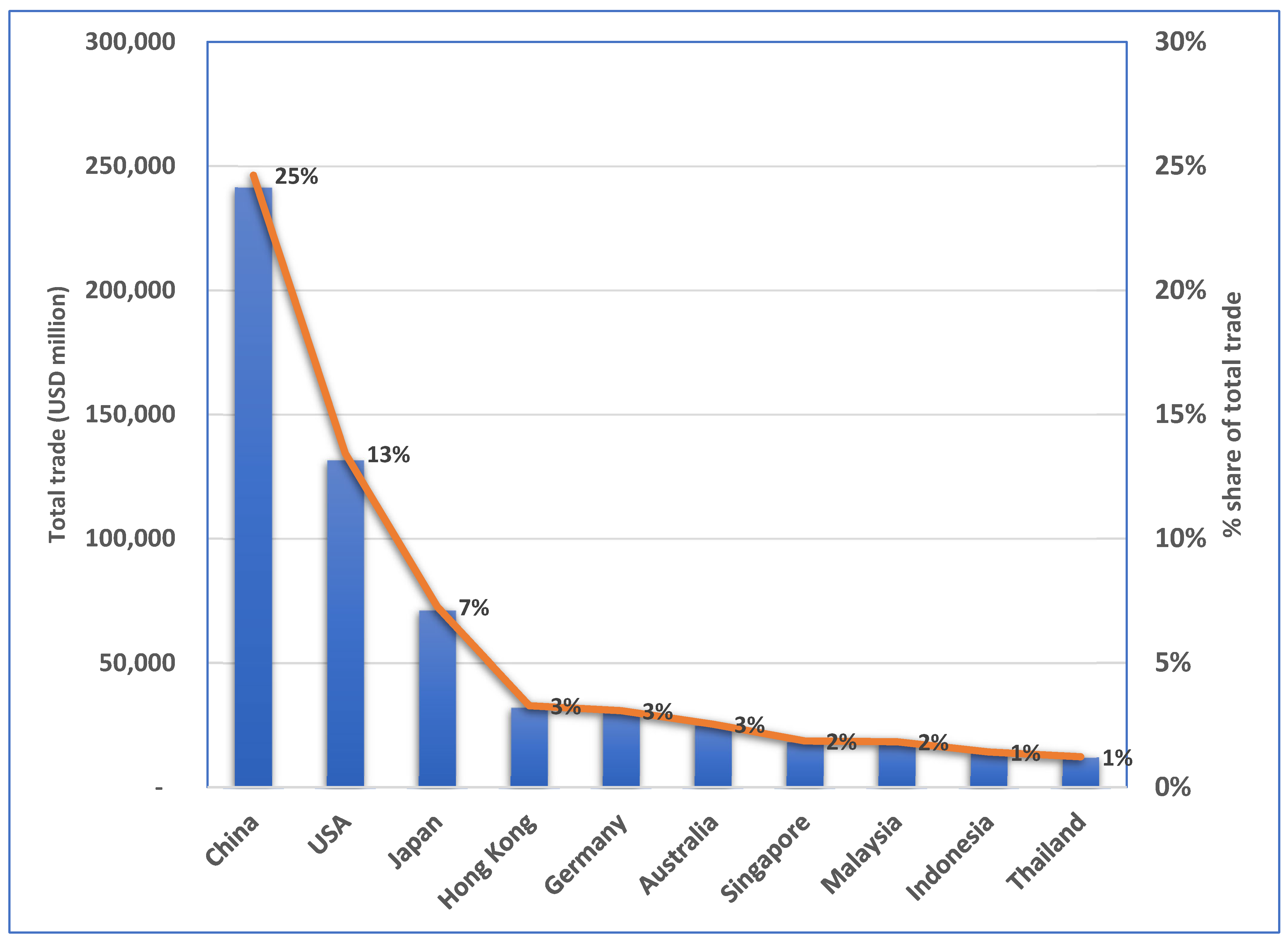
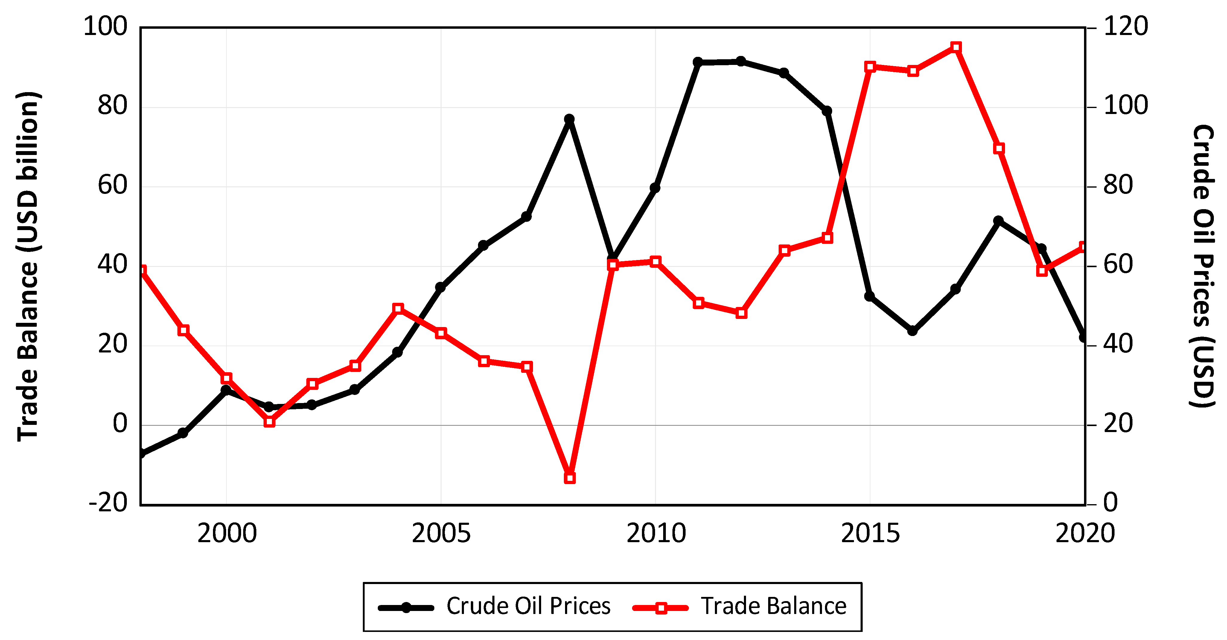
Thus, this article attempts to expand the literature by studying the asymmetric effect that the price of crude oil has on Korea’s exports and imports within the framework of bilateral trade between Korea and its three largest partners, controlling for world trade policy uncertainty. Starting from the early 1960s, Korea has embraced a growth strategy centered around export-oriented industries, with a primary focus on energy-intensive heavy industries. As a result, Korea has emerged as one of the world’s leading exporters, ranking among the top 7 globally, and has achieved a position within the top 10 economies worldwide. As of 2022, Korea’s three largest partners are China, the United States, and Japan, and constitute about 45% of Korea’s overall trade (Figure 1). Additionally, Korea’s reliance on crude oil imports currently reaches more than 50% to meet its energy demand. Thus, it is interesting from a policy and an empirical standpoint to probe to what extent oil price fluctuations have influenced Korea’s trade flows with its three largest partners (Figure 2). To this purpose, Shin et al.’s [1] approach, known as a nonlinear autoregressive distributed lag (NARDL) method, is applied. A notable advantage of employing the NARDL method is its applicability irrespective of whether the series are I(0) or I(1). By doing so, this method essentially eliminates the need for pre-unit root testing. Additionally, the NARDL model can be transformed into an error correction model (ECM) through a simple linear conversion. The ECM captures the short-term dynamics while imposing restrictions on the long-term equilibrium. Consequently, the NARDL model enables simultaneous estimation of both the short-term and long-term parameters in the model. Thus, the NARDL is considered a highly convenient tool for the current topic. In fact, the majority of the related studies have used the NARDL method when tackling the issue. However, Rafiq et al. [2] and Yalta and Yalta [3] have employed dynamic panel and rolling window methods to investigate the topic. The remaining sections provide the literature review, our model, empirical results, discussion, and conclusions with the data described in Appendix A.
2. Literature Review
A large literature has investigated the trade balance impact of oil price shocks. These studies can be divided into two groups. The first group assumes that the impacts of oil price increases and decreases on the trade balance have the same magnitude but in opposite signs, and uses symmetric linear regression (SLR) analysis in examining the subject. See, among others, Svensson [4], Backus and Crucini [5], Kilian et al. [6], Ozlale and Pekkurnza [7], Le and Chang [8], Acikalin and Ugurlu [9], Tiwari et al. [10], Huntington [11], Gnimassoun et al. [12], Olayungbo [13], Musau and Veka [14], and Balli et al. [15]. For instance, Kilian et al. [6] employ a structural VAR method in studying the trade balance effects of oil prices for numerous oil-exporting/importing economies and conclude that the impacts of oil price increases can vary greatly relying on different types of shocks—oil supply, oil demand, and oil-specific demand shocks. Using the frequency domain approach proposed by Breitung and Candelon [16], Tiwari et al. [10] report that oil price shocks serve as a leading indicator of India’s trade balance across short, medium, and long timeframes. Olayungbo [13] also uses the frequency domain causality test and discovers that oil prices do not affect Nigeria’s trade balance significantly. Lately, Balli et al. [15] study the oil price impacts on the trade balance of China and Russia using the time-varying parameter VAR (TVP-VAR) and reveal that oil demand shocks tend to improve (deteriorate) the trade balance of Russia (China).
The second group argues that, since the trade balance responds to oil price increases and decreases differently in practice, the empirical outcomes of the first group relying on SLR analysis could be concerned with possible model misspecification. Thus, this group adopts asymmetric nonlinear regression (NLR) techniques to deal with the subject—see, among others, Allegret et al. [17], Rafiq et al. [2], Raheem [18], Yalta and Yalta [3], Baek et al. [19], Baek and Kwon [20], Ahad and Anwer [21], Baek and Choi [22], and Baek [23]. For instance, Baek and Kwon [20] use a nonlinear ARDL method to test whether oil prices asymmetrically affect the trade balance of six African economies and conclude that there is a significant asymmetric impact on the oil trade balance, but with little evidence on the non-oil and total trade balance. Using the same technique, Ahad and Anwer [21] study the asymmetric effect of oil price shocks on Pakistan’s trade deficit and show that the trade deficit deteriorates as oil prices go up. There are a few studies that have attempted to examine asymmetric effects of exchange rates and/or oil prices and/or economic policy uncertainty on the trade balance or output or renewable energy consumption for Asian economies, including Korea (e.g., Ebrahimi et al. [24]; Khan et al. [25]; Rong et al. [26]). In addition, some studies have examined the asymmetric impacts of oil prices on stock markets (Sadorsky [27,28]; Huang [29]). Using the wavelet transform and VAR methods, for example, Huang [29] concludes that the asymmetric effect of oil prices does not exist for the Shanghai composition index across multiple time scales.
Thus far, a couple of studies have explored the asymmetric relationship between oil prices and Korea’s trade flows (Baek and Choi [22]; Baek [23]). However, their work commonly deals with the trade balance measured in trade surplus in their analysis. Consequently, the misinterpretation of trade balance dynamics in response to oil price shocks can occur. Thus, there exists a significant demand for a well-designed and comprehensive analysis of the interplay between asymmetry in oil prices and the trade balance, which this article endeavors to provide.
3. The Models
In testing the asymmetry impacts that oil prices have on Korea’s trade, the export and import models developed by Baek [30] are modified to empirically encompass oil price fluctuations. In the international trade literature, two key variables that are commonly recognized as significant determinants of a country’s exports (imports) are foreign (domestic) income and exchange rates. These factors have been extensively studied and documented (e.g., Baek [30]). In our empirical model, we go beyond the standard models by incorporating oil prices as an additional determinant, following the approach adopted in other studies (e.g., Baek [23]). By including oil prices in our analysis, we aim to capture the influence of this variable on the dynamics of Korea’s exports and imports, alongside income and exchange rates.
Here, () is the value of Korean exports to (imports from) partner i. If income growth in partner i () and Korea () boosts exports and imports, it is expected that > 0 and > 0. If depreciation of the real Korean exchange rate against partner i () increases (declines) exports (imports) via a fall (rise) in export (import) prices, it is expected that > 0 and 0. The coefficients on are expected to be negative if a rise in oil prices detrimentally influences Korea’s exports and imports via a spike in oil prices and hence costs of production.
Remember that (1) and (2) implicitly assume that oil prices affect Korea’s exports and imports symmetrically. To include asymmetry of oil prices appropriately, in both models is replaced with oil price increases () and oil price decreases (). The partial sum concept is used for this purpose. For instance, , . Then, (1) and (2) become
Now, Equations (3) and (4) should be rewritten as error correction equations, as recommended by Shin et al. [1]:
Once (5) and (6) are estimated by the NARDL, the parameters of α0–α6 and β0–β6t give the short-run impacts. The parameters of − divided by in Equation (5) and of − divided by in Equation (6) denote the long-run impacts. Shin et al. [1] recommend two cointegration tests—that is, F and t-tests—to avoid spurious estimates. In (6), for instance, the F-test decides whether a set of , , , , and is jointly significant. The t-test determines whether is different from zero. Finally, the Wald statistic can be adopted for testing asymmetry. In Equation (5), for instance, the null hypothesis () represents symmetry in the short-run (long-run).
4. Empirical Results
Before discussing the empirical findings, a modeling issue to be addressed is that, since the NARDL can only be applied to series that are either I(1) or I(0), a unit root test should be conducted to ensure that the series are not I(2). However, a conventional unit root test does not consider breaks in the series, which can substantially reduce the power of the test in the presence of a structural break. To overcome this limitation, the test developed by Perron and Vogelsang [31] is used to determine whether the series being tested is not I(2). This test verifies that none of the series in (5) and (6) exceed I(1) processes (Table 1). Thus, the NARDL can be safely applied to the current topic.
Now, let us first discuss the long-run outcomes of the export models (Table 2). It is uncovered that and are statistically significant at the 10% level for the three partners except for the coefficient on in the export model that belongs to China. Thus, oil prices appear to play an important role in fluctuating Korea’s exports to its three largest partners in the long run. To justify the long-run relationship in (5), a convincing case must be made to establish the cointegration of the five series. When using the F- and t-values, cointegration for China and Japan is identified. However, there is little evidence of cointegration for the U.S., so the U.S. is eliminated for further discussion.
The coefficients on are highly significant for China and Japan. The significant coefficients are positive and hint that in the long run, Korea’s exports increase as the Chinese (Japanese) income grows. The coefficient on has a significantly negative impact on China. This suggests that KRW depreciation is likely to decline Korea’s goods exported to China in the long run. The coefficient on is highly significant for China. The significant estimate is negative and suggests that higher trade uncertainty appears to have a depressing effect on Korea’s goods exported to China.
The outcomes of the short-run impacts are now being examined (Table 1). It is revealed that the coefficients on () are highly significant for Japan (China and Japan). In the short run, therefore, it seems that oil prices are important for explaining the variations in Korea’s goods exported to China and Japan. Finally, it is found that the coefficients on , , and are highly significant for China and Japan, indicating that the short-run outcomes give more significant estimates than the long-run results. This finding seems to be counterintuitive as the short-run impacts are more likely to be smaller due to low price elasticities. One possibility is that over time, Korean exporters may have diversified their export markets, thereby reducing their reliance on China and Japan. Diversification helps to spread risk and decrease vulnerability to short-term fluctuations triggered by changes in macroeconomic factors in a specific market. Accordingly, the long-run effects of changes in income, exchange rate, and uncertainty on Korea’s exports to China and Japan may be dampened as a result of increased diversification.
Let us move on to the long-run outcomes from the import models (Table 3). It is observed that the coefficient on () is statistically significant for Japan (China), while neither nor is significant for the U.S. Thus, it turns out that oil prices significantly determine Korea’s imports from China and Japan. Furthermore, the significance of the F- and t-values validate the long-run relationships.
The variable on has a significantly positive (negative) effect on China (the U.S.). This means that Korea’s economic growth would likely push up (down) Korea’s imports from China (the U.S.) via the increase in the domestic purchasing power (domestic production to substitute for imports). The variable has a significantly negative (positive) effect on China (the U.S.), meaning that KRW depreciation drives down (up) Korea’s imports from China (the U.S.) in the long run. The variable is highly significant for China and the U.S. The significant estimate is negative (positive) for China (the U.S.) and suggests that higher trade uncertainty appears to have a detrimental (beneficial) effect on Korea’s goods imported from China (the U.S.).
Next, the focus shifts to the short-run outcomes. When first looking at oil prices, it is discovered that the coefficients on ( and ) are statistically significant for China (Japan), implying significant short-run impacts of oil prices on Korean goods imported from China and Japan. In addition, the short-run coefficients on , , and are significant for all three partners. As with the export models, therefore, these variables are more important in explaining fluctuations of Korea’s imports from its largest three partners in the short run than they do in the long run. Finally, the outcomes from several diagnostic tests disclose that models in (5) and (6) seem well-defined.
To make a comparison, we employ the ARDL method to estimate (5) and (6) (refer to Appendix A, Table A1 and Table A2). An interesting observation emerges; the impacts of oil prices appear to be even more substantial in the NARDL model compared to the ARDL model. Furthermore, when accounting for oil price asymmetry, the F- and t-statistics for cointegration significantly increase. Consequently, these findings provide evidence supporting the notion that incorporating the nonlinearity of oil prices in (5) and (6) is crucial.
5. Discussion
Recall that the primary interest of this article is to identify an indication of whether oil prices asymmetrically influence Korea’s exports and imports. When looking at the export models, it is observed that the coefficients on oil price increases in each of the three models seem to differ from the corresponding coefficients on oil price decreases in terms of magnitudes in the long and short run. Thus, long- and short-run asymmetry appears to exist. To test this hypothesis, however, the Wald statistic should be obtained. In the long run, for example, the statistic based on the distribution is above (below) the 10% critical value for Japan (China). Thus, asymmetric long-run effects are verified only in Japan. This means that Korea’s goods exported to Japan behave differently to oil price increases and decreases. In the short run, however, the hypothesis of symmetry cannot be rejected for both countries. In other words, there is no evidence of short-run asymmetries for Korea’s exports to China and Japan.
When turning to the import models, as with the export models, the fact that the coefficients on oil price increases across models reveal various magnitudes compared to the corresponding coefficients on oil price decreases leads us to suspect that there seems to be asymmetry in the long and short run. Again, the Wald test should be conducted to ensure the reliability of our observation. When the statistics are obtained, the long-run asymmetry effects are affirmative for China and Japan. However, there is no evidence of asymmetric short-run effects for both partners. Thus, this discovery, taken together with the export models, would seem to imply that asymmetry of oil prices is considered a long-run phenomenon. This finding is at odds with Baek and Choi [22] and Baek [23] who discover that oil price changes have asymmetric effects on Korea’s trade balance (measured in trade surplus) in both the long and short run. Another notable finding would be that the asymmetric long-run effect holds for Korea’s exports to and imports from Japan.
The asymmetric effect of oil prices on Korea’s exports to and imports from Japan (China) may be due to the differences in the structure of their economies. If there are limited alternatives or substitutes for the products being traded between Korea and Japan (China), changes in oil prices can have a significant impact on the cost of production and transportation. This can lead to an asymmetrical response, where the effects of oil price increases are more pronounced than the effects of decreases. Alternatively, market demand may play a role in determining the asymmetry effect. For example, if the demand for Korean products in Japan is more price-sensitive than the demand for Japanese products in Korea, changes in production costs resulting from oil price fluctuations may have a greater influence on Korea’s exports to Japan compared to Japan’s exports to Korea.
6. Concluding Remarks
The response of the trade balance to oil price increases and decreases is different in practice. In this short empirical paper, the NARDL is employed to inspect the asymmetric effects that oil prices have on Korean exports to and imports from its three largest partners, controlling for world trade policy uncertainty. The results show evidence validating the long-run asymmetry of oil prices for Korea’s exports to Japan and imports from China and Japan. However, the short-run asymmetry of oil prices does not hold for the three largest partners. Thus, the asymmetries of oil prices are regarded as a long-run phenomenon for Korea’s trade flows with its largest partners. To our knowledge, this is a situation that has not been documented yet in the literature. Other evidence reveals that world trade policy uncertainty plays a more important role in fluctuating Korea’s trade flows with its largest partners in the short run than in the long run.
Our empirical findings have important implications for policymakers, practitioners, and analysts. Firstly, policymakers in the Korean government should consider the asymmetry of oil prices across different trading partners and time horizons (short run vs. long run) when analyzing bilateral trade dynamics. This consideration is crucial to prevent abrupt fluctuations in the trade balance. In instances where an increase in oil prices leads to a total trade deficit due to a decline in exports, the Korean government may need to implement measures to boost exports. These measures could include encouraging banks to increase lending, expanding export credit insurance, and raising tax rebates for relevant firms. Secondly, given the significance of trade uncertainty in Korea’s bilateral trade, particularly in the short run, the Korean government should closely monitor international trade risk situations to maintain export competitiveness in the global market. Additionally, trade practitioners can enhance their risk management strategies to mitigate the impact of trade uncertainty. This may involve financial risk hedging, obtaining trade credit insurance, or exploring alternative financing options. Furthermore, building resilience in the supply chain can help mitigate disruptions caused by trade uncertainty. This includes identifying alternative suppliers, establishing backup production facilities, and maintaining buffer stocks of critical inputs. Thirdly, when examining the impact of oil prices on Korea’s trade with China and Japan, it is crucial to account for the long-run asymmetries of oil prices. Failure to do so could result in misleading outcomes due to model misspecification. Incorporating these long-run asymmetries into empirical models improves the accuracy of analyses and ensures more reliable findings.
It is important to note that this article does not examine the validity of the conjecture that using bilateral exports and imports of commodities reduces the problem of aggregate bias. Furthermore, accurately measuring the effects of oil price changes on Korea’s bilateral trade would require controlling for factors such as oil price volatility and/or technological innovations in the export and import models. Finally, considering that structural breaks in the series can influence the outcomes of oil price asymmetry, it is recommended that future research simultaneously estimate both the asymmetric effects and structural breaks. By considering structural breaks using the Bai and Perron technique, for example, Raheem [18] examines the asymmetric relationship between oil prices and trade components such as exports, imports, and trade openness for high trading, oil importing, and oil exporting economies. Addressing these issues in future studies would contribute to a more comprehensive understanding of the topic. It also should be added that the nonlinear nature of the relationship between crude oil prices and other variables has sparked a growing interest in employing multiscale modeling approaches, such as empirical mode decomposition (EMD) techniques. These methods allow for the identification and analysis of different frequency components within the data, offering a more detailed understanding of the complex interactions between oil prices and other factors. By incorporating EMD techniques into the analysis, researchers can uncover valuable insights into the multiscale dynamics and relationships involved in the study of crude oil prices and related variables.
Funding
This research received no external funding.
Data Availability Statement
The author is willing to share the data in Excel format with those who wish to replicate the results of this study.
Acknowledgments
The author thanks the three referees for their careful reading of my manuscript and their many insightful comments and suggestions that improved the quality of the initial manuscript. Any remaining errors are my sole responsibility. This research is financially supported by the award from the University of Alaska Foundation Harold T. Caven Professorship.
Conflicts of Interest
The author declares no conflict of interest.
Appendix A
Variable Definition and Data Sources (The Author Is Willing to Share the Data in Excel Format with Those Who Wish to Replicate the Results of This Study)
The period of study is 2000:M1 through 2021:M12.
Sources:
- Korea Trade Statistics of the Kora International Trade Association (KITA).
- U.S. Energy Information Administration (EIA).
- The IMF International Financial Statistics (IFS).
- The Economic Policy Uncertainty Group.
- Economic Statistics of the Bank of Korea (ECOS).
Variables:
= value of Korea’s exports to partner i (source a). The nominal value (measured in millions of USD) is deflated by the Korean export price index (2010 = 100) taken from source c.
= value of Korea’s imports from partner i (source a). The nominal value (measured in millions of USD) is deflated by the Korean import price index (2010 = 100) obtained from source c.
= the real exchange rate of Korean won (KRW) per partner i’s currency (source e), indicating KRW appreciates as qt declines. The real exchange rate is defined as CPI* × e/CPI, where CPI* and CPI are consumer price index in partner i and Korea, respectively (source c), and e is the nominal exchange rate (source a).
= the 2010 real income of Korea proxied by industrial production index (source c).
= the 2010 real income of partner i proxied by industrial production index (source c).
= the price of crude oil proxied by the Dubai oil prices (source b). The nominal price (measured in USD) is deflated by the Korean CPI obtained from source c.
= the trade policy uncertainty proxied by the world trade policy uncertainty index (source d).

Table A1.
The oil price impacts on Korea’s exports to its top 3 partners using ARDL.
| China | USA | Japan | |
|---|---|---|---|
| Panel A: long-run outcomes | |||
| 0.06 (1.23) | 0.14 (1.87) * | 0.63 (4.16) ** | |
| −0.10 (2.92) ** | −0.46 (0.63) | −0.42 (0.48) | |
| 0.06 (1.23) | 0.89 (8.31) ** | 0.13 (0.27) | |
| 0.06 (1.23) | 0.03 (0.55) | 0.27 (2.14) ** | |
| Constant | 3.52 (4.54) ** | 0.11 (2.82) ** | 0.46 (3.70) ** |
| Panel B: Short-run outcomes | |||
| 0.08 (1.79) * | 0.03 (2.20) ** | 0.05 (2.77) ** | |
| 0.02 (1.68) * | |||
| 0.08 (1.79) * | 0.03 (2.20) ** | 0.05 (2.77) ** | |
| 0.40 (11.18) ** | −0.02 (0.59) | 0.64 (8.07) ** | |
| −0.07 (1.09) | 0.54 (5.76) ** | ||
| −0.09 (1.39) | 0.66 (6.02) ** | ||
| −0.13 (2.59) ** | 0.34 (3.58) ** | ||
| 0.06 (1.66) | 0.29 (3.35) ** | ||
| −1.40 (5.16) ** | 0.96 (82.95) ** | −0.26 (1.63) | |
| 0.51 (1.77) * | −0.34 (5.66) ** | ||
| 0.14 (2.36) ** | |||
| −0.03 (1.87) * | 0.001 (0.56) | 0.02 (2.44) ** | |
| 0.01 (0.43) | |||
| 0.05 (3.41) ** | |||
| Panel C: diagnostic statistics | |||
| F-statistic | 3.98 * | 1.57 | 2.64 |
| t-statistic | −0.30 (4.54) ** | −0.05 (2.82) | −0.09 (3.65) |
| LM | 0.39 | 0.05 | 3.27 |
| RESET | 1.01 | 1.95 | 9.01 |
| CU (CUS) | S (S) | S (S) | S (S) |
** and * denote the 5 percent and 10 percent significance levels, respectively. The numbers in parentheses are the absolute t-statistics. The 5 percent and 10 percent critical values for the F-test (t-test) are 4.01 (−3.99) and 3.52 (−3.66), respectively. LM and RESET represent chi-squared statistics to test for no residual serial correlation and no functional misspecification, respectively.
Table A2.
The oil price impacts on Korea’s imports from its top 3 partners using ARDL.
| China | USA | Japan | |
|---|---|---|---|
| Panel A: long-run outcomes | |||
| −0.47 (4.84) ** | −0.01 (0.19) | −1.27 (0.86) | |
| 3.01 (15.76) ** | −0.62 (3.52) ** | 1.28 (0.81) | |
| −2.12 (7.44) ** | 0.89 (8.10) ** | −0.29 (0.36) | |
| −0.11 (1.81) * | 0.15 (4.02) ** | −0.63 (0.94) | |
| Constant | 1.29 (6.28) ** | 0.89 (7.12) ** | 0.42 (3.99) ** |
| Panel B: Short-run outcomes | |||
| −0.15 (3.25) ** | −0.003 (0.19) | −0.13 (2.62) ** | |
| −0.22 (4.48) ** | −0.10 (1.99) ** | ||
| 0.16 (3.26) ** | |||
| 1.21 (17.00) ** | 0.58 (5.76) ** | 0.96 (10.86) ** | |
| 0.68 (7.17) ** | 0.49 (4.34) ** | 0.32 (2.68) ** | |
| 0.45 (4.14) ** | −0.15 (1.46) | ||
| 0.49 (4.49) ** | 0.37 (3.51) ** | ||
| 0.39 (3.85) ** | 0.48 (4.43) ** | ||
| 0.33 (3.74) ** | 0.20 (2.44) ** | ||
| −0.84 (4.45) ** | 0.27 (5.65) ** | −0.50 (3.35) ** | |
| −0.67 (3.15) ** | |||
| −0.02 (1.91) * | −0.001 (0.06) | −0.02 (2.46) ** | |
| −0.05 (2.29) ** | |||
| −0.03 (1.36) | |||
| −0.06 (2.80) ** | |||
| −0.03 (1.44) | |||
| Panel C: diagnostic statistics | |||
| F-statistic | 7.61 ** | 10.13 ** | 3.23 |
| t-statistic | −0.15 (6.22) ** | −0.30 (7.18) ** | −0.04 (4.05) ** |
| LM | 1.17 | 1.28 | 3.40 * |
| RESET | 4.84 ** | 0.21 | 0.31 |
| CU (CUS) | S (S) | S (S) | S (S) |
** and * denote the 5 percent and 10 percent significance levels, respectively. The numbers in parentheses are the absolute t-statistics. The 5 percent and 10 percent critical values for the F-test (t-test) are 4.01 (−3.99) and 3.52 (−3.66), respectively. LM and RESET represent chi-squared statistics to test for no residual serial correlation and no functional misspecification, respectively.
References
- Shin, Y.; Yu, B.; Greenwood-Nimmo, M. Modelling Asymmetric Cointegration and Dynamic Multipliers in a Nonlinear ARDL Framework. In Festschrift in Honor of Peter Schmidt: Econometric Methods and Applications; Sickels, R., Horrace, W., Eds.; Springer: Berlin/Heidelberg, Germany, 2014; pp. 281–314. [Google Scholar]
- Rafiq, S.; Sgro, P.; Apergis, N. Asymmetric oil shocks and external balances of major oil exporting and importing countries. Energy Econ. 2016, 56, 42–50. [Google Scholar] [CrossRef]
- Yalta, A.Y.; Yalta, A.T. Dependency on imported oil and its effects on current account. Energy Sources Part B Econ. Plan. Policy 2017, 12, 859–886. [Google Scholar] [CrossRef]
- Svensson, L.E. Oil Prices, Welfare, and the Trade Balance. Q. J. Econ. 1984, 99, 649–672. [Google Scholar] [CrossRef]
- Backus, D.K.; Crucinic, M.J. Oil Prices and the Terms of Trade. J. Int. Econ. 2000, 50, 185–213. [Google Scholar] [CrossRef] [Green Version]
- Killian, L.; Rubucci, A.; Spatafora, N. Oil Shocks and External Balances. J. Int. Econ. 2009, 77, 181–194. [Google Scholar] [CrossRef] [Green Version]
- Özlale, U.; Pekkurnaz, D. Oil prices and current account: A structural analysis for the Turkish economy. Energy Policy 2010, 38, 4489–4496. [Google Scholar] [CrossRef]
- Le, T.-H.; Chang, Y. Oil price shocks and trade imbalances. Energy Econ. 2013, 36, 78–96. [Google Scholar] [CrossRef]
- Acikalin, S.; Ugurlu, E. Oil Price Fluctuations and Trade Balance of Turkey. Procedia Econ. Bus. Adm. 2014, 1, 6–13. [Google Scholar]
- Tiwari, A.K.; Arouri, M.; Teulon, F. Oil Prices and Trade Balance: A Frequency Domain Analysis for India. Econ. Bull. 2014, 34, 663–680. [Google Scholar]
- Huntington, H.G. Crude oil trade and current account deficits. Energy Econ. 2015, 50, 70–79. [Google Scholar] [CrossRef]
- Gnimassoun, B.; Joets, M.; Razafindrabe, T. On the Link between Current Account and Oil Price Fluctuations in Diversified Economies: The Case of Canada. Int. Econ. 2017, 152, 63–78. [Google Scholar] [CrossRef] [Green Version]
- Olayungbo, D.O. Effects of Global Oil Price on Exchange Rate, Trade Balance, and Reserves in Nigeria: A Frequency Domain Causality Approach. J. Risk Financ. Manag. 2019, 12, 43. [Google Scholar] [CrossRef] [Green Version]
- Musau, A.; Veka, S. Crude oil trade and current account deficits: Replication and extension. Empir. Econ. 2020, 58, 875–897. [Google Scholar] [CrossRef]
- Balli, E.; Çatık, A.N.; Nugent, J.B. Time-varying impact of oil shocks on trade balances: Evidence using the TVP-VAR model. Energy 2021, 517, 119377. [Google Scholar] [CrossRef]
- Breitung, J.; Candelon, B. Testing for short- and long-run causality: A frequency-domain approach. J. Econom. 2006, 132, 363–378. [Google Scholar] [CrossRef]
- Allegret, J.-P.; Couharde, C.; Coulibaly, D.; Mignon, V. Current accounts and oil price fluctuations in oil-exporting countries: The role of financial development. J. Int. Money Financ. 2014, 47, 185–201. [Google Scholar] [CrossRef] [Green Version]
- Raheem, I.D. Asymmetry and break effects of oil price -macroeconomic fundamentals dynamics: The trade effect channel. J. Econ. Asymmetries 2017, 16, 12–25. [Google Scholar] [CrossRef]
- Baek, J.; Ikponmwosa, M.J.; Choi, Y.J. Crude oil prices and the balance of trade: Asymmetric evidence from selected OPEC member countries. J. Int. Trade Econ. Dev. 2019, 28, 533–547. [Google Scholar] [CrossRef]
- Baek, J.; Kwon, K.D. Asymmetric effects of oil price changes on the balance of trade: Evidence from selected African countries. World Econ. 2019, 42, 3235–3252. [Google Scholar] [CrossRef]
- Ahad, M.; Answer, Z. Asymmetrical Relationship between Oil Price Shocks and Trade Deficit: Evidence from Pakistan. J. Int. Trade Econ. Dev. 2020, 29, 163–180. [Google Scholar] [CrossRef]
- Baek, J.; Choi, Y.J. Do oil price changes really matter to the trade balance? Evidence from Korea-ASEAN commodity trade data. Aust. Econ. Pap. 2020, 59, 250–278. [Google Scholar]
- Baek, J. An asymmetric approach to the oil prices-trade balance nexus: New evidence from bilateral trade between Korea and her 14 trading partners. Econ. Anal. Policy 2020, 68, 199–209. [Google Scholar] [CrossRef]
- Ebrhimi, M.; Kiani, K.H.; Memarnejad, A.; Ghaffari, F. Nonlinear Asymmetric Effects of Devaluation on Trade Balance: A Case Study of Iran and South Korea. J. Money Econ. 2018, 13, 51–61. [Google Scholar]
- Khan, M.A.; Husnain, M.I.U.; Abbas, Q.; Shah, S.Z.A. Asymmetric Effects of Oil Price Shocks on Asian Economies: A Nonlinear Analysis. Empir. Econ. 2019, 57, 1319–1350. [Google Scholar] [CrossRef]
- Rong, G.; Qamruzzzman, M. Symmetric and Asymmetric Nexus between Economic Policy Uncertainty, Oil Prices, and Renewable Energy Consumption in the United States, China, India, Japan, and South Korea: Does Technological Innovation Influence? Front. Energy Res. 2022, 10, 973557. [Google Scholar] [CrossRef]
- Sadorsky, P. The macroeconomic determinants of technology stock price volatility. Rev. Financ. Econ. 2003, 12, 191–205. [Google Scholar] [CrossRef]
- Sadorsky, P. Correlations and volatility spillovers between oil prices and the stock prices of clean energy and technology companies. Energy Econ. 2012, 34, 248–255. [Google Scholar] [CrossRef]
- Huang, S.; Haizhong, A.; Gao, X.; Sun, X. Do Oil Price Symmetric Effects on the Stock Market Persistent in Multiple Time Horizons? Appl. Energy 2017, 185, 1799. [Google Scholar] [CrossRef]
- Baek, J. Exchange Rate Sensitivity of Korea-U.S. Bilateral Trade: Evidence from Industrial Trade Data. J. Korea Trade 2012, 16, 1–21. [Google Scholar]
- Perron, P.; Vogelsang, T.J. Testing for a Unit Root in a Time Series with a Changing Mean: Corrections and Extensions. J. Bus. Econ. Stat. 1992, 10, 467–470. [Google Scholar]
Figure 1.
Korea’s top 10 trading partners (2020) for no residual serial correlation and no functional misspecification, respectively.
Figure 1.
Korea’s top 10 trading partners (2020) for no residual serial correlation and no functional misspecification, respectively.

Figure 2.
Korea’s trade balance and crude oil prices.

Table 1.
Results of Perron–Vogelsang unit root tests.
| Level | Time Break | First Difference | Time Break | Decision | ||
|---|---|---|---|---|---|---|
| y | China | −10.81 (12) ** | 2011M02 | I(0) | ||
| U.S. | −4.50 (14) | 2008M7 | −20.85 (0) ** | 2000M6 | I(1) | |
| Japan | −9.01 (0) ** | 2001M5 | I(0) | |||
| Korea | −6.01 (0) ** | 2001M1 | I(0) | |||
| q | China | −3.72 (2) | 2007M10 | −12.72 (1) ** | 2008M10 | I(1) |
| U.S. | −7.18 (0) ** | 2000M12 | I(0) | |||
| Japan | −3.77 (1) | 2008M8 | −14.89 (0) ** | 2008M10 | I(1) | |
| e | China | −4.42 (0) | 2002M2 | −19.57 (0) ** | 2001M1 | I(1) |
| U.S. | −8.63 (0) ** | 2000M12 | I(0) | |||
| Japan | −3.95 (0) | 2001M4 | −23.01 (0) ** | 2001M1 | I(1) | |
| m | China | −5.40 (0) ** | 2001M2 | I(0) | ||
| U.S. | −5.89 (1) ** | 2008M1 | I(0) | |||
| Japan | −5.85 (0) ** | 2001M5 | I(0) | |||
| Oil Price+ | −4.09 (1) | 2012M8 | −13.91 (0) ** | 2009M6 | I(1) | |
| Oil Price− | −3.91 (1) | 2014M9 | −11.64 (0) ** | 2020M3 | I(1) |
Notes: ** indicate rejection of the null hypothesis at the 5% level. The 5% and 10% critical values for the DF-GLS (Perron-Vogelsang), including a constant and trend, are −2.990 (−5.175) and −2.700 (−4.893), respectively. Parentheses are lag lengths.
Table 2.
The oil price impacts on Korea’s exports to its top 3 partners.
| China | USA | Japan | |
|---|---|---|---|
| Panel A: long-run outcomes | |||
| 0.04 (0.81) | 0.13 (2.15) ** | 0.40 (4.88) ** | |
| 0.08 (1.71) * | 0.17 (1.94) * | 0.30 (3.08) ** | |
| 0.98 (6.39) ** | −1.49 (1.51) | 1.35 (1.96) ** | |
| −1.04 (2.61) ** | 1.19 (3.81) ** | 0.33 (1.22) | |
| −0.08 (2.67) ** | 0.03 (0.61) | −0.004 (0.06) | |
| Constant | 4.04 (5.79) ** | 0.35 (3.40) ** | −0.22 (4.10) ** |
| Panel B: Short-run outcomes | |||
| 0.01 (0.11) | 0.10 (3.67) ** | 0.07 (3.30) ** | |
| −0.16 (1.42) | 0.04 (1.37) | ||
| 0.16 (1.54) | −0.03 (1.04) | ||
| −0.002 (0.02) | −0.01 (0.39) | 0.05 (2.64) ** | |
| 0.25 (2.57) ** | 0.02 (0.87) | ||
| −0.31 (3.39) ** | 0.06 (2.41) ** | ||
| 0.41 (11.97) ** | −0.10 (1.60) | 0.68 (8.83) ** | |
| −0.16 (3.26) ** | 0.37 (3.70) ** | ||
| −0.16 (3.40) ** | 0.55 (4.93) ** | ||
| −0.12 (2.83) ** | 0.26 (2.77) ** | ||
| 0.05 (1.40) | 0.26 (3.04) ** | ||
| −1.24 (4.72) ** | 0.96 (78.26) ** | −0.35 (2.16) ** | |
| 0.54 (2.02) ** | −0.35 (5.56) ** | ||
| 0.13 (1.89) * | |||
| −0.09 (1.32) | |||
| 0.03 (0.41) | |||
| −0.16 (2.78) ** | |||
| −0.02 (1.76) * | 0.01 (2.09) ** | −0.35 (2.16) ** | |
| 0.01 (0.55) | |||
| 0.06 (4.07) ** | |||
| Panel C: diagnostic statistics | |||
| F-statistic | 5.36 ** | 1.92 | 2.90 |
| t-statistic | −0.39 (5.79) ** | −0.07 (3.43) ** | −0.17 (4.22) ** |
| LM | 2.38 | 3.61 | 0.98 |
| RESET | 0.29 | 1.70 | 0.06 |
| CU (CUS) | S (S) | S (S) | S (S) |
** and * denote the 5 percent and 10 percent significance levels, respectively. The numbers in parentheses are the absolute t-statistics. The 5 percent and 10 percent critical values for the F-test (t-test) are 3.79 (−4.19) and 3.35 (−3.86), respectively. LM and RESET represent chi-squared statistics to test for no residual serial correlation and no functional misspecification, respectively.
Table 3.
The oil price impacts on Korea’s imports from its top 3 partners.
| China | USA | Japan | |
|---|---|---|---|
| Panel A: long-run outcomes | |||
| −0.18 (1.53) | −0.01 (0.14) | −2.53 (1.90) * | |
| −0.28 (3.13) ** | −0.01 (0.22) | 2.02 (0.87) | |
| 1.99 (4.86) ** | −0.64 (1.81) * | 6.26 (0.96) | |
| −2.08 (9.40) ** | 0.90 (7.89) ** | 0.49 (0.36) | |
| −0.12 (2.32) ** | 0.14 (3.22) ** | −0.30 (0.63) | |
| Constant | 2.05 (6.91) ** | 0.86 (6.98) ** | −0.66 (4.58) ** |
| Panel B: Short-run outcomes | |||
| −0.14 (1.42) | −0.003 (0.14) | −0.14 (1.34) | |
| −0.06 (0.64) | −0.17 (1.57) | ||
| 0.20 (1.90) * | |||
| −0.14 (1.95) * | −0.004 (0.22) | −0.10 (1.31) | |
| −0.35 (4.73) ** | −0.03 (0.28) | ||
| 0.16 (1.88) * | |||
| 1.18 (16.86) ** | 0.58 (5.82) ** | 0.93 (10.59) ** | |
| 0.71 (7.78) ** | 0.49 (4.40) ** | 0.15 (1.36) | |
| 0.45 (4.16) ** | −0.36 (3.65) ** | ||
| 0.48 (4.43) ** | 0.22 (2.09) ** | ||
| 0.37 (3.67) ** | 0.27 (2.82) ** | ||
| 0.33 (3.69) ** | |||
| −0.92 (4.91) ** | 0.26 (5.54) ** | −0.39 (2.56) ** | |
| −0.63 (2.99) ** | −0.21 (1.34) | ||
| 0.14 (0.89) | |||
| −0.24 (1.53) | |||
| −0.25 (1.66) * | |||
| −0.23 (1.57) | |||
| −0.02 (2.41) ** | −0.001 (0.07) | −0.03 (1.90) * | |
| −0.04 (2.06) ** | −0.03 (1.95) * | ||
| −0.02 (0.99) | |||
| −0.04 (2.37) | |||
| Panel C: diagnostic statistics | |||
| F-statistic | 7.71 ** | 8.09 ** | 3.33 |
| t-statistic | −0.20 (6.87) ** | −0.29 (7.04) ** | −0.04 (4.52) ** |
| LM | 1.33 | 2.08 | 0.02 |
| RESET | 1.76 | 2.20 | 2.16 |
| CU (CUS) | S (S) | S (S) | S (S) |
** and * denote the 5 percent and 10 percent significance levels, respectively. The numbers in parentheses are the absolute t-statistics. The 5 percent and 10 percent critical values for the F-test (t-test) are 3.79 (−4.19) and 3.35 (−3.86), respectively. LM and RESET represent chi-squared statistics to test.
Disclaimer/Publisher’s Note: The statements, opinions and data contained in all publications are solely those of the individual author(s) and contributor(s) and not of MDPI and/or the editor(s). MDPI and/or the editor(s) disclaim responsibility for any injury to people or property resulting from any ideas, methods, instructions or products referred to in the content. |
© 2023 by the author. Licensee MDPI, Basel, Switzerland. This article is an open access article distributed under the terms and conditions of the Creative Commons Attribution (CC BY) license (https://creativecommons.org/licenses/by/4.0/).
Share and Cite
MDPI and ACS Style
Baek, J. Oil Prices, World Trade Policy Uncertainty, and the Trade Balance: The Case of Korea. Commodities 2023, 2, 188-200. https://doi.org/10.3390/commodities2030012
AMA Style
Baek J. Oil Prices, World Trade Policy Uncertainty, and the Trade Balance: The Case of Korea. Commodities. 2023; 2(3):188-200. https://doi.org/10.3390/commodities2030012
Chicago/Turabian StyleBaek, Jungho. 2023. "Oil Prices, World Trade Policy Uncertainty, and the Trade Balance: The Case of Korea" Commodities 2, no. 3: 188-200. https://doi.org/10.3390/commodities2030012