Evaluation of Vertical Profiles and Atmospheric Boundary Layer Structure Using the Regional Climate Model CCLM during MOSAiC

Abstract

Regional climate models are a valuable tool for the study of the climate processes and climate change in polar regions, but the performance of the models has to be evaluated using experimental data. The regional climate model CCLM was used for simulations for the MOSAiC period with a horizontal resolution of 14 km (whole Arctic). CCLM was used in a forecast mode (nested in ERA5) and used a thermodynamic sea ice model. Sea ice concentration was taken from AMSR2 data (C15 run) and from a high-resolution data set (1 km) derived from MODIS data (C15MOD0 run). The model was evaluated using radiosonde data and data of different profiling systems with a focus on the winter period (November–April). The comparison with radiosonde data showed very good agreement for temperature, humidity, and wind. A cold bias was present in the ABL for November and December, which was smaller for the C15MOD0 run. In contrast, there was a warm bias for lower levels in March and April, which was smaller for the C15 run. The effects of different sea ice parameterizations were limited to heights below 300 m. High-resolution lidar and radar wind profiles as well as temperature and integrated water vapor (IWV) data from microwave radiometers were used for the comparison with CCLM for case studies, which included low-level jets. LIDAR wind profiles have many gaps, but represent a valuable data set for model evaluation. Comparisons with IWV and temperature data of microwave radiometers show very good agreement.

1. Introduction

The impact of the recent global climate change is most pronounced in the Arctic, where the near-surface warming effects are 2–4 times the global average [1,2,3]. This effect, called “Arctic Amplification”, is strongly related to atmosphere–ocean–sea ice (AOI) interactions and their feedbacks between the free atmosphere, the atmospheric boundary layer (ABL), and the surface. On a regional scale, the sea ice changes have led to much larger temperature trends than in the Arctic average [4]. In order to understand the New Arctic and its future development, AOI interactions represent key processes. Regional climate models (RCMs) are an important tool to investigate the processes that are relevant to understanding the New Arctic. In order to include the effects of topographic winds and polynyas, as well as extreme winds, in atmospheric models, a horizontal resolution of 15 km or less is needed [5,6]. Parameterization of the stable boundary layer (SBL) and subgrid processes, such as leads, are major challenges for atmospheric models.

In order to use RCMs for climate and process studies, the performance of the models has to be evaluated using experimental data. However, experiments with measurements of the ABL over Arctic oceans and sea ice are rare, particularly during winter for the inner Arctic, since icebreakers and complex logistics are needed. Recent RCM evaluation studies of the ABL in the Arctic were performed for the Arctic in the summer of 2014 [7,8]. Both studies compared RCM data with radiosonde profiles. Biases varied between −2.0 and +0.8 °C for the temperature in the lowest 1500 m, and the moisture bias was between −0.3 and +0.2 g/kg for the different models. The performance of the operational European Centre for Medium-Range Weather Forecasts (ECMWF) numerical weather prediction model was investigated for summer 2018 in the central Arctic in comparison with radiosondes [9]. They found a warm bias of 0.5–1.0 °C in the lowest 100 m and a large cold bias of 1–2 °C around 1 km. A study during wintertime conditions using radiosondes, a microwave temperature profiler, and microwave-integrated water vapor (IWV) measurements for a four-week drift of an icebreaker in the inner Arctic in April 2019 is described in [10]. This study showed that the representations of the wind, temperature, and moisture structure by the simulations were very good for the ABL and the troposphere. A comparison of wind profiles from SODAR measurements and RCM simulations for a three-year period in the area of Severnaya Zemlya (Siberia) showed a positive bias for a wind speed of about 1 m/s below 100 m, which increased to 1.5 m/s for higher levels [11].

In the present paper, we use ABL measurements from the MOSAiC experiment [12], where multiple instruments measured atmospheric quantities in the ABL for a full year. In contrast to previous experiments of the last 20 years, which were performed over the course of only a few weeks and rarely during winter, MOSAiC covers a complete yearly cycle in the inner Arctic with an unprecedented set of measurement systems for the atmosphere, sea ice, and ocean. The focus of our study is on the winter period (November 2019 to April 2020), when the German research vessel Polarstern drifted with the ice in the inner Arctic, but results for the summer period are also shown. The last experiment comparable to MOSAiC was the SHEBA campaign of 1997–1998 [13], which was also intensively used for model verification and the development of parameterizations [14,15,16]. The aim of the present study is to evaluate the regional climate model CCLM with respect to its performance in simulating atmospheric quantities in the troposphere and the ABL using MOSAiC data.

2. Materials and Methods

2.1. Observations

The German research icebreaker Polarstern was the basis of the MOSAiC experiment. From October 2019 to mid-May 2020, Polarstern drifted from the northern Laptev Sea almost to Svalbard (Figure 1). After an interruption due to logistic reasons (with a stay near Longyearbyen, Svalbard, from 4 to 8 June 2020), a second drift phase took place from the middle of June to the end of July between Svalbard and Greenland. Then, the ship moved close to the north pole, and a third drift phase took place from the end of August to the end of September 2020. A full description of the instrumentation is given in [12]. In the present paper, we used data from the instruments listed in Table 1 for the evaluation of the simulations (see Section 2.2).

All measurements listed in Table 1 were made onboard Polarstern during the experiment. The main data for the evaluation were obtained from radiosondes, which were launched from the helicopter deck of Polarstern every six hours operationally and every three hours during special observation periods (Table 1). We used level-3 soundings, which have been post-processed according to the Global Climate Observing System (GCOS) Reference Upper-Air Network (GRUAN) algorithm, and have a vertical resolution of 5 m [17]. Since the height information was obtained from Global Navigation Satellite Systems (GNSS) data, we followed the recommendations of [17] and recalculated the heights hydrostatically using the observed sensor pressure and the mean sea level pressure measured by the Polarstern’s meteorological system [18]. In order to reduce the volume of the data set and adapt it to the vertical resolution of the simulations, the data were interpolated to vertical grids of 20 m (0–400 m), 40 m (400–1200 m), 60 m (1200–2400 m), 100 m (2400–4400 m), and 200 m (>4400 m), respectively. Only ascents higher than 2000 m were considered. The uncertainties of the radiosonde measurements provided by the manufacturer were 0.3 K for temperature below 16 km height, 4% for relative humidity, and 0.15 m/s and 2° for wind speed and direction, respectively [19]. The GRUAN postprocessing yielded uncertainties for each data point individually, which were larger than the manufacturer values, particularly for wind speed. For the mid-latitudes and the tropics [20], uncertainties of 0.4–1.0 m/s were found for the wind speed. In the MOSAiC data set, the typical uncertainties below 10 km height were 0.2–0.3 K for temperature; 0.02 g/kg and 0.10 g/kg for specific humidity in winter and summer, respectively; and 4 m/s for wind speed (note that the GRUAN uncertainties correspond to two times the standard deviation).

Wind data from the Galion wind lidar [21] were averaged to 1 h means for the comparison with the simulations, using the median of at least three values per hour. The lidar data included an uncertainty estimate [22], and only data with a wind speed error less than 2 m/s were used. Since there were many cases with unrealistic values for the lowest level at 64 m, this level was not considered for the comparison. Radar wind profiler data [23] were used only for the high-resolution mode (for the lower 2000 m). Only data with good-quality flags were used. The temperature profiles of the HATPRO (Humidity and Temperature Profiler) radiometer were retrieved on a height grid with 50 m vertical spacing below 250 m and 75–500 m above 250 m [24]. The true vertical resolution was much coarser, with up to four distinctly resolved height layers allowing us to capture the major temperature profile structure while smoothing out vertical gradients. In the boundary layer mode, the radiometer had an improved vertical resolution in the lowest 2 km compared to the standard zenith-pointing operation. Therefore, we used only averages for the lowest 2 km and data with good-quality flags. IWV data were available from the two microwave radiometers HATPRO and MiRAC-P (Microwave Radiometer for Arctic Clouds—Passive). IWV from the radiometers is reliable in any weather conditions except for strong liquid precipitation or conditions in which snow accumulation on the instruments is a risk. For both data sets, only data with good-quality flags were averaged to 1 h means for the comparison with the simulations.

In addition, we used near-surface data of wind measurements of the Polarstern meteorological system [18] and of a meteorological tower near Polarstern (Met City, [25]). A detailed description of these data is given in [26].

Table 1. Measurements used for the present study.

Quantity	Instrument	Height	Sampling	Data Resolution	Data Provider	Reference
Temperature, Humidity, Wind Speed, and Direction	Radiosonde Vaisala RS41-SGP	10 m–32 km	1 s	3 to 6 h, 5 m vertically	AWI	[17]
Wind Speed and Direction	Galion wind lidar	64–2300 m	5 min	5 min, 23 m vertically	University of Leeds	[21]
	Radar wind profiler	200–2000 m	1 h	1 h, 20 m vertically	Atmospheric Radiation Measurement (ARM) user facility	[23]
Temperature	HATPRO microwave radiometer in boundary layer mode	15 m–10 km	110 s every 30 min	30 min, vertically variable (50–500 m)	University of Cologne, Leibniz Institute of Tropospheric Research	[27]
Integrated Water Vapor	HATPRO microwave radiometer		1 s	1 s	University of Cologne, Leibniz Institute of Tropospheric Research	[27]
	MiRAC-P microwave radiometer		1 s	1 s	University of Cologne	[28]

Table 1. Measurements used for the present study.

Quantity	Instrument	Height	Sampling	Data Resolution	Data Provider	Reference
Temperature, Humidity, Wind Speed, and Direction	Radiosonde Vaisala RS41-SGP	10 m–32 km	1 s	3 to 6 h, 5 m vertically	AWI	[17]
Wind Speed and Direction	Galion wind lidar	64–2300 m	5 min	5 min, 23 m vertically	University of Leeds	[21]
	Radar wind profiler	200–2000 m	1 h	1 h, 20 m vertically	Atmospheric Radiation Measurement (ARM) user facility	[23]
Temperature	HATPRO microwave radiometer in boundary layer mode	15 m–10 km	110 s every 30 min	30 min, vertically variable (50–500 m)	University of Cologne, Leibniz Institute of Tropospheric Research	[27]
Integrated Water Vapor	HATPRO microwave radiometer		1 s	1 s	University of Cologne, Leibniz Institute of Tropospheric Research	[27]
	MiRAC-P microwave radiometer		1 s	1 s	University of Cologne	[28]

2.2. Model Data

The model utilized was the non-hydrostatic regional climate model Consortium for small scales—Climate Limited-Area Mode (CCLM). The setup of CCLM for MOSAiC is described in [26], where CCLM was evaluated using near-surface measurements of MOSAiC. CCLM is run with 14 km horizontal resolution and covers the whole Arctic (Figure 1a). In the vertical direction, the model extends up to 22 km with 60 vertical levels, and 13 levels are below 500 m in order to obtain a high resolution for the boundary layer. The first model level is at 5 m above the surface (

Table 2. Configuration of the CCLM simulations.

Forcing	Vertical/Horizontal Resolutions, Lowest 15 Levels	Run Mode	Sea Ice Concentration (SIC) and Thickness
ERA5 data for lateral boundary fields	60 levels, 14 km 5, 16, 31, 48, 70, 96, 127, 164, 206, 254, 310, 372, 443, 522, 609 m	Forecast mode (reinitialized at 18 UTC, 6-h spin-up), hourly data output	AMSR2 and MODIS (SIC), daily data PIOMAS ice thickness, daily data

), and the time resolution of the model output is 1 h.

Initial data and boundary data with hourly resolution for the simulations were taken from ERA5 data [29]. The simulations were restarted daily, and no nudging was performed during the simulation time of 30 h. This kind of forecast mode was used in several previous evaluation studies [7,8,10,30,31]. Although ERA5 data were used at the boundaries, the CCLM domain was large enough to allow for developments of synoptic and mesoscale systems which were different to ERA5. In addition, the parameterizations of CCLM differed from ERA5, particularly for the ABL and sea ice.

Sea ice concentration (SIC), as shown in Figure 1, was taken as daily data from Advanced Microwave Scanning Radiometer 2 (AMSR2) data with 6 km resolution [32]. In addition, daily SIC and information about sea ice leads were taken from Moderate Resolution Imaging Spectroradiometer (MODIS) data for the period from November 2019 to April 2020 [26]. In [26], different methods to use the MODIS sea ice data were investigated. In the present study, we used the daily SIC from a merged MODIS/AMSR2 product, which was modified by a MODIS lead fraction, where leads were considered to be ice-free in the initial field for CCLM. Sea ice thickness was prescribed daily from the interpolated Pan-Arctic Ice Ocean Modeling and Assimilation System (PIOMAS) fields [33]. For both cases (SIC from AMSR2 or MODIS), the ice-free fraction (1-SIC) was considered in the sub-grid sea ice parameterization in CCLM. The PIOMAS ice thickness was taken for the grid-scale SIC fraction, and the sub-grid thin ice thickness was computed for each model grid point by thermodynamic growth during the daily initialization of the sea ice model (see [10,26]). The runs with AMSR2 data and MODIS data were referred to as C15 and C15MOD0, respectively. SIC from MODIS data was only available for the winter period (November to April). As a consequence, the C15MOD0 run covered only the winter period, while the C15 run covered the whole MOSAiC period from October 2019 to September 2020. For the comparison with the measurements from Polarstern, the closest model grid point was selected for each hour.

3. Results

3.1. Evaluation Using Radiosonde Data

3.1.1. Case Studies

An example of measured and simulated profiles is shown in Figure 2 for a radiosonde launched at 0500 UTC on 1 March 2020, as well as the corresponding simulation for the lowest 10 km. The measured temperature profile showed an inversion in the lowest 1000 m, which was associated with a decrease in wind speed and a shift of the wind direction above the inversion. The simulated profiles agreed very well with the measurements. There was a small underestimation of the specific humidity in the inversion layer, but even the humidity increase at 2000 m was represented well in the simulation. For the wind profile, there were fluctuations in the radiosonde data, which were due to the local nature of the measurements or other problems. Note that the amplitude of the wind fluctuations was within the uncertainty specified by the GRUAN algorithm. Since the simulation captured the mean wind structure well, these fluctuations contributed to the standard deviation (STDV) when comparing the simulations with radiosonde data.

As an example of the comparison for a complete month, Figure 3 shows the time–height cross-sections for temperature and specific humidity for November 2019 and for the lowest 6 km. This month was selected since there were two events with strong moisture intrusions on 16 and 19 November (Figure 3d). These moist events are represented well by the simulations (Figure 3b) as well as the temperature structure (Figure 3a,c). The moist intrusions were embedded in a phase with very high temperatures in the lower troposphere. It is obvious that the high temporal resolution of the radiosonde data makes this data set unique compared to other experiments. However, it will be shown later that even this high resolution was not sufficient to capture features such as low-level jets (LLJs) adequately.

The comparison for the wind (Figure 4) also showed very good agreement of the simulations with the measurements. As discussed above, the observed wind profiles showed more fluctuations than the temperature. The simulations also showed changes on small scales, which were related to the higher temporal resolution of the simulations. Both moist events were associated with westerly winds in the warm sectors of synoptic cyclones moving from northern Greenland towards the Laptev Sea (see Figures S1 and S2 in the Supplementary Materials).

As a second example, Figure 5 shows a comparison of the simulations for March 2020 (only wind speed for the lowest 800 m). Again, a good agreement of the simulations with the observations was found. Several periods with strong winds throughout the lowest 800 m can be seen, but signatures of low-level jets (LLJs), with the most prominent one between 27 and 29 March 2020, are also evident.

A more detailed view on this LLJ is given in Figure 6, where data from the Galion wind lidar and the radar wind profiler are shown in addition. The simulations (Figure 6a) showed a pronounced LLJ core at 200–300 m height with maximum speeds exceeding 20 m/s. The LLJ lasted more than 24 h, and its highest intensity was observed during the second half of 27 March. The radiosonde profiles captured an LLJ with slightly lower core speed and lower height, but with only 5 profiles in 48 h, its detailed development could not be captured by the radiosoundings. The wind lidar (Figure 6b) had a very high temporal resolution of approximately 5 min, but was limited by the need for the presence of backscatter particles, and could not penetrate thick clouds. The wind lidar captured only the lower part of the wind maximum for the period of the highest intensity. Only in the decaying phase in the second half of 28 March was the full LLJ structure measured. The limitations of the lidar height range were likely caused by clouds, since the ceilometer on Polarstern measured cloud base heights of about 100 m during the second half of 27 March, which rose to 300–600 m on 28 March (not shown). Although the wind lidar data did not cover the complete LLJ structure, they provided a valuable data set with which to evaluate the simulations, which also showed good agreement for this case. The wind radar measurements were not influenced by clouds, but only covered heights above 200 m. There seemed to be significant potential to merge the lidar and radar wind data in order to obtain a complete picture of the ABL wind structure. The radar data captured the upper part of the LLJ, but there were inconsistencies between adjacent profiles as well as periods of erroneous values. This made it difficult to use these data for a quantitative comparison with the simulations.

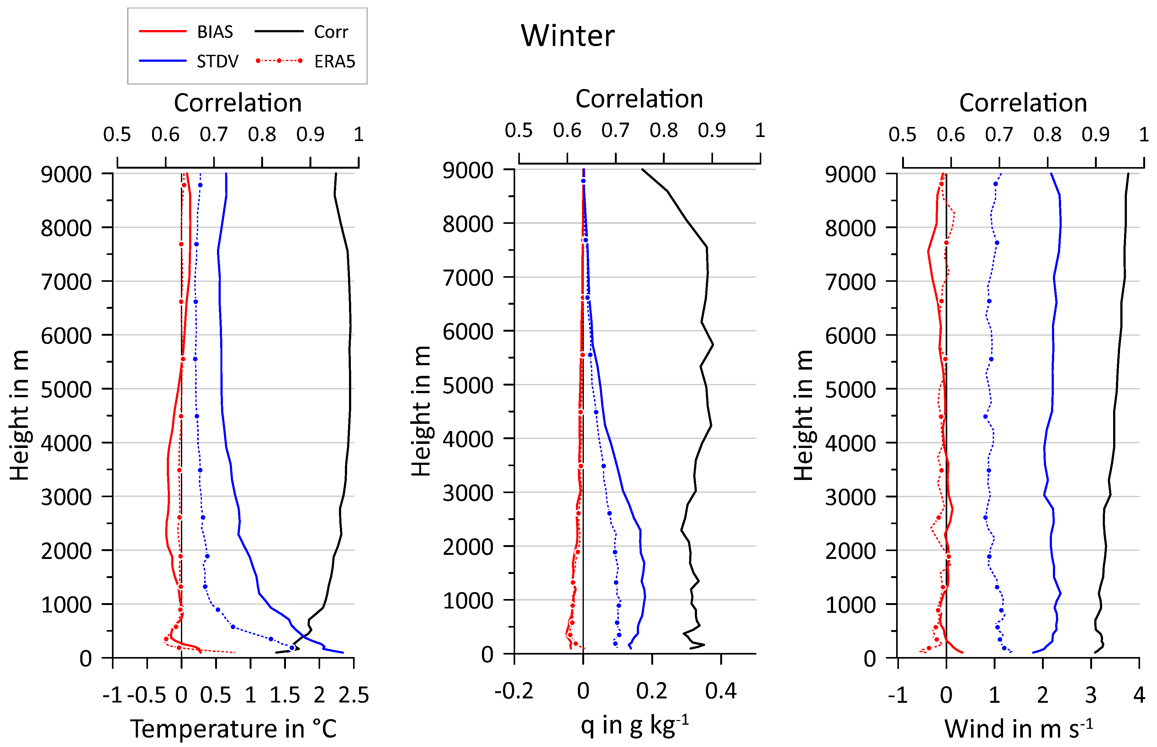
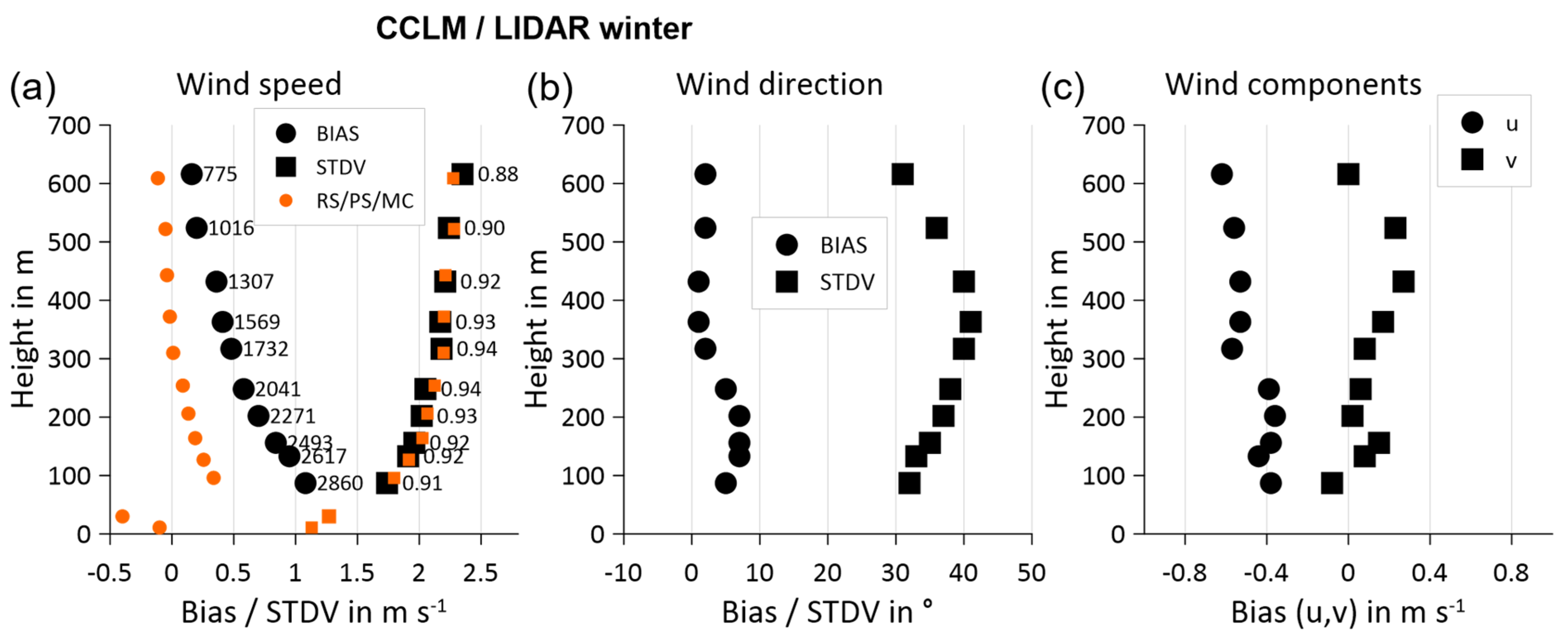
3.1.2. Statistics for Winter Months

The overall statistics of the comparisons of the C15MOD0 simulations with radiosonde profiles for the entire winter are presented in Figure 7. Altogether, 715 profiles were available. For this comparison, radiosonde data were interpolated to the model levels of the simulated profile closest to the time of the ascent. Data on each model level were linearly detrended for the calculation of correlations. Since radiosonde data are not reliable in the lowest decameters, because of flow distortion around the ship and its influence on temperature and humidity, the lowest level for the comparison was chosen as 80 m. The temperature showed very small biases of less than ±0.53 °C for all levels, while the STDV (standard deviation of the difference between model and observation) was about 2.0 °C in the lowest 500 m and less than 1.0 °C above 1000 m. The correlation was very high for all levels, with r = 0.83–0.90 in the lowest 500 m and typically 0.97 above 1000 m. The biases for wind speed were extremely small, while the STDV had values of about 2 m/s. The correlation exceeded 0.9 at all levels. For specific humidity, there was a small negative bias of −0.05 to −0.03 g/kg in the lowest 2000 m. The STDV was smaller than 0.18 g/kg, and the correlation was 0.85–0.90 below 8000 m. The decrease in the correlation above 8000 m was due to the extremely low humidity in the upper troposphere. Figure 7 also shows the bias and STDV for the comparison of ERA5 data with radiosonde data, which were assimilated in ERA5. As expected, the STDVs for ERA5 were smaller than those for CCLM. The temperature bias for ERA5 was almost zero above 1000 m, but was larger than for CCLM in the ABL.

In order to compare the C15 and C15MOD0 simulations,

Table 3. Statistics of the C15MOD0 comparison with radiosondes for layers for the winter (November–April). n = number of values, corr = correlation.

C15MOD0	Temperature °C			Spec. Humidity g/kg			Wind Speed m/s
Layer (m)	Bias	STDV	Corr	Bias	STDV	Corr	Bias	STDV	Corr	n
80–200	0.3	2.2	0.85	−0.04	0.14	0.87	0.3	1.9	0.90	2166
200–500	0.0	1.9	0.88	−0.04	0.15	0.85	0.0	2.2	0.91	3610
500–2000	−0.1	1.3	0.93	−0.03	0.18	0.86	−0.1	2.3	0.91	7942
2000–5000	−0.2	0.8	0.97	−0.01	0.11	0.87	0.0	2.1	0.93	7914
5000–8000	0.1	0.6	0.98	0.00	0.02	0.89	−0.2	2.3	0.95	4302

and

Table 4. Statistics of the C15 comparison with radiosondes for layers for the winter (November–April). n = number of values, corr = correlation.

C15	Temperature °C			Spec. Humidity g/kg			Wind Speed m/s
Layer (m)	Bias	STDV	Corr	Bias	STDV	Corr	Bias	STDV	Corr	n
80–200	−0.1	2.2	0.86	−0.05	0.13	0.88	0.3	1.9	0.90	2166
200–500	−0.2	1.9	0.87	−0.05	0.15	0.86	0.1	2.2	0.91	3610
500–2000	−0.1	1.3	0.93	−0.03	0.18	0.86	0.0	2.3	0.91	7942
2000–5000	−0.2	0.8	0.97	−0.01	0.11	0.87	0.0	2.1	0.93	7914
5000–8000	0.1	0.6	0.98	0.00	0.02	0.89	−0.2	2.3	0.95	4302

show the statistics for the layers. There were no differences between the two simulations for layers above 2000 m, indicating that the changes due to the different sea ice concentrations only appeared in the shallow ABL. This can also be seen in the comparisons between individual months (Figures S3–S6 in the Supplementary Materials). We selected the months with the largest negative and positive temperature biases at the lowest levels, that is, November and March. The overall statistics above 1000 m (Figures S3 and S5) were similar to the winter profiles shown in Figure 7. For the lowest 1000 m, there was a distinct negative temperature bias below 300 m for November (Figure S4), which was larger for C15 than for C15MOD0. This was associated with a slight improvement in the moisture bias for C15MOD0. The effect on the wind speed bias was very small. For March (Figure S6), there was a positive temperature bias below 600 m, but differences between C15 and C15MOD0 occurred only below 300 m. Ref. [26] shows that in March, there were several days with very high lead fractions, but very low surface temperatures in the leads in the MODIS observations. In these cases, the simulated surface temperature in C15MOD0 was too large, resulting in higher temperatures in the ABL compared to C15. The differences between the two runs can also be interpreted as the impact of the surface conditions on the ABL, considering that advective effects also had an impact on the conditions at the position of the Polarstern.

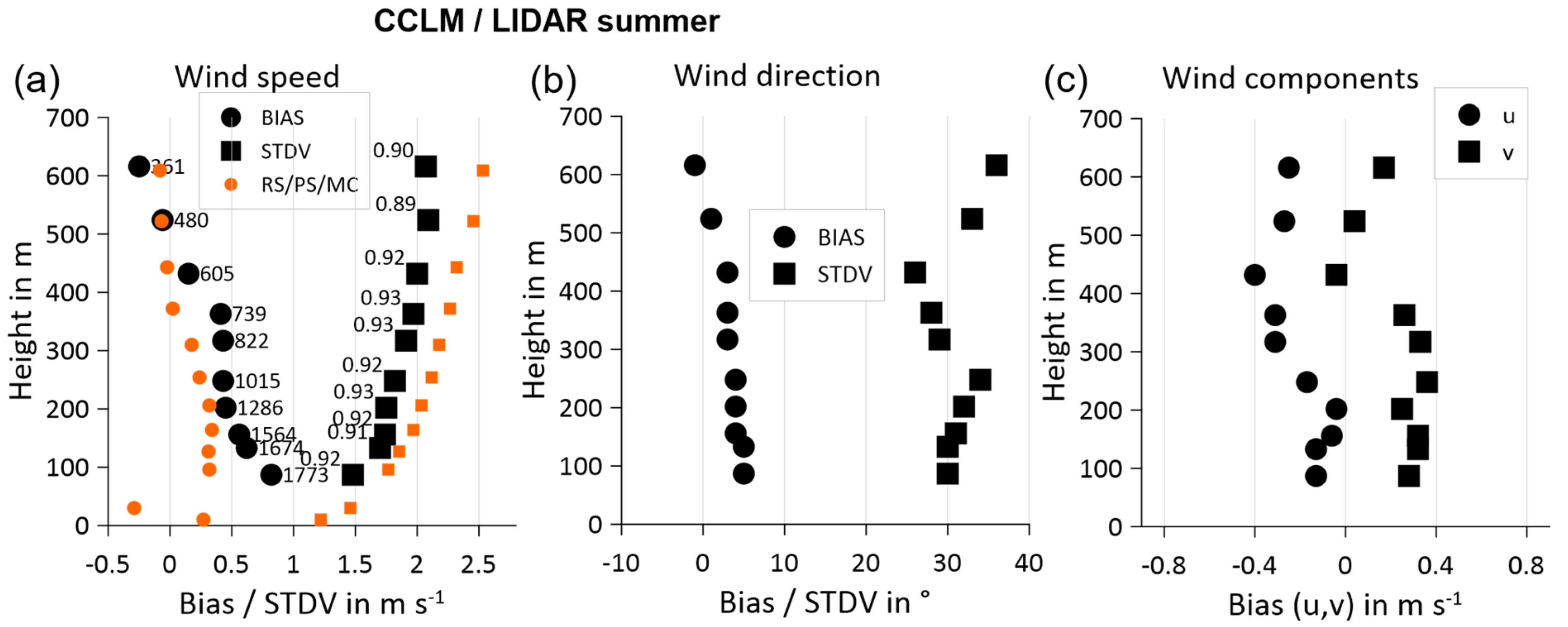
3.1.3. Statistics for Summer Months

The overall statistics of the comparisons of the C15 simulations with radiosonde profiles for the summer (May–September) are presented in Figure S7 in the Supplementary Material. Altogether, 631 profiles are available.

Table 5. Statistics of the C15 comparison with radiosondes for layers for the summer (May–September). n = number of values, corr = correlation.

C15	Temperature °C			Spec. Humidity g/kg			Wind Speed m/s
Layer (m)	Bias	STDV	Corr	Bias	STDV	Corr	Bias	STDV	Corr	n
90–200	0.3	1.8	0.72	0.02	0.36	0.84	0.3	1.9	0.88	1905
200–500	0.0	2.1	0.74	−0.01	0.44	0.83	0.1	2.2	0.87	3175
500–2000	−0.2	1.5	0.87	−0.03	0.63	0.78	−0.1	2.5	0.83	6985
2000–5000	0.1	0.9	0.95	−0.03	0.47	0.82	0.0	2.2	0.90	6976
5000–8000	0.3	0.7	0.98	−0.01	0.13	0.85	−0.2	2.5	0.94	3800

shows the corresponding statistics for the layers. There was a slight positive temperature bias in the lowest 200 m and above 4000 m. The bias for the humidity was small and comparable to that in the winter, but the STDV was much larger, particularly below 4000 m. This was caused by the much greater humidity levels in the summer. The wind speed bias was very small, and the STDV was comparable to that in the winter.

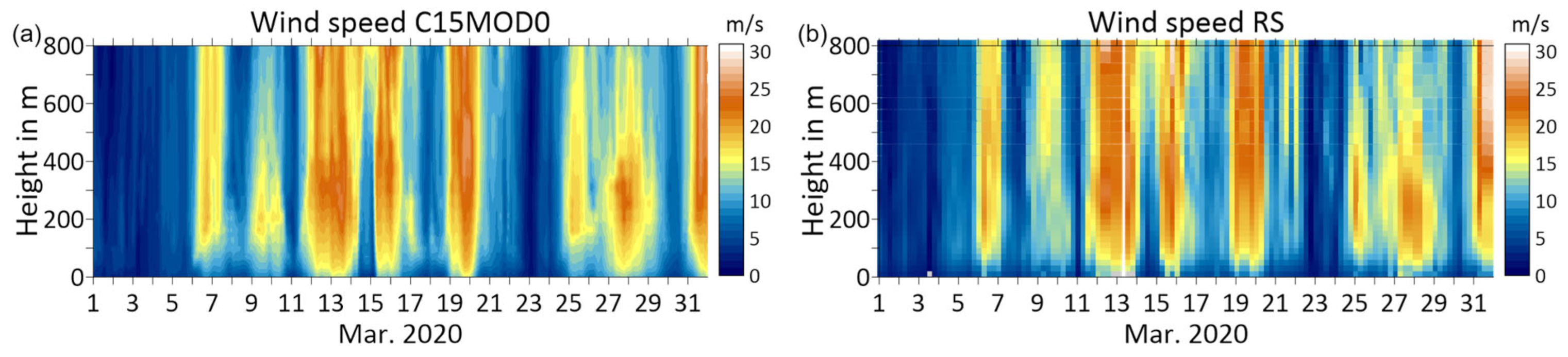
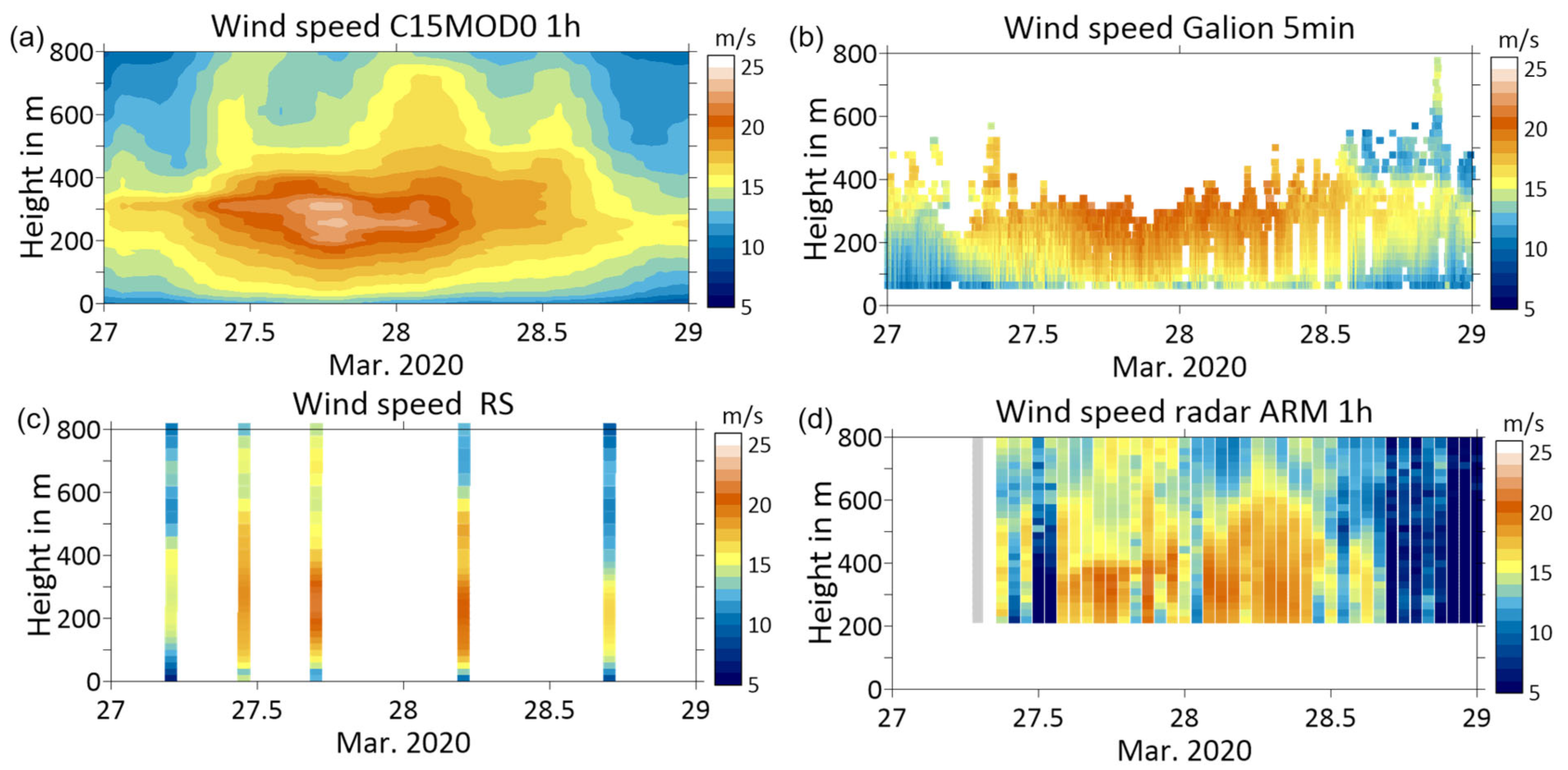
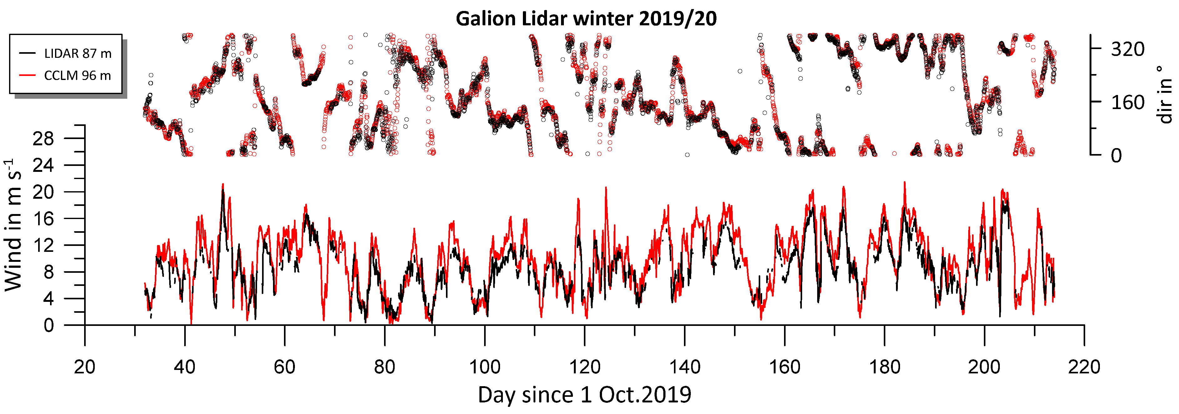
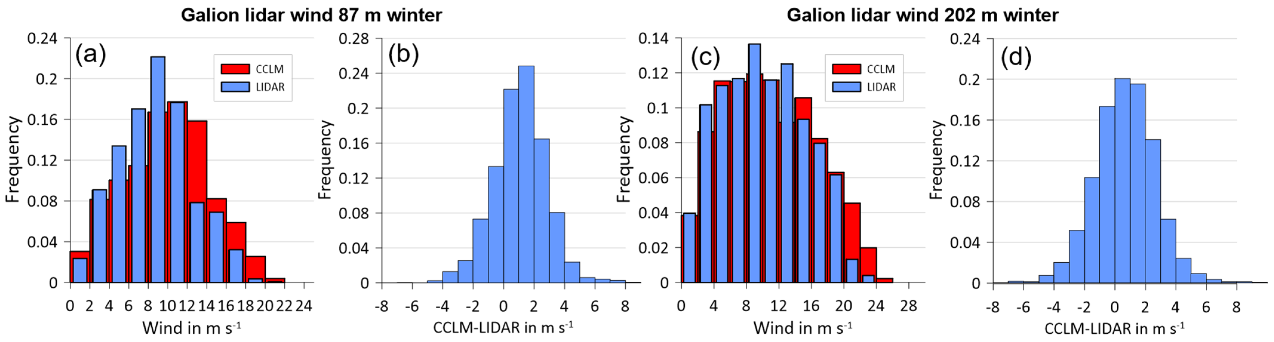
3.2. Evaluation Using Wind Lidar Data

Figure 8 shows the wind speed and wind direction at a height of about 100 m from lidar data and CCLM simulations for the entire winter period. At this height, only a few data gaps were present in the observations. The visual comparison yielded the impression that the simulations captured the observed time series very well. Some differences can be seen for the wind direction, particularly for situations with lower wind speeds. An example of these situations is shown in Figure S8 in the Supplementary Materials, which also illustrates that a phase shift between observations and simulations may lead to significant differences in the wind speed and may have contributed to the standard deviation between the two data sets. These phase shifts are presumably a result of a small position or timing bias in the model’s representation of individual weather systems.

Due to frequent gaps in the lidar data (see Figure 6b), the data at heights closest to the model levels, up to 609 m (see Table 2), were extracted as time series. The model data were then interpolated to the levels of the lidar data. The wind speed bias was at its largest at 87 m (1.1 m/s), and decreased to 0.2 m/s at higher levels (Figure 9a). At the same time, the amount of available lidar data decreased substantially with height. The number of hourly CCLM data points was 4368. While, at 87 m, the availability of lidar data was 65%, this value decreased to 30% at about 400 m and to 18% at about 600 m. The STDV increased with height from 1.7 m/s at lower levels to 2.4 m/s at about 600 m. Although the radiosonde comparisons showed almost the same values for the STDV, the bias was much lower. The lowest bias and STDV were present for near-surface measurements of the wind at about 30 m by the Polarstern meteorological system [18], and for the 10 m wind at Met City, at a distance of 300–600 m from Polarstern (see [26] for details). The positive bias at lower levels of the lidar was mainly caused by higher frequencies of wind speeds greater than 10 m/s (Figure 10a). This effect became smaller with increasing height (Figure 10c). The comparison of the wind speed distribution obtained through all simulation data with that obtained through the simulation data with available lidar data showed that there was no systematic undersampling of high wind speeds (Figure S9 in the Supplementary Material). The greater biases of the wind speed for the lidar data compared to the radiosonde data may have multiple explanations, since the lidar and radiosonde data provided very different measurements of the wind. While the lidar data represented a spatial and temporal average, the radiosonde data were single-point measurements also affected by turbulence. The impact of the ship’s superstructure on the wind field at lower levels may have also influenced the wind measurements of both systems in a different way.

Figure 9b shows the bias and STDV for the wind direction. The mean wind direction of the simulations had a small positive bias in the lowest 300 m, and this was almost zero above that level. The STDV lay between 30 and 40°. The bias for the mean wind components (Figure 9c) was negative for the u component and slightly positive for the v component.

The timeseries of the wind speed and wind direction at about 100 m height from both lidar data and CCLM simulations for the summer period (May–September) is shown in Figure S10 in the Supplementary Material. There were two large data gaps in the observations due to the breaks in the drift phases. As for the winter period, a visual comparison showed that the simulations captured the observed time series very well, but overestimated the wind speed for situations with strong winds. The bias in the wind speed profile (Figure 11a) was at its largest at 87 m (0.8 m/s), while it decreased to 0.2 m/s at about 400 m, and was slightly lower above that level. As for the winter, the amount of available lidar data decreased substantially with height. Due to the shorter period and the large gaps in the lidar data, the amount of data was much smaller compared to the winter period. Only 48% of the period was covered by lidar data at 87 m, and this value decreased to 10% at about 600 m. However, if we consider only the days with lidar measurements, the data availability is 70–80% below 200 m, greater than that for the winter. The STDV increased with height from 1.5 m/s at lower levels to 2.1 m/s at about 600 m. In contrast to the winter, the radiosonde comparisons showed larger values for the STDV, but, again, a lower bias for the lowest 200 m. The comparison with near-surface measurements showed the lowest STDV. The bias and STDV for the wind direction for the summer (Figure 11b) showed, again, a small positive bias within the lowest 400 m, and the STDV was slightly smaller, with 25–35°, than that for the winter. The bias for the mean wind components (Figure 11c) was, again, in the range of ±0.4 m/s. The lower STDV for the wind speed for summer was likely due to the fact that the mean wind speed was about 2 m/s lower than that for the winter. These differences can also be seen in the wind distributions (Figure S11 in the Supplementary Material), as we found only a few cases with wind speeds above 14 m/s at 87 m and above 16 m/s at 202 m, respectively.

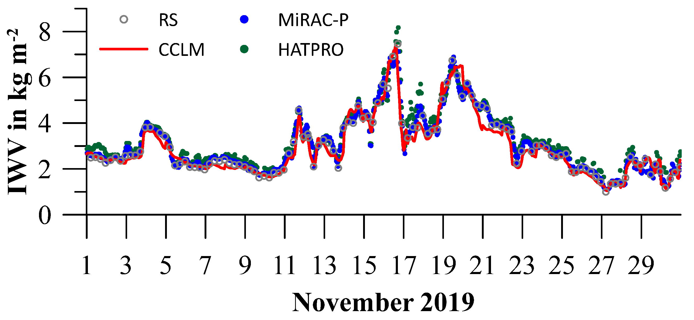
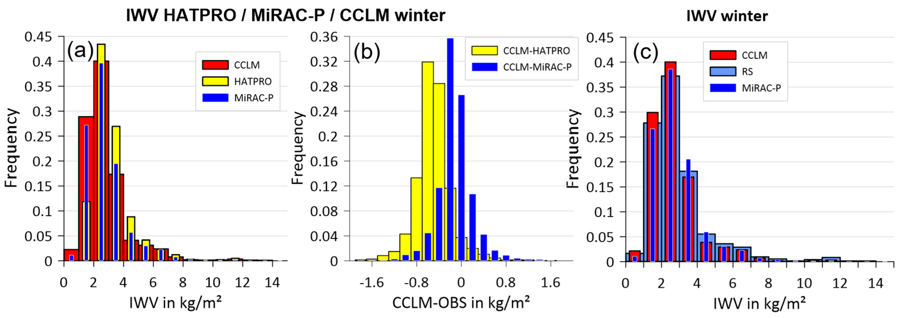
3.3. Evaluation Using Microwave Water Vapor and Temperature Radiometer Data

In contrast to radiosondes, remote sensing instruments can probe the atmosphere at a much higher temporal resolution. The integrated water vapor (IWV) retrieval of the HATPRO and MiRAC-P radiometers onboard the ship yielded IVW values every second, which were averaged to hourly values for the comparison with CCLM simulations. Figure 12 shows the HATPRO and MiRAC-P observations for November 2019 together with the CCLM simulations and data from the radiosondes. The simulations agreed very well with the observations, particularly with the radiosonde and MiRAC-P data. During periods with IWV lower than 4 g/kg, the HATPRO data showed slightly larger values. The high humidity events mid-November, as discussed above, were also obvious in the IWV data.

The frequency distributions of the IWV measurements and C15MOD0 simulations for the winter (Figure 13a) showed good agreement between CCLM and MiRAC-P, while HATPRO had lower values for IWV of less than 2 kg/m². On the other hand, the CCLM values were lower than HATPRO for IWV > 3 g/kg, while the agreement with MiRAC-P was, again, very good. This was also demonstrated in the distribution of the differences (Figure 13b). When we compared the distributions of CCLM and MiRAC-P with the IWV from radiosondes (Figure 13c), very good agreement could be observed for all IWV classes. In the summer, there were much higher IWV values than for winter. The peak of the IWV distribution occurred at 8–12 kg/m² (Figure S12a in the Supplementary Material), but 20 kg/m² was exceeded in many cases. The differences between CCLM and the observations (Figure S12b) were similar for both instruments, with a slightly broader scatter for MiRAC-P. The comparison of the IWV from radiosondes (Figure S12c) showed very good agreement for all IWV classes.

The overall statistics of the CCLM comparison with MiRAC-P and HATPRO are presented in

Table 6. Statistics of the CCLM comparison with observations (OBS) for the IWV from MiRAC-P and HATPRO, as well as the mean temperature from HATPRO of the lowest 2 km (T2 km) for the winter (November–April, 11-04, C15MOD0) and the summer (May–September, 05-09, C15). N = number of values, corr = correlation.

Period	Instrument	Quantity	n	OBS	CCLM	Bias	STDV	Corr.
11-04	MiRAC-P	IWV in kg/m2	4305	2.8	2.7	−0.1	0.3	0.97
11-04	HATPRO	IWV in kg/m2	4107	3.2	2.7	−0.5	0.3	0.98
05-09	MiRAC-P	IWV in kg/m2	3540	12.2	12.3	0.1	1.6	0.96
05-09	HATPRO	IWV in kg/m2	3539	12.1	12.3	0.2	1.2	0.98
11-04	HATPRO	T2 km in °C	7379	−21.2	−20.3	0.9	1.5	0.97
05-09	HATPRO	T2 km in °C	6922	−2.1	−2.2	−0.1	1.1	0.98

. For the IWV, there were only a few gaps in the hourly data of the measurements, and the data availability was between 94 and 99%. The bias of CCLM compared to HATPRO was −0.5 kg/m² for the winter, while it was only −0.1 kg/m² compared to MiRAC-P. The STDV was 0.3 kg/m² for both data sets. For the summer period, the IWV was around 12 kg/m², and the bias of CCLM was slightly positive. The STDV for the comparison with MiRAC-P was larger than that for HATPRO. These findings are consistent with [24], who observed a better performance of MiRAC-P compared to radiosondes for low IWV values and a larger scatter of MiRAC-P than HATPRO for larger IWV values. In addition to IWV, we compared the mean temperature of the lowest 2 km from HATPRO with the simulations (note that half-hourly data were used; thus, the amount of data was larger). There was a warm bias of 0.9 °C for the winter, while the bias was small for the summer (−0.1 °C). The correlation coefficients (detrended data) were very high for all seasons and quantities.

4. Discussion

Radiosondes, during the MOSAiC experiment, have been launched every 3–6 h for a full year over sea ice in the Arctic, which is an unprecedented data set representing a backbone for model verification for the ABL and the whole troposphere. However, the lowest 100 m of a radiosonde’s ascent is problematic, particularly due to the wind profile, since errors occur via the pendulum motion of the radiosonde directly after the start, and the balloon has to adapt to the ambient wind speed. In addition, the wind field at lower levels is disturbed by the ship’s superstructure. Despite the relatively high temporal resolution, the radiosonde data often fail to resolve the development of mesoscale events such as LLJs. The comparison of CCLM simulations with radiosonde data showed very good agreement for the ABL and the whole troposphere for the winter months. The biases for wind speed were extremely low (less than 0.3 m/s), while the STDV had values of about 2 m/s. In the study cited in [10], which compared CCLM with radiosonde data over thick ice in the inner Arctic for April 2019 [34], a larger bias of −1 m/s was found for the lower 1000 m and above 5000 m. Comparisons of RCMs with radiosondes for the SHEBA campaign 1997–1998 [13] were performed in [16]. They found large biases of ±2 °C for the temperature below 1 km, indicating problems with the ABL parameterizations of the models. The wind speed biases were at their greatest close to the surface (−2 to +4 m/s), but were also large in the lowest 4000 m (±2 m/s). Comparisons of eight RCMs for the SHEBA period were presented in [35]. This study found differences between the coldest and warmest model of 4–5 °C in the lower troposphere, which decreased to 0.5–1.0 °C at 500 hPa. The study in [8] compared several RCMs, including CCLM, for summer 2014 over the Arctic ocean, and found slightly negative biases of −0.2 °C for the temperature and an RMSE (root mean square error) of around 1 °C throughout the entire troposphere in most models (for these small biases RMSE is almost identical to STDV). The smaller RMSE/STDV compared to the STDV for the temperature in our study can be explained by the fact that the comparison was made for a homogeneous ocean environment. The study cited in [7], conducted in the marginal ice zone using the same set of models as [8] for late summer 2014, showed comparable differences to our present study for the tropospheric temperature. For specific humidity, we found a low negative bias of about −0.04 g/kg in the lower troposphere for winter. For the summer period, the bias was smaller (−0.03 g/kg), but the STDV was larger due to the higher levels of humidity (maxima of 0.63 g/kg and 0.18 g/kg in the 500–2000 m layer for summer and winter, respectively). The humidity bias in the lower troposphere for summer was much smaller than that in the comparison studies of [8] and [7], where the bias varied between −0.3 and +0.2 g/kg for the different RCMs.

In contrast to radiosondes, ground-based remote sensing instruments can probe the atmosphere at a much higher temporal resolution. Herein, we used wind lidar, wind radar, and measurements of IWV and temperatures in the lower troposphere by microwave radiometers for a comparison on an hourly time scale. The radar wind profiles were found to be unsuitable for model evaluation at the present stage. In contrast, the lidar wind profiles had many gaps, but represented a valuable data set for model evaluation. Ship-based wind lidar data have rarely been used in polar regions for model comparisons. One example was shown for the Antarctic in [30], where lidar wind was compared to CCLM for a five-week period during the austral summer in the southern Weddell Sea. They found a very small bias for the wind speed (±0.1 m/s) and an RMSE of around 2 m/s. For wind direction, there was a small bias of −5° and an RMSE of 30°. While the latter was comparable with the present study, the wind speed bias compared to the wind lidar was much greater in the present study, particularly for the winter. Future evaluations using the data of two other wind lidars during MOSAiC [12] are planned.

Comparisons with HATPRO/MiRAC-P IWV showed very good agreement. HATPRO overestimated IWV for the winter, but MiRAC-P data fit well to the radiosondes and the simulations. For the summer, the simulations agreed well with data of both instruments, but the scatter for MiRAC-P data was larger. These results are consistent with [24], who found a better performance of MiRAC-P compared to radiosondes for low IWV values and a larger scatter of MiRAC-P than HATPRO for greater IWV values. The comparison of the simulations with HATPRO temperature for the lowest 2 km showed a very good agreement.

The good performance of CCLM in representing the vertical structure of the Arctic troposphere resulted partly from the fact that the simulations were initialized daily with ERA5 data, where radiosonde data from Polarstern were assimilated. This kind of model setup was also used in recent RCM intercomparison studies in the frame of the Arctic CORDEX (COordinated Regional Downscaling Experiment) initiative, where RCMs were initialized by and nudged to large-scale reanalyses in order to obtain insight into the shortcomings of model physics by comparisons to other observations [7,8]. However, the studies of [8] and [7] showed that ERA data also had biases compared to radiosondes, which were in the same range as for RCMs, but STDVs for ERA were smaller than those for RCMs. For summer conditions in the central Arctic, the authors of [9] found a warm bias of up to 0.5–0.9 °C for the operational ECMWF model in the lowest 500 m, which changed to a negative bias of almost −1 °C at 1 km. In the present study, the STDVs of ERA5 data were substantially smaller than for CCLM. This may have resulted from the high frequency of radiosonde launches during MOSAiC. It must also be noted that the CCLM simulations used ERA5 data only at the lateral boundaries, without nudging during the simulation time of 30 h. Due to the large domain of the model, different developments of, e.g., cyclones and mesoscale features can occur compared to ERA5. Differences also occur because of the different parameterizations of the models, particularly for sea ice and cloud parameterizations [8,26]. Since ERA5 uses a fixed sea ice thickness without snow cover, a distinct warm bias for the near-surface temperature of about 2.5 °C and an underestimation of the temperature variability was found by [26] for the winter period at the Polarstern’s position. The recent study of [36] using the MODIS ice surface temperature showed a warm bias for the surface temperature of 6.0 °C for radiatively clear situations at the Polarstern’s position for the winter of 2019/20. The runs of the present study with different sea ice data (C15 and C15MOD0) indicated that the representation of sea ice leads affects the lower tropospheric structure in the lowest 300 m, that is, the ABL. The main effect was found for the temperature, while the wind structure was only slightly modified.

Future work will include simulations with higher resolutions, extending down to 1 km, with a focus on the direct impact of sea ice leads on the ABL. Studies of LLJs, as well as intercomparisons with other RCMs in the frame of the Arctic CORDEX, will also be included.

References

1. Hansen, J.E.; Ruedy, R.; Sato, M.; Lo, K. Global surface temperature change. Rev. Geophys. 2010, 48, RG4004. [Google Scholar] [CrossRef] [Green Version]
2. Rantanen, M.; Karpechko, A.Y.; Lipponen, A.; Nordling, K.; Hyvärinen, O.; Ruosteenoja, K.; Vihma, T.; Laaksonen, A. The Arctic has warmed nearly four times faster than the globe since 1979. Commun. Earth Environ. 2022, 3, 168. [Google Scholar] [CrossRef]
3. Wendisch, M.; Brückner, M.; Crewell, S.; Ehrlich, A.; Notholt, J.; Lüpkes, C.; Macke, A.; Burrows, J.P.; Rinke, A.; Quaas, J.; et al. Atmospheric and Surface Processes, and Feedback Mechanisms Determining Arctic Amplification: A Review of First Results and Prospects of the (AC)3 Project. Bull. Am. Meteorol. Soc. 2023, 104, E208–E242. [Google Scholar] [CrossRef]
4. Kohnemann, S.H.E.; Heinemann, G.; Bromwich, D.H.; Gutjahr, O. Extreme Warming in the Kara Sea and Barents Sea during the Winter Period 2000. J. Clim. 2017, 30, 8913–8927. [Google Scholar] [CrossRef] [Green Version]
5. Duvivier, A.K.; Cassano, J.J. Evaluation of WRF Model Resolution on Simulated Mesoscale Winds and Surface Fluxes near Greenland. Mon. Weather. Rev. 2013, 141, 941–963. [Google Scholar] [CrossRef]
6. Gutjahr, O.; Heinemann, G. A model-based comparison of extreme winds in the Arctic and around Greenland. Int. J. Clim. 2018, 38, 5272–5292. [Google Scholar] [CrossRef] [Green Version]
7. Sedlar, J.; Tjernström, M.; Rinke, A.; Orr, A.; Cassano, J.; Fettweis, X.; Heinemann, G.; Seefeldt, M.; Solomon, A.; Matthes, H.; et al. Confronting Arctic Troposphere, Clouds, and Surface Energy Budget Representations in Regional Climate Models with Observations. J. Geophys. Res. Atmos. 2020, 125, e2019JD031783. [Google Scholar] [CrossRef]
8. Inoue, J.; Sato, K.; Rinke, A.; Cassano, J.J.; Fettweis, X.; Heinemann, G.; Matthes, H.; Orr, A.; Phillips, T.; Seefeldt, M.; et al. Clouds and Radiation Processes in Regional Climate Models Evaluated Using Observations Over the Ice-free Arctic Ocean. J. Geophys. Res. Atmos. 2020, 126, e2020JD033904. [Google Scholar] [CrossRef]
9. Tjernström, M.; Svensson, G.; Magnusson, L.; Brooks, I.M.; Prytherch, J.; Vüllers, J.; Young, G. Central Arctic weather forecasting: Confronting the ECMWF IFS with observations from the Arctic Ocean 2018 expedition. Q. J. R. Meteorol. Soc. 2021, 147, 1278–1299. [Google Scholar] [CrossRef]
10. Heinemann, G.; Willmes, S.; Schefczyk, L.; Makshtas, A.; Kustov, V.; Makhotina, I. Observations and Simulations of Meteorological Conditions over Arctic Thick Sea Ice in Late Winter During the Transarktika 2019 Expedition. Atmosphere 2021, 12, 174. [Google Scholar] [CrossRef]
11. Heinemann, G.; Drüe, C.; Makshtas, A. A Three-Year Climatology of the Wind Field Structure at Cape Baranova (Severnaya Zemlya, Siberia) from SODAR Observations and High-Resolution Regional Climate Model Simulations during YOPP. Atmosphere 2022, 13, 957. [Google Scholar] [CrossRef]
12. Shupe, M.D.; Rex, M.; Blomquist, B.; Persson, P.O.G.; Schmale, J.; Uttal, T.; Althausen, D.; Angot, H.; Archer, S.; Bariteau, L.; et al. Overview of the MOSAiC expedition: Atmosphere. Elementa: Sci. Anthr. 2022, 10, 00060. [Google Scholar] [CrossRef]
13. Uttal, T.; Curry, J.A.; Mcphee, M.G.; Perovich, D.K.; Moritz, R.E.; Maslanik, J.A.; Guest, P.S.; Stern, H.L.; Moore, J.A.; Turenne, R.; et al. Surface Heat Budget of the Arctic Ocean. Bull. Am. Meteorol. Soc. 2002, 83, 255–275. [Google Scholar] [CrossRef]
14. Graham, R.M.; Rinke, A.; Cohen, L.; Hudson, S.R.; Walden, V.P.; Granskog, M.A.; Dorn, W.; Kayser, M.; Maturilli, M. A comparison of the two Arctic atmospheric winter states observed during N-ICE2015 and SHEBA. J. Geophys. Res. Atmos. 2017, 122, 5716–5737. [Google Scholar] [CrossRef]
15. Wyser, K.; Jones, C.G. Modeled and observed clouds during Surface Heat Budget of the Arctic Ocean (SHEBA). J. Geophys. Res. Atmos. 2005, 110, D09207. [Google Scholar] [CrossRef] [Green Version]
16. Tjernström, M.; Žagar, M.; Svensson, G.; Cassano, J.J.; Pfeifer, S.; Rinke, A.; Wyser, K.; Dethloff, K.; Jones, C.; Semmler, T.; et al. ‘Modelling the Arctic Boundary Layer: An Evaluation of Six Arcmip Regional-Scale Models using Data from the Sheba Project’. Bound. -Layer Meteorol. 2005, 117, 337–381. [Google Scholar] [CrossRef]
17. Maturilli, M.; Sommer, M.; Holdridge, D.J.; Dahlke, S.; Graeser, J.; Sommerfeld, A.; Jaiser, R.; Deckelmann, H.; Schulz, A. MOSAiC Radiosonde Data (Level 3). 2022. Available online: https://doi.pangaea.de/10.1594/PANGAEA.943870 (accessed on 26 October 2022).
18. Knust, R. Polar Research and Supply Vessel POLARSTERN operated by the Alfred-Wegener-Institute. J. Large-Scale Res. Facil. JLSRF 2017, 3, 119. [Google Scholar] [CrossRef]
19. Vaisala. Vaisala Radiosonde RS41 Measurement Performance. Available online: https://www.vaisala.com/sites/default/files/documents/White%20paper%20RS41%20Performance%20B211356EN-A.pdf (accessed on 18 May 2023).
20. Dirksen, R.J.; Sommer, M.; Immler, F.J.; Hurst, D.F.; Kivi, R.; Vömel, H. Reference quality upper-air measurements: GRUAN data processing for the Vaisala RS92 radiosonde. Atmos. Meas. Tech. 2014, 7, 4463–4490. [Google Scholar] [CrossRef] [Green Version]
21. Brooks, I.M. MOSAiC: Wind Profiles from Galion G4000 Lidar Wind Profiler—Version 2. 2022. Available online: https://catalogue.ceda.ac.uk/uuid/c4abd037c7ad4019ad02d0c802e2f27e (accessed on 19 October 2022).
22. Newsom, R.K.; Brewer, W.A.; Wilczak, J.M.; Wolfe, D.E.; Oncley, S.P.; Lundquist, J.K. Validating precision estimates in horizontal wind measurements from a Doppler lidar. Atmos. Meas. Tech. 2017, 10, 1229–1240. [Google Scholar] [CrossRef] [Green Version]
23. Martin, T.; Muradyan, P.; Coulter, R. ARM: 1290-MHz Beam-Steered Radar Wind Profiler: Wind and Moment Averages. 2012. Available online: https://www.osti.gov/dataexplorer/biblio/dataset/1095573 (accessed on 25 October 2022).
24. Walbröl, A.; Crewell, S.; Engelmann, R.; Orlandi, E.; Griesche, H.; Radenz, M.; Hofer, J.; Althausen, D.; Maturilli, M.; Ebell, K. Atmospheric temperature, water vapour and liquid water path from two microwave radiometers during MOSAiC. Sci. Data 2022, 9, 534. [Google Scholar] [CrossRef]
25. Cox, C.; Gallagher, M.; Shupe, M.; Persson, O.; Solomon, A.; Blomquist, B.; Brooks, I.; Costa, D.; Gottas, D.; Hutchings, J.; et al. 10-meter (m) meteorological flux tower measurements (Level 1 Raw), Multidisciplinary Drifting Observatory for the Study of Arctic Climate (MOSAiC), central Arctic, October 2019–September 2020. 2021. Available online: https://arcticdata.io/catalog/view/doi%3A10.18739%2FA2VM42Z5F (accessed on 5 November 2021).
26. Heinemann, G.; Schefczyk, L.; Willmes, S.; Shupe, M.D. Evaluation of simulations of near-surface variables using the regional climate model CCLM for the MOSAiC winter period. Elem. Sci. Anthr. 2022, 10, 00033. [Google Scholar] [CrossRef]
27. Ebell, K.; Walbröl, A.; Engelmann, R.; Griesche, H.; Radenz, M.; Hofer, J.; Althausen, D. Temperature and Humidity Profiles, Integrated Water Vapour and Liquid Water Path Derived from the HATPRO Microwave Radiometer Onboard the Polarstern during the MOSAiC Expedition. 2022. Available online: https://doi.pangaea.de/10.1594/PANGAEA.941389 (accessed on 24 October 2022).
28. Walbröl, A.; Orlandi, E.; Crewell, S.; Ebell, K. Integrated Water Vapour Derived from the MiRAC-P Microwave Radiometer Onboard the Polarstern during the MOSAiC Expedition. 2022. Available online: https://doi.pangaea.de/10.1594/PANGAEA.941470 (accessed on 24 October 2022).
29. Hersbach, H.; Bell, B.; Berrisford, P.; Hirahara, S.; Horányi, A.; Muñoz-Sabater, J.; Nicolas, J.; Peubey, C.; Radu, R.; Schepers, D.; et al. The ERA5 global reanalysis. Q. J. R. Meteorol. Soc. 2020, 146, 1999–2049. [Google Scholar] [CrossRef]
30. Zentek, R.; Heinemann, G. Verification of the regional atmospheric model CCLM v5.0 with conventional data and lidar measurements in Antarctica. Geosci. Model Dev. 2020, 13, 1809–1825. [Google Scholar] [CrossRef] [Green Version]
31. Heinemann, G. Assessment of Regional Climate Model Simulations of the Katabatic Boundary Layer Structure over Greenland. Atmosphere 2020, 11, 571. [Google Scholar] [CrossRef]
32. Spreen, G.; Kaleschke, L.; Heygster, G. Sea ice remote sensing using AMSR-E 89-GHz channels. J. Geophys. Res. Atmos. 2008, 113, C02S03. [Google Scholar] [CrossRef] [Green Version]
33. Zhang, J.; Rothrock, D.A. Modeling Global Sea Ice with a Thickness and Enthalpy Distribution Model in Generalized Curvi-linear Coordinates. Mon. Wea. Rev. 2003, 131, 845–861. [Google Scholar] [CrossRef]
34. Frolov, I.E.; Ivanov, V.V.; Filchuk, K.V.; Makshtas, A.P.; Kustov, V.Y.; Mahotina, I.A.; Ivanov, B.V.; Urazgildeeva, A.V.; Syoemin, V.L.; Zimina, O.L.; et al. Transarktika-2019: Winter expedition in the Arctic Ocean on the R/V “Akademik Tryoshnikov”. Arct. Antarct. Res. 2019, 65, 255–274. [Google Scholar] [CrossRef] [Green Version]
35. Rinke, A.; Dethloff, K.; Cassano, J.J.; Christensen, J.H.; Curry, J.A.; Du, P.; Girard, E.; Haugen, J.-E.; Jacob, D.; Jones, C.G.; et al. Evaluation of an ensemble of Arctic regional climate models: Spatiotemporal fields during the SHEBA year. Clim. Dyn. 2006, 26, 459–472. [Google Scholar] [CrossRef]
36. Herrmannsdörfer, L.; Müller, M.; Shupe, M.D.; Rostosky, P. Surface temperature comparison of the Arctic winter MOSAiC observations, ERA5 reanalysis, and MODIS satellite retrieval. Elem. Sci. Anthr. 2023, 11, 00085. [Google Scholar] [CrossRef]
37. Heinemann, G. Regional Climate Model Simulations (CCLM 15km) of Near-Surface Variables for the MOSAiC Winter Period. 2022. Available online: https://doi.pangaea.de/10.1594/PANGAEA.944502 (accessed on 24 March 2023).
38. Heinemann, G. Regional Climate Model Simulations (CCLM 15km) of Profiles for the MOSAiC Period. 2023. Available online: https://zenodo.org/record/7756964 (accessed on 24 March 2023).
39. Nixdorf, U.; Dethloff, K.; Rex, M.; Shupe, M.; Sommerfeld, A.; Perovich, D.K.; Nicolaus, M.; Heuzé, C.; Rabe, B.; Loose, B.; et al. MOSAiC Extended Acknowledgement. 2021. Available online: https://zenodo.org/record/5541624 (accessed on 24 March 2023).
Figure 1. CCLM model domain with 14 km resolution (a) (Arctic circle as blue dashed line) and subdomain showing the drift track (b), with topography and AMSR2 sea ice concentration, for 23 April 2020. The green line shows the entire track of Polarstern, and the three drift phases are marked in blue, light blue, and orange. Dates of ship positions at the start and end of the drift phases are marked.
Meteorology 02 00016 g001
Figure 2. Profiles of the temperature, wind speed, wind direction, and specific humidity (panels from left to right) for 0500 UTC on 1 March 2020 for radiosonde data (black line) and the C15MOD0 simulation (red line).
Meteorology 02 00016 g002
Figure 3. Time–height cross-sections for the temperature from C15MOD0 simulations (a) and radiosondes (c), and for the specific humidity from simulations (b) and radiosondes (d) for 1–30 November 2019. Interpolated fields are shown for the simulations, while radiosonde data are shown as pixels.
Meteorology 02 00016 g003
Figure 4. Time–height cross-sections for the wind speed from C15MOD0 simulations (a) and radiosondes (c), and for the wind direction from simulations (b) and radiosondes (d) for 1–30 November 2019. Interpolated fields are shown for the simulations, while radiosonde data are shown as pixels.
Meteorology 02 00016 g004
Figure 5. Time–height cross-sections for the wind speed from C15MOD0 simulations (a) and radiosondes (b) for 1–31 March 2020. Interpolated fields are shown for the simulations, while radiosonde data are shown as pixels.
Meteorology 02 00016 g005
Figure 6. Time–height cross-sections for the wind speed for 27–28 March 2020 from C15MOD0 simulations (a), Galion wind lidar (b), radiosondes (c), and wind radar (d). Interpolated fields are shown for the simulations, while observations are shown as pixels. Missing data are white; data with NA values are grey.
Meteorology 02 00016 g006
Figure 7. Profiles of bias (red lines), STDV (blue lines), and correlation (black lines) for the comparison of C15MOD0 simulations with radiosondes for temperature (left), specific humidity (middle), and wind speed (right) for November 2019–April 2020 (715 profiles). Bias and STDV for the comparison of ERA5 with radiosonde data are shown as dotted lines with symbols.
Meteorology 02 00016 g007
Figure 8. Hourly mean values of the wind speed (lower panel) and wind direction (upper panel) for 1 November 2019 to 30 April 2020 for lidar measurements at a height of 87 m (black) and C15MOD0 simulations at a height of 96 m (red).
Meteorology 02 00016 g008
Figure 9. Bias (CCLM-OBS) and STDV for the comparison of wind from the Galion lidar (black symbols) and C15MOD0 simulations at different heights for the winter period, based on hourly data. (a) Bias (black dots) and STDV (black squares) for the wind speed (correlation coefficients (detrended data) are shown as labels on the STDV data, and numbers of data points are shown as labels on the bias data). The bias and STDV for the comparison with radiosondes (RS), the wind at 30 m from the Polarstern (PS) measurements, and the 10 m wind at Met City (MC) are shown as orange symbols. (b) Bias (black dots) and STDV (black squares) for the wind direction; (c) biases for the wind components (dots for u and squares for v).
Meteorology 02 00016 g009
Figure 10. Frequency distributions of the Galion wind lidar measurements and C15MOD0 simulated wind speed (1 h values) at 87 m (a) and 202 m (c), and their differences at 87 m (b) and 202 m (d), for the whole winter.
Meteorology 02 00016 g010
Figure 11. Bias (CCLM-OBS) and STDV for the comparison of wind from lidar (black symbols) and C15 simulations at different heights for the summer (May–September), based on hourly data. (a) Bias (black dots) and STDV (black squares) for the wind speed (correlation coefficients (detrended data) are shown as labels on the STDV data; numbers of data points are shown as labels on the bias data). The bias and STDV for the comparison with radiosondes (RS), the wind at 30 m from Polarstern (PS) measurements, and the 10 m wind at Met City (MC) are shown as orange symbols. (b) Bias (black dots) and STDV (black squares) for the wind direction; (c) biases for the wind components (dots for u and squares for v).
Meteorology 02 00016 g011
Figure 12. Integrated water vapor (IWV) from radiosonde data (grey circles), HATPRO data (green dots), MiRAC-P data (blue dots), and C15MOD0 simulations (red line) for November 2019.
Meteorology 02 00016 g012
Figure 13. (a) Frequency distributions of IWV measurements (HATPRO yellow, MiRAC-P dark blue) and C15MOD0 simulations (red) for the winter period (1 h values); (b) frequency distributions of the differences; (c) frequency distributions of IWV from radiosondes (RS light blue), MiRAC-P (dark blue), and C15MOD0 simulations (red).
Meteorology 02 00016 g013