Initial-Value vs. Model-Induced Forecast Error: A New Perspective

Abstract

Numerical models of the atmosphere are based on the best theory available. Understandably, the theoretical assessment of errors induced by the use of such models is confounding. Without clear theoretical guidance, the experimental separation of the model-induced part of the total forecast error is also challenging. In this study, the forecast error and ensemble perturbation variances were decomposed. Smaller- and larger-scale components, separated as a function of the lead time, were independent. They were associated with features with completely vs. only partially lost skill, respectively. For their phenomenological description, the larger-scale variance was further decomposed orthogonally into positional and structural components. An analysis of the various components revealed that chaotically amplifying initial perturbation and error predominantly led to positional differences in forecasts, while structural differences were interpreted as an indicator of the model-induced error. Model-induced errors were found to be relatively small. These results confirmed earlier assumptions and limited empirical evidence that numerical models of the atmosphere may be near perfect on the scales they well resolve.

1. Introduction

Forecast error originates from two sources: error in the initial condition, and error in model formulation, including errors due to the discontinuous representation of nature in numerical models [1]. The chaotic evolution of initial errors was extensively studied, often using ensemble perturbations (e.g., [2,3,4,5,6]). Model-induced perturbations are harder to understand or reproduce (e.g., [7,8,9]). No single mechanism or generally accepted explanation has been proposed; model-related errors likely have multiple sources [10]. From perturbed ensemble forecasts replicating much of the divergence between reality and its best forecast, one may surmise that at least in the extratropics, the bulk of the total forecast error may be related to the initial value.

Though the two sources of error are undisputed, they lack clear theoretical guidance, and thus, their empirical separation remains a challenge. In the total error, the two components are inherently mixed and possibly convoluted (e.g., [11]). Partly due to this lack of empirical separation, some confusion about the sources of forecast error remains. This confusion is exemplified by the common practice of forecast error being referred to as “model error”, as if all or most of the forecast error originates from the use of imperfect models. While it is true that most weather forecasts originate from numerical models, the bulk of extratropical forecast error can be traced back to initial value uncertainty, which is amplified due to the chaotic nature of the atmosphere (see, e.g., [12,13,14]). Model deficiencies appear to play a lesser role. If indeed extratropical forecast error is dominated by initial-value-related uncertainty, a clear distinction between the two error sources is needed. Quantitatively, how much of the error is model- vs. initial-condition-induced?

Skill and error are inverse metrics of forecast performance. In this study, we explored some aspects of the growth of error or loss of skill in weather forecasts. In Section 2, we review the well-known dependence of forecast skill on the scale of weather features. First, we assess the lead time where practically all skill is lost as a function of the scale of weather features. In Section 3, we describe the methodology and data used for a phenomenological study of the loss of skill. Section 4 explores whether skill is lost more due to the displacement or structural distortion of forecast weather features. The loss of skill is also compared with the divergence among initially similar ensemble members. Error and ensemble perturbation components are compared and interpreted in terms of model- and initial-value-induced error variance in Section 5, while a summary is offered in Section 6.

2. Skill and Scale

2.1. Error and Skill

An error field $e_i$in an NWP forecast $F_i$ of lead time $i$ is usually defined as its difference from the proxy for truth (typically an NWP analysis field $T$), which are both given on the grid of a model and valid at the same time:

$$e_i=F_i-T$$

(1)

The root-mean-square error (rmse, $d_i$) and its square (variance error [15]; the systematic error is assumed to be small, and thus, henceforth, the variance error and error variance are used interchangeably as $d_i^2$) are two simple and widely used metrics for the quantification of error:

$$d_i=\sqrt{{{\displaystyle \sum }}_{j=1}^n{e}_{i,j}^2/n}$$

(2)

where $e_{i,j}$ is the error at grid $j$ of $e_i$ and $n$ is the number of grid points. Obviously, the error field ($e_i$) is unknown until the verifying data becomes available. The error variance, however, can be estimated either statistically or as the spread of dynamically generated ensembles [1,16,17]. The error variance can be conveniently standardized using the natural variability of the system, i.e., $d_i^2/V$, where $V$ is the climatic variance.

As mentioned above, the forecast error is attributed to two sources: the initial error, which is amplified chaotically [18,19], and imperfect model formulation [7,20]. Leith [21], Kleeman [22], and Zhou and Toth [23] argued that NWP models can be considered as a near-perfect representation of larger-scale processes in the atmosphere. Lorenz [24] suggested that the chaotic growth of initial error variance can be described using a logistic relationship, which Feng et al. [12] converted into the following form:

$$d_i^2=R·c/\left(e^{-\alpha ·i·\mathsf{\Delta }t}+c\right)$$

(3a)

$$c=d_0^2/\left(R-d_0^2\right)$$

(3b)

where $d_0^2$ is the initial error variance, $d_i^2$ is the forecast error variance at lead time $i·\mathsf{\Delta }t$, $R$ is the range between the lower and upper saturation value, and $\alpha$ is the exponential growth rate.

The exponential growth factor $\alpha$ reflects how unstable a dynamical system is [14,15]. Due to the divergence of initially close-by trajectory segments, with increasing lead time, the forecast retains less and less information about the future weather, eventually becoming like a random draw from the climatic distribution. The expected error variance beyond this lead time equals the distance between two randomly chosen states, which is twice the climatic variance:

$$R=2V$$

(4)

R is also called the saturation level of the forecast error and is related to the size of the natural system [25]. When the error in a forecast approaches this level, it is an indication that it nears its limit of useful skill.

More formally, skill scores are positively oriented metrics of forecast performance, with 1 and 0 indicating perfect and no skill, respectively. While the rms or variance error can be considered inverse indicators of forecast skill, correlation metrics, such as the pattern anomaly correlation (PAC) is a direct measure of skill:

$$r_i=\frac{\left(F_i-C\right)\left(T-C\right)}{\left|F_i-C\right|·\left|T-C\right|}$$

(5)

where $C$ is the climatic mean and $\left|·\right|$ denotes the commonly used L2 norm [26]. As is well known, the square of the PAC quantifies the fraction of the observed anomaly (taken from the climatic mean) variance explained by the forecast [27], which is related to the information about the state of nature contained in a forecast. Interestingly, as Murphy and Epstein [27] showed, when the natural variability in the model and nature are comparable, the sample’s mean error variance and the PAC have the following simple relationship:

$$r_i=1-\frac{1}{2} \frac{d_i^2}{V}$$

(6)

Therefore, the standardized error variance ($d_i^2/V$) and the PAC ($r_i$) can be used interchangeably as indicators of forecast skill. A possible indicator of a complete loss of skill is when the PAC of a forecast approaches zero [28].

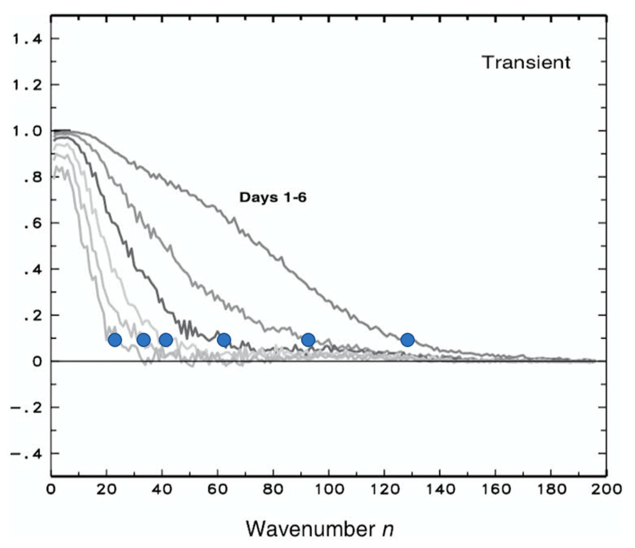
2.2. Loss of Skill as a Function of the Scale

So far, we have discussed the total error and skill in forecasts. It has been long recognized, however, that forecast error and skill, hence predictability, is a strong function of scale. Roads [29,30], for example, found that the error in time mean forecasts, which is dominated by larger spatial scales, is lower than in instantaneous forecasts. Other relevant studies of the relationship between scale and skill include Dalcher and Kalnay [15], Clark et al. [31], Buizza and Leutbecher [32], and Toth and Buizza [33]. Some conclusions from some of these studies are well summarized by Boer [34] and reproduced here as Figure 1.

Boer [34] studied the loss of skill, or error growth, in 500 hPa height forecasts, as a function of scale and lead time. As demonstrated earlier by other studies (e.g., [15]), he showed that the loss of skill occurs rapidly at high wavenumbers, while lower wavenumbers are affected at a slower rate. As an example, the skill at wavenumber 60 is almost completely lost in 3 days, while the skill at wavenumber 20 is retained for 6 days (Figure 1). The faster loss of skill at high wave numbers is associated with a quick saturation of error on the fine scales, while the saturation for larger waves with lower wavenumbers occurs over a longer period.

The faster/slower saturation of error at smaller/larger scales is a fundamental property and is related, somewhat trivially, to the organization of processes in the atmosphere. The turbulent nature of atmospheric dynamics has been linked to self-similarity, where similar behavior occurs on a wide range of scales. In such an environment, and at a given rate of incoming and outgoing energy flow (e.g., solar radiation), “energizing” and completing processes on smaller/larger scales simply takes a shorter/longer time [25,35]. In the next subsection, we present the results of an investigation of the lead time at which the skill drops to near zero as a function of wavelength.

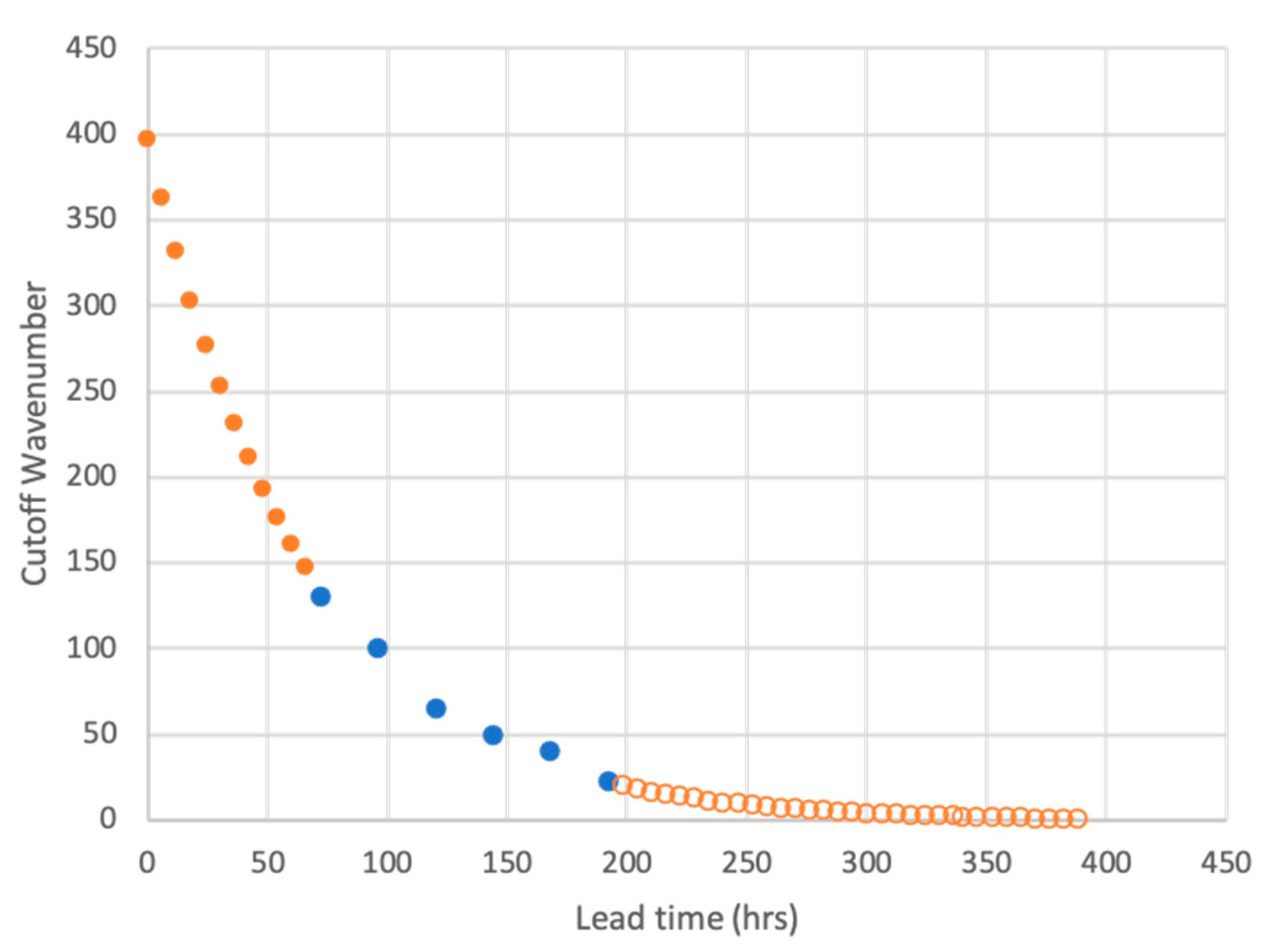
2.3. Quantitative Estimate

In our quest to understand how forecast skill is lost, we first investigated the lead time at which forecast features of different scales lose most of their skill. For this, we return to Figure 1, where for each lead time, we marked the wavenumber whose skill drops to a marginal level of 0.1 PAC (i.e., the “cutoff wavenumber”, blue dots in Figure 1). Waves larger than any particular cutoff wavenumber are at least partially predictable, while the forecast anomaly of smaller waves (with higher wavenumbers) explains less than 1% variance in the anomaly of the verifying analysis. These smaller-scale waves thus have only negligible or no skill (i.e., unpredictable scales).

The blue dots from Figure 1 are transposed into the cutoff wavenumber vs. lead time coordinate space of Figure 2. Boer’s [34] results reproduced in Figure 1 reflect the skill of NWP systems about 20 years ago. Before we replotted these results in Figure 2, we adjusted the lead time of forecasts to reflect today’s NWP skill. Considering that NWP systems gain approximately 1 day of skill per decade [23], 2 days were added to the lead time of all blue points in Figure 1 before they were replotted as blue dots in Figure 2. Lead times of 1–6 days in Figure 1 thus became 3–8 days in Figure 2.

A casual inspection of the scales with negligible skill as a function of lead time (blue dots in Figure 2) suggested an exponential relationship between the lead time and cutoff wavenumber. This observation was confirmed experimentally: an exponential curve (orange circles) offered the best fit to the observed data points in Figure 2, which were acceptable at the 99% statistical confidence level. Our results were corroborated by a study of simulated analysis and forecast error data by Privé and Errico [36]. Apart from the largest error magnitudes approaching the climatic variance, power spectrum curves for forecast error displayed on a logarithmic scale in their Figure 1 are close to being equally spaced as a function of lead time, as measured on a linear scale, indicating an exponential progression of error magnitude. This corresponded with the exponential placement of points in Figure 2 of the present study.

Assuming again self-similarity in turbulent atmospheric perturbations over a wide, so-called “inertial” range (from at least hundreds of kilometers down to possibly centimeter scales [24,25]), the exponential relationship found in Figure 2 may indeed be theoretically founded. Based on this analysis, the best fit exponential curve was used to extrapolate Boer’s [34] cutoff data in the 0–20-day lead time range. The orange dots on the left side of Figure 2 represent an extrapolation of the empirically found exponential relationship to smaller magnitudes down to the estimated error in current initial conditions. At the initial time, the cutoff wavenumber was around 400, suggesting that today’s global NWP analysis fields cannot capture features finer than 50–100 km in scale. In other words, the nominal grid resolution of today’s global circulation models is around 10 km. The description of any feature in a model requires at least 3–5 grid points, which indicates that features with a scale below about 50 km, even if observed well, could not be realistically represented in an analysis.

Though without observational data or further analysis, an extrapolation to larger scales may theoretically be less defendable, the open circles on the right side of Figure 2 indicate such extrapolated values as a zeroth order estimate of the cutoff wavenumbers. Without any related constraint, the best fit exponential curve in Figure 2 is seen to asymptotically tend toward a zero wavenumber (representing the largest, global scale) at very long lead times, suggesting that the right-hand extrapolation (open circles in Figure 2) may, after all, offer an acceptable estimate. Having estimated the lead time at which skill for different scales is lost, high-frequency variability below the cutoff wavenumber shown in Figure 2, which was thought to be noise, was removed from forecasts at all lead times before any further analyses were performed (Section 3.2). Our attention now turns to the processes through which the loss of forecast skill occurs.

3. Approach

As seen from Figure 1, at large scales, forecasts begin with a high PAC level, which is indicative of high forecast information. In the next sections, we attempt to describe some processes through which, in a matter of days in lead time, near-perfect forecasts become almost useless, i.e., devoid of skill. Is it the structure and amplitude of forecast features that deviate from observations first? Or is the skill lost primarily due to the misplacement of forecast features that eventually become out of phase from the observed weather?

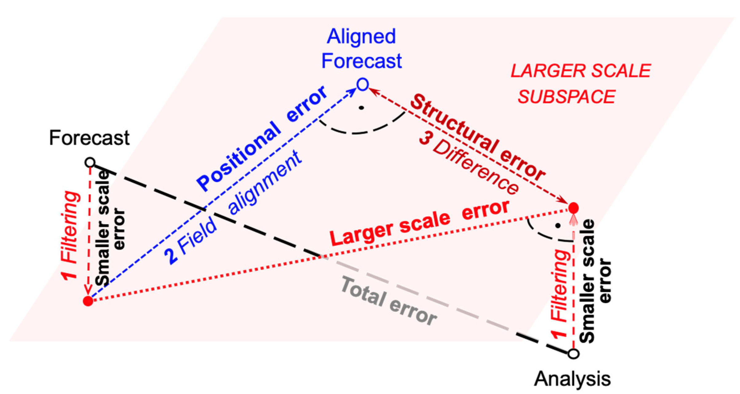
3.1. The Concept of Error Decomposition

Due to the chaotic nature of the atmosphere, weather forecasts, even with ever-improving numerical models, diverge from reality. Synoptic experience indicates that the atmosphere comprises spatiotemporally coherent structures, such as low-pressure systems and fronts, which with increasing lead time are progressively displaced and distorted in numerical forecasts [37,38]. Hence, weather forecasts are affected by both positional and structural (or amplitude) errors. This has long been recognized by practicing forecasters. Tropical cyclones (TC), for example, have been considered coherent features that move through space. Tracking and intensity errors were introduced to assess the performance of TC [39], and later, extratropical cyclones [40], and then other forecast features (e.g., [41,42]).

In recent decades, various objective methods for the diagnosis of positional and structural components of entire 2D forecast error fields were developed; for a brief overview, see Jankov et al. [43]. Nonetheless, most routine verification or statistical post-processing methods implicitly assume that forecasts have no positional error and assess only the magnitude of the total error [44]. In the present study, through the decomposition of the forecast error and ensemble spread, we evaluated whether forecast skill is lost primarily due to the displacement or the distortion of weather features.

3.2. Experimental Data

The loss of skill is studied with a 500 hPa height ensemble forecast (initialized at 00Z) and verifying analysis data from the National Centers for Environmental Prediction (NCEP) Global Ensemble Forecasting System (GEFS) and the Global Forecast System (GFS, [45]).

The analysis was performed globally on a 13 km grid for the 1 January–31 March 2020 experimental period. For computational economy, only 48 h, 120 h, 168 h, 240 h, 360 h, and 384 h lead time forecasts were studied. Before spatial filtering as described next, both the forecast and analysis data were expressed in terms of their anomaly from the 20-year reanalysis climatic mean [46].

3.3. Methodology

Finer-scale error. In the upcoming analysis, the total forecast error was partitioned into three orthogonal components. The first component was associated with forecast features that lost most of their skill, i.e., those characterized by wavenumbers higher than those indicated by the orange discs in Figure 2. The variance at these smaller, unpredictable scales were removed from both the forecast and the verifying analysis fields using a low-pass Butterworth filter [47] with lead-time-dependent cutoff values from Figure 2 (see Step 1 in Figure 3). It is worthwhile mentioning that, for our analysis, the ensemble mean forecasts were not filtered any further, as the mean of a reasonably sized ensemble offers a natural filter of unpredictable scales [48,49], Having no forecast skill on these scales, the smaller-scale structures from the two fields, by definition, are orthogonal; therefore, the sum of their variances defined the error at the unpredictable scales (i.e., the smaller-scale component of the total error). We called the remaining part of the total variance the larger-scale component.

Positional and structural error. For the decomposition of the larger-scale error field into the second, positional, and third structural components, we used a modified version of Jankov et al.’s [43] methodology. In particular, using the field alignment (FA) method of Ravela et al. [50], the larger-scale forecast field was aligned with the larger-scale (filtered) verifying analysis field using a variationally determined smooth vector field so that its difference from the larger-scale analysis field was minimized. The positional error was defined as the variance (or rms) difference between the original and aligned larger-scale (filtered) forecast fields (see Step 2 in Figure 3), while the structural error was the variance (or rms) difference between the aligned larger-scale forecast and the larger-scale verifying analysis fields (see Step 3 in Figure 3). Replacing the verifying analysis with the mean of the ensemble in the above algorithm yielded an orthogonal decomposition of the variance of ensemble members around their mean. For clarity, the definition of the different error and ensemble variance components used in this study are listed in

Table 1. Differences used in the definition of the forecast error (in this example, error in the ensemble mean forecast, which was not filtered any further) and ensemble variance components.

Variance Type	Error Variance in the Mean	Ensemble Variance around the Mean
Total	Difference between the original ensemble mean and the analysis	Difference between the original/unmodified ensemble members and the original ensemble mean
Larger-scale	Difference between the filtered ensemble mean and the filtered analysis	Difference between the filtered ensemble members and the original ensemble mean
Smaller-scale (unpredictable)	Difference between the original and filtered verifying analysis	Difference between original and filtered ensemble members
Positional	Difference between the filtered ensemble mean and the aligned filtered ensemble mean	Difference between the filtered ensemble members and the aligned filtered ensemble members
Structural	Difference between the aligned filtered ensemble mean and the filtered analysis	Difference between the aligned ensemble members and the original ensemble mean

.

As a demonstration of the methodology, Figure 4 shows the 500 hPa geopotential height original (Figure 4a) and filtered analysis (Figure 4b) anomalies; the corresponding 10-day lead time ensemble mean forecast anomaly, overlaid with the displacement vector field (Figure 4c); and the ensemble mean anomaly aligned with the filtered analysis (Figure 4d) valid on 11 January 2000 at 0000 UTC. The most pronounced larger-scale features on the unfiltered analysis (Figure 4a) were two positive 500 mb geopotential height anomalies: one south of Alaska and the other along the east coast of NA. A sizable negative geopotential height anomaly comprising a series of smaller-scale lows located over Southern Greenland and extending into the central Atlantic Ocean was also notable. The application of the low-pass filter only had a moderate effect on the two large-scale highs; however, smaller-scale features in the Southern Greenland—Atlantic low area and elsewhere (see, e.g., lows over the Aleutian Islands and the west coast of NA, Figure 4b) were notably more affected.

Moving the ensemble mean forecast anomaly along with the blue displacement vectors in Figure 4c created a forecast that was aligned with the corresponding filtered observational analysis anomaly (Figure 4d). The displacement vectors tended to be large in areas where anomaly features in the filtered forecast and filtered analysis fields were out of phase. Examples included a low anomaly that the ensemble mean placed SE of the southeastern portion of the analyzed Southern Greenland—Atlantic area, which needed to be moved NW, and a high-pressure forecast feature over the area of the observed weak low anomaly over the Aleutian Islands, which was moved over the large high pressure analyzed anomaly to the west.

In contrast, in areas where the forecast and analysis anomalies were well aligned and in good agreement, the displacement vectors tended to diminish (see, e.g., the center of the south of Alaska and East Coast of NA highs, Figure 4c) compared with the ensemble mean anomaly due to the orthogonal decomposition of the ensemble mean (anomaly) error into its positional and structural components. Given this was a smooth vector field, only part of the ensemble mean forecast anomaly could be aligned with the filtered verifying analysis, and thus, the magnitude of anomalies in the aligned ensemble mean was notably reduced.

4. Decomposition of Error and Perturbation Variances

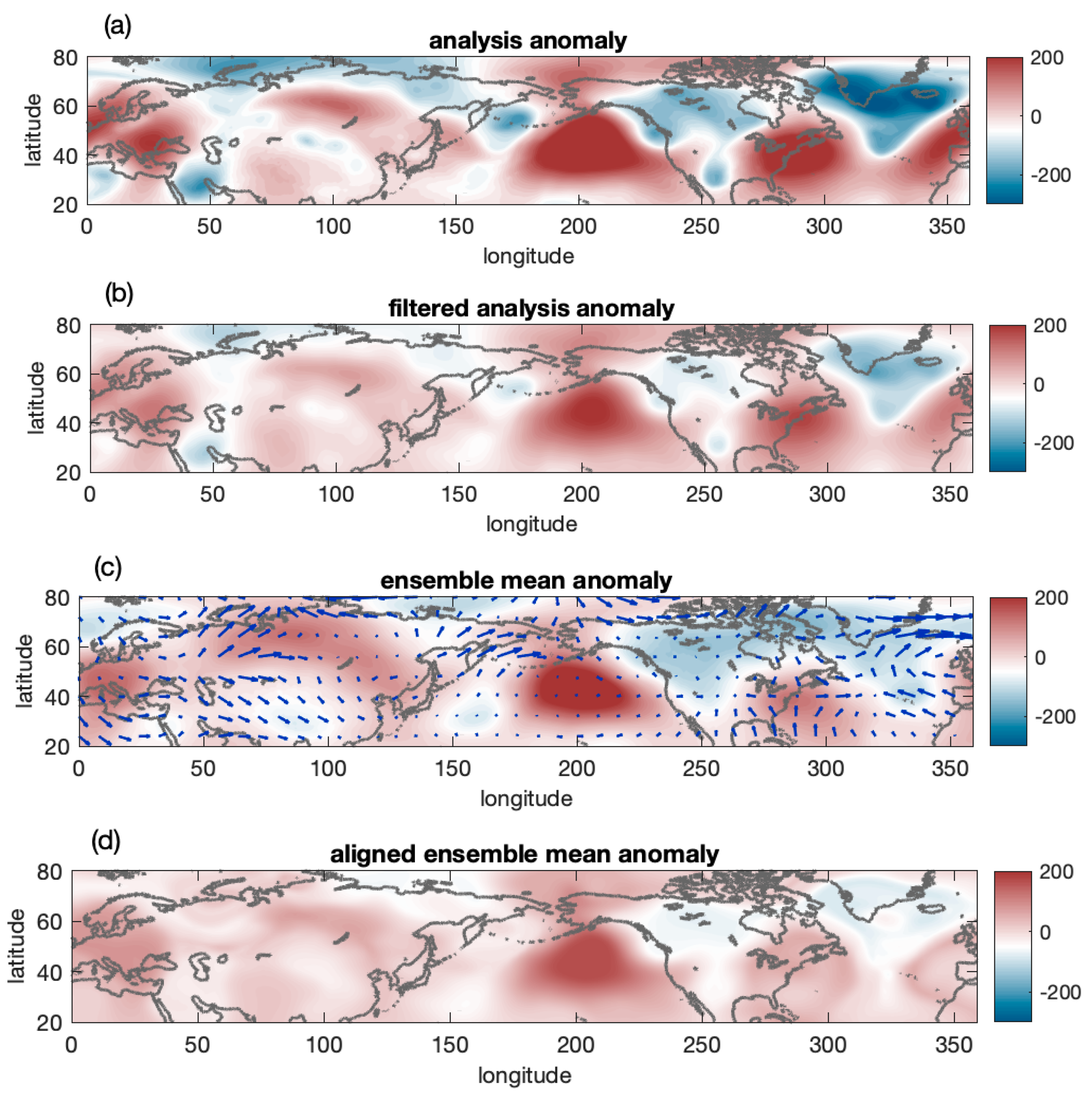
4.1. An Example

The decomposition of error variance in and perturbation variance around the mean of the 20-member GEFS ensemble is demonstrated in Figure 5 and Figure 6, respectively, for the case shown in Figure 4. Not surprisingly, at 10 days lead time, the forecast of the three highlighted and many of the other features had only limited skill (cf. Figure 4b,c). What is behind the failure of the forecast? Positional or structural problems in the forecast? Or are the scales of some features already finer than what is predictable at a 10-day lead time?

A quick look at Figure 5 revealed that in this case, the positional (panel b) and structural components of the error (panel c) were comparable in size, while the smaller-scale error variance (panel d) was lesser in magnitude. This was suggestive of a situation where at a larger scale, partially predictable variance still dominated the forecast. Perturbation variance, on the other hand, was concentrated in the smaller-scale component, with less variance in the positional, and virtually no variance in the structural larger-scale components (Figure 6).

More specifically, related to the high south of Alaska, at higher latitudes, we saw a clear sign of positional error in the form of a positive–negative dipole over the Aleutian Islands. This was indicative of a westward shift in the forecast compared with the analysis (cf. Figure 4b,c). The application of either the displacement vectors or the inverse of the positional error field to the ensemble mean anomaly moved the forecast high eastward, remedying part of the problem. On the other hand, the structural or smaller-scale error variance was small in this area. The large positional and small structural error was consistent with the subjective observation that the forecast high had an approximately correct amplitude, but was placed at the wrong location (cf. Figure 4c,d).

The high over the east coast of NA, on the other hand, was dominated by a structural error in the form of a large monopole centered over it. The positional error indicated a small displacement of the forecast high to the SW, while a smaller-scale error was negligible. The large structural error reflected the subjective observation that the high-pressure anomaly was well positioned but not strong enough in the forecast (cf. Figure 4b,c). The situation was similar for the Southern Greenland low: structural error dominated, with small and negligible positional and smaller-scale components, respectively. This was consistent with the forecast low, except for its SE extension, with it being positioned (Figure 4d) close to its analyzed location but with less intensity.

As noted above, in this case, smaller-scale perturbation variance dominated the ensemble spread. Interestingly, all three areas with high smaller-scale variance were associated with forecasts that were fully out of phase (hence, they lost all skill) compared with the analysis (cf. Figure 4b,c) of the mid-Atlantic, an area from the northern British Isles to SE of Scandinavia, and the Eastern Pacific (note the large difference in the orientation of the gradient in the forecast and analyzed fields for the latter feature). To assess how typical error and perturbation behavior observed in this case was, next we looked at longer-term statistics. We found that a statistical analysis may also help with the interpretation of results for individual cases.

4.2. Statistics

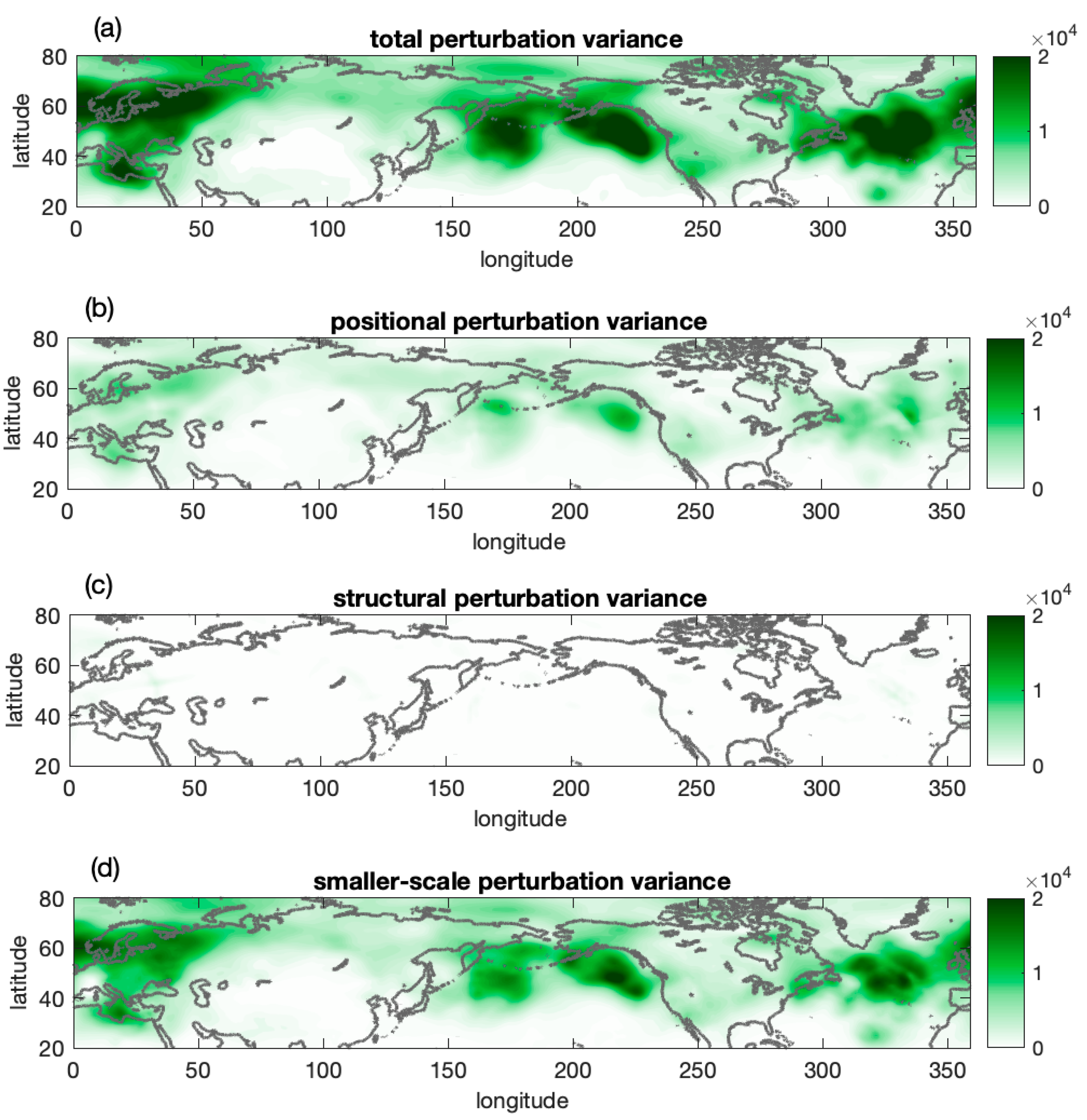
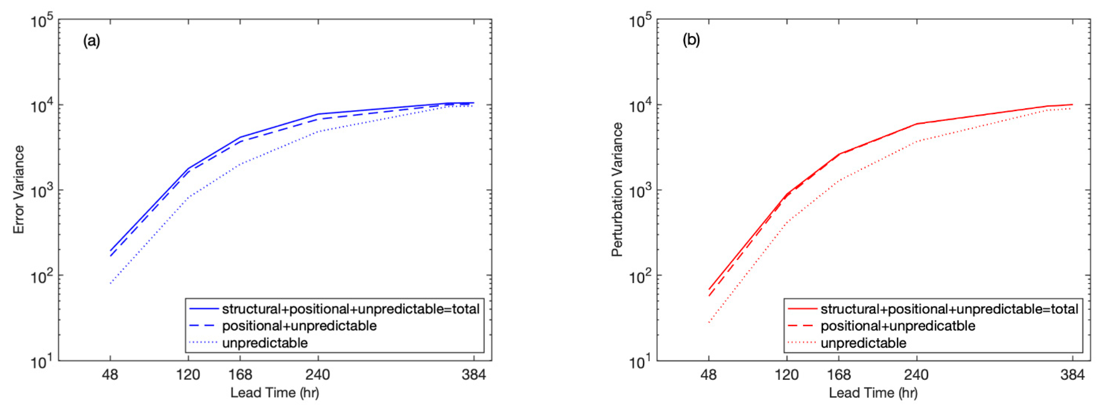
4.2.1. Total and Scale Dependent Variances

Figure 7a,b show the unpredictable smaller-scale (dotted curves at the bottom) and vertically stacked larger-scale positional (between dotted and dashed lines) and larger-scale structural (between dashed and solid lines) error variances in, and perturbation variance around, the ensemble mean Northern Hemisphere extratropical (20° N–80° N) 500 hPa height forecast, respectively. First, we noted that the presumed initial linear growth of the total error and perturbation variances (top lines in panels (a) and (b), respectively), as expected, was tempered after day 5, as the variances assumed a slower growth, followed by nonlinear saturation (solid lines in Figure 7). This was consistent with the findings of Pena and Toth [14], Feng et al. [12], and Zhou et al. [51]. For a short lead time, the sum of the larger-scale positional and structural variances exceeded that of the unpredictable smaller-scale variances and grew similarly fast. Note that the mean of an ensemble removed a large part of the unpredictable variance present in a single, unperturbed forecast. Hence, the smaller-scale error variance of completely unpredictable scales was significantly (by close to a factor of 2) reduced.

Beyond a 10-day lead time, however, unpredictable smaller-scale variances became dominant in the total error and perturbation variances, as by day 16, almost all the skill was exhausted.

Another observation from Figure 7, which is also well documented elsewhere, is that perturbation variance around the ensemble mean was somewhat deficient compared with the error variance in it [1,52,53]. Feng et al. [13] argued that the deficiency at short lead times may only be an appearance due to a bias in error variance estimates due to a correlation between the error pattern in the forecast and verifying analysis fields. Despite their lower value, as seen further below, ensemble variance can be a valuable tool in untangling initial-value- vs. model-related forecast errors. To make comparisons between the error and ensemble variances more straightforward, before they were replotted in Figure 8, variances from Figure 7 were standardized at each lead time separately using the total error/ensemble variance.

Next, we noted that the ratio of the variances associated with unpredictable smaller, and partially predictable larger scales (i.e., the sum of positional and structural), as demarcated by the dotted lines in Figure 8, were similar for the errors (blue) and perturbations (red). This was by design, as the smaller-scale variance was filtered out both for the error and ensemble variance calculations using the same Butterworth filter (Section 3.2). The partition of larger-scale variance into positional and structural components, however, was quite different for the error and ensemble perturbations.

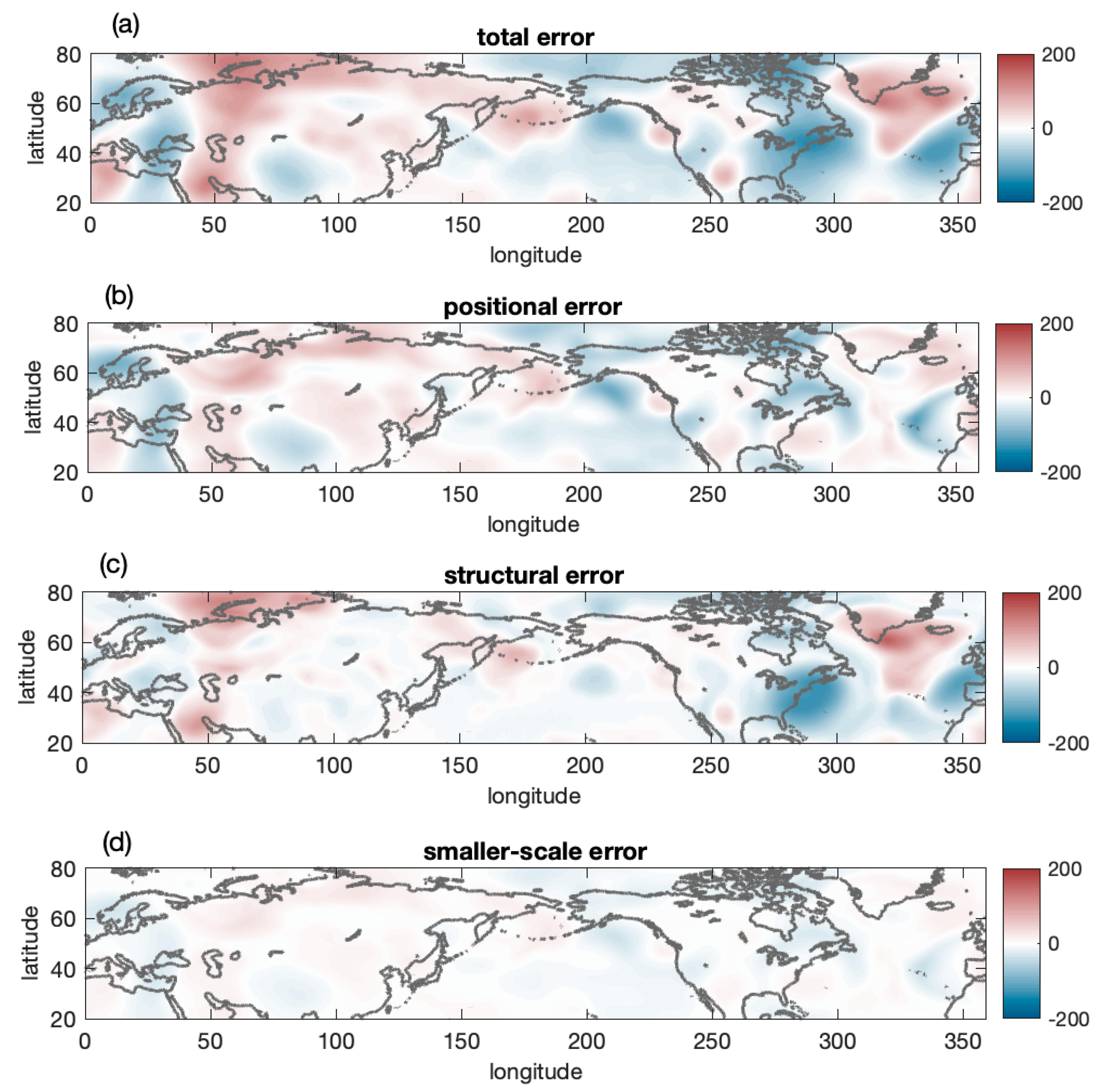
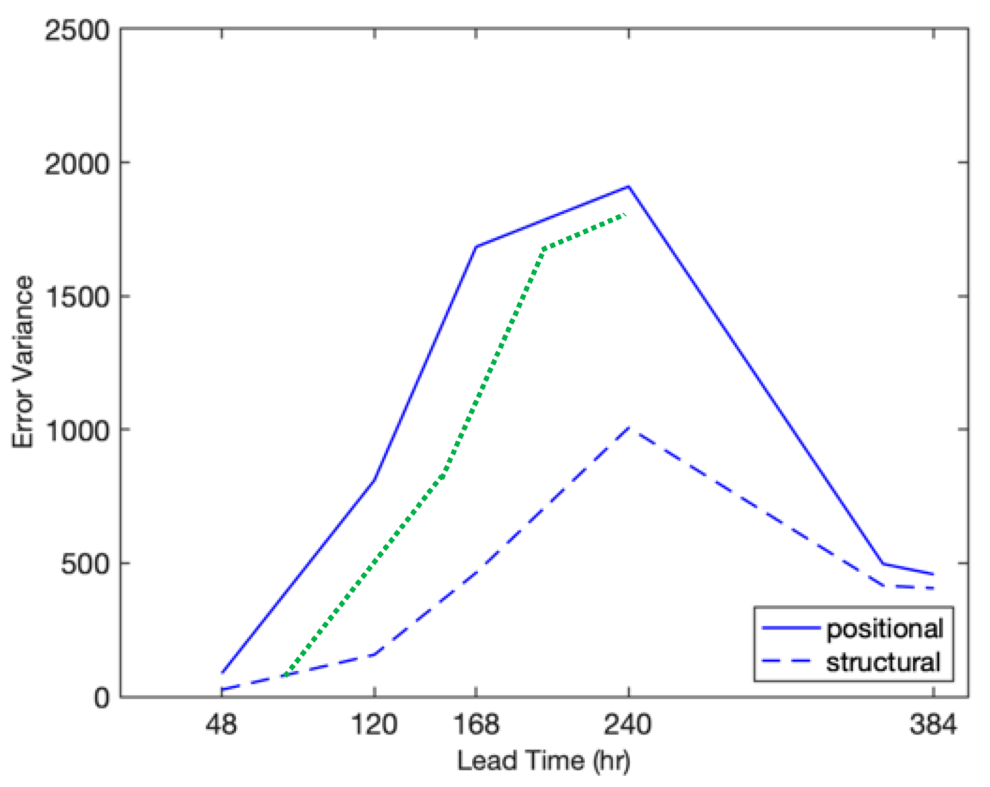
4.2.2. Positional and Structural Variances

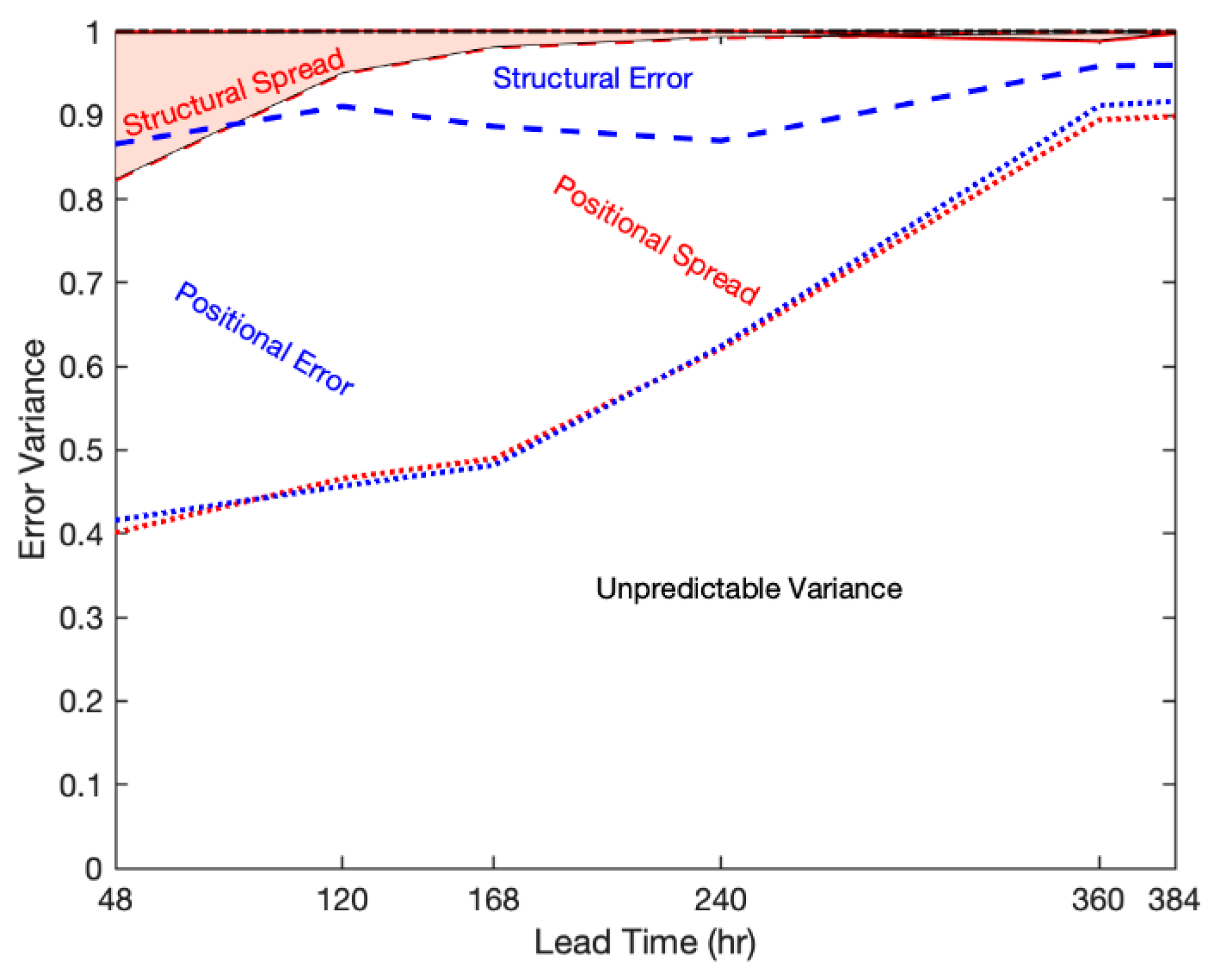
First, we noted that at most lead times, the positional variance dominated the structural variance for both the errors and perturbations. This was consistent with Jankov et al.’s [26] short-range error analysis. The structural component on day 2 was about 15% of the total, and 25% of the larger-scale variance, both for the errors and perturbations (Figure 8). The structural perturbation variance rapidly declined early on, having virtually diminished completely by day 10 (Figure 7). In contrast, the portion of the structural error remained steady (which meant continued growth in an absolute sense) through to day 10, only after which it dropped. After that, as most skill disappeared, the structural error became comparable in magnitude with the positional error. A possible interpretation of these results in terms of the initial-value- vs. model-induced forecast error followed.

5. Interpretation

As discussed in Section 2, initial errors are amplified exponentially. Meanwhile, past studies approximated the evolution of model-induced forecast errors differently. Leith [18,54] suggested, and using extratropical forecast data, Dalcher and Kalnay [15] tested the idea that during model integrations, imperfect models induce the same amount of error variance at each time step, leading to initially linear growth in the model-related forecast error. On the other hand, Peña and Toth [14] found that in the tropics, model-related error variance can be well described with a saturating exponential curve. Interestingly, using more recent NWP forecasts, Peña and Toth [14], Feng et al. [12,13], and Zhou and Toth [23] could describe the total error in the sub- and extratropics with a single exponential curve without the introduction of an extra term for model-induced error.

An important consideration for the interpretation of positional and structural error results above is that in an ensemble like NCEP’s GEFS, where each member is generated with the same numerical model, the growth of the perturbation variance among members is driven exclusively by the chaotic amplification of differences in the initial condition. These member-to-member differences, unlike forecast error, are not influenced by model error. Perturbation variance may be affected by model error only over a short, transitional period, over which the influence of the observed initial condition, somewhat inconsistent with model dynamics, dies out. In other words, when a forecast is initialized with observed initial conditions, as is done in current NWP practice, a transitionary behavior ensues, which at shorter lead times may invoke structural differences between ensemble members. Therefore, larger-scale structural error at later lead times was the first clear indication in our study of the presence and the level of model-related error in weather forecasts.

Another consideration followed from the observation that at and beyond 5 days lead time, structural perturbation variance diminished to about 1% of the total perturbation variance. As the GEFS ensemble has no model-induced variability, the lack of structural perturbation variance beyond short lead times was an indication that initial-value-related uncertainty, which is unaffected by the model error, mostly manifested as a displacement and not as a distortion of forecast circulation systems.

A possible explanation for the initial condition error primarily manifesting as positional as opposed to a structural forecast error invoked the notion that atmospheric dynamics involved the cascading growth and propagation of energy through waves of progressively larger scales. In the early, linear phase of evolution, waves in each band develop mostly independently, without much influence from other waves [55]. Slightly different initial conditions can therefore manifest only in variations in the position (i.e., the phase), and not the amplitude (or structure) of waves. As saturation sets in, waves lose all their skill and become unpredictable, with the associated error being classified in this study as “smaller-scale”. In contrast, structural error in the medium and extended ranges hovered around 10% of the total error variance (Figure 8), which we interpreted as the manifestation of a moderate level of model-induced error.

For the discussion below, the positional and structural error variance components from Figure 7 were reproduced on a linear scale as the blue solid and dashed curves in Figure 9. Both error components had an exponentially growing pattern, at least until 7 days lead time. Considering the literature cited above [18,24], this suggested that both the positional and structural errors may be initial value related. As noted above, however, structural ensemble perturbation variance diminished after a few days and constituted only about 1% of the total perturbation variance (Figure 8). The virtual lack of structural ensemble perturbation variance was thus a clear indication that structural error variance must originate from model imperfections. Even though the model error may be dominated by exponentially growing structural variance, there were other types of model-induced forecast problems, including systematic error in the speed of atmospheric waves [56]. Note also that the systematic model error not correctable by the observing system remained undetected.

How can the exponential growth of model-induced error be reconciled with earlier findings of linear or saturating exponential growth?

We hypothesized that model error primarily manifests as modes of natural variability (e.g., the Madden–Julian oscillation (MJO) circulation) that are missed by numerical models. Following Peña and Toth [14], we also assumed that if a mode is completely missed by a model, through a transitional behavior, analyzed features of such modes quickly disappear from model integrations. This results in a saturating exponential growth of error. This behavior is readily observed in the tropics (see the dashed curve of Figure 8 in Peña and Toth [14]), as lower or moderate resolution models with conventional convective parameterization schemes cannot resolve significant parts of the large-scale tropical circulation (e.g., the MJO [57]).

We further speculated that when a mode of natural variability is only partially missed, or mostly but not completely captured, such as the extratropical circulation considered by models of the 1980s or today, respectively, the initial growth in the model-induced error may be tempered. Such behavior can then be approximated by linear or exponential growth, as seen, e.g., in Figure 6 of Dalcher and Kalnay [15], and via the green dashed line in Figure 9 of the present study, respectively. According to this hypothesis, a complete/partial/limited lack of dynamics related to missed natural modes of variability may lead to a gradual shift in the initial behavior of the model-related error, from the fastest (saturating exponential in the tropics) and intermediate (linear, extratropics in models of the past) to the least rapid growth (exponential, extratropics in today’s models). Future studies may confirm and explain in more detail such a pattern of model-induced error behavior.

We would be amiss not to mention a notable difference between the growth rates of positional and structural error in Figure 9. As discussed earlier, the positional error is significantly larger than the structural error. Since the exponential growth rate per unit time strongly depends on error amplitudes, for a more informed comparison, the growth rates for the two error components were compared over periods that started with the same initial variance. For this, the evolution of the positional error was replotted in a horizontally translated position (green dotted line), starting from a value on the structural error variance curve. Remarkably, the growth of the positional error was significantly higher than that of the structural error. As for the factor of two difference in growth rates in Figure 9, when a verifying analysis with a natural feature is compared with a forecast that systematically misses such features, the related forecast error will be half of that compared with a model that captures natural variability related to the feature considered. Therefore, the factor of two difference in error growth rates observed in Figure 9 was consistent with the structural error being model-induced. This was a second observation suggesting that structural error may be model induced, with causes and processes likely distinct from the positional error.

As pointed out above, Peña and Toth [14], Feng et al. [12,13], and Zhou and Toth [23] found that the total extra- and sub-tropical short-range forecast error variance can be well explained with a single exponential curve. These and even earlier studies (e.g., [21,22]) tentatively concluded that NWP models may be near perfect at the scales they resolve, and may have only negligible model-induced error components. We note, however, that in some cases and over limited ranges, the sum of two exponentials (such as the solid and dashed curves in Figure 9) may be well approximated with a single exponential curve. Hence, the exponential-looking total error curves in the earlier studies may in fact hide a smaller portion of slower, but still exponentially growing model-related error, which would be consistent with the 10% structural error, interpreted as a model-induced error, that was found up until 10 days lead time in the current study.

In summary, we interpreted the orthogonal positional and structural error components as the primary manifestation of initial-value- and model-related forecast error, respectively. The large positional error associated with the south of Alaska high shown in Figure 4 and Figure 5 may be a good example of a case where the forecast error primarily originated from inaccurate initial conditions. Meanwhile, the high- and low-pressure systems over the east coast of NA and South (of) Greenland, respectively, both of which were simulated by the model, but with too low intensity, may be good examples of the partial missing of natural modes of variability by a model.

Past diagnostics of model error include systematic forecast error and the parametric description of temporal error behavior (e.g., [14]). While some model errors may manifest as case-dependent systematic errors (e.g., when highs and lows such as those highlighted above may not develop deep enough), such errors will not necessarily show up in the overall time mean systematic error. At the same time, the parameterized temporal description method cannot geographically localize the model error. The phenomenological alignment–amplitude decomposition of the larger-scale error into orthogonal positional and structural components introduced in this study, on the other hand, would readily identify and geographically localize otherwise elusive model-related errors. This or similar methods may offer a potential new tool for future model development efforts.

6. Conclusions

Despite numerous related studies, ambiguity still abounds as to the role of model-induced errors in numerical forecasting. In studying how forecast performance degrades in the extratropics, the “cut-off” wavenumber/scale beyond which forecast variability has no skill was found to drop/grow exponentially as a function of the lead time (Figure 2). Using this cut-off wavenumber, the forecast error variance was decomposed into scales that partially (larger-scale variability) and completely (smaller-scale variability) lost skill. An extrapolation of the exponential relationship to the initial time indicated that at scales finer than 50–100 km, global analysis fields were unrelated to reality. At short lead times where the skill was still high, the total error variance was dominated by the error at the partially predictable scales, while beyond 7 days, this domination occurred at completely unpredictable scales.

An additional orthogonal decomposition of the error variance over the partially predictable (and lead-time dependent) larger scales showed that over the first seven forecast days, both positional and structural error components evolved approximately exponentially. The positional error, however, grew twice as fast. The positional error was exemplified with dipoles, while the structural error was exemplified with monopoles, suggesting that different processes may be responsible for each type of error. The positional error was found to dominate the larger-scale error till day 10, with structural error hovering around 10% of the total error variance. In contrast, a similar decomposition of ensemble perturbations revealed that structural perturbation variance was virtually nonexistent after a few days of lead time. Given that all members of the NCEP ensemble were generated with the same procedure, we concluded that (1) initial-value-related error manifested primarily as the positional error, while (2) model-induced error mostly manifested as the structural error.

The structural error was about 10% of the total error variance. The mean of an ensemble had a much-reduced error compared with an unperturbed forecast. The fact that 10% of the total error in the ensemble mean was structural suggested that, in general, less than 10% of NWP forecast error variance may be caused by model deficiencies. These results offer qualification of earlier subjective and objective assessments of the role of model-induced forecast deficiencies. The orthogonal decomposition of total error variance introduced in this study thus potentially offered a new approach to the statistical assessment and geographical localization of model-induced error, with possible applications in model development.

References

1. Buizza, R.; Houtekamer, P.L.; Pellerin, G.; Toth, Z.; Zhu, Y.; Wei, M. A comparison of the ECMWF, MSC, and NCEP global ensemble prediction systems. Mon. Weather Rev. 2005, 133, 1076–1097. [Google Scholar] [CrossRef]
2. Duan, W.; Liu, X.; Zhu, K.; Mu, M. Exploring the initial errors that cause a significant “spring predictability barrier” for El Niño events. J. Geophys. Res. Ocean. 2009, 114, C04022. [Google Scholar] [CrossRef]
3. Grams, C.M.; Magnusson, L.; Madonna, E. An atmospheric dynamics perspective on the amplification and propagation of forecast error in numerical weather prediction models: A case study. Q. J. R. Meteorol. Soc. 2018, 144, 2577–2591. [Google Scholar] [CrossRef]
4. Houtekamer, P.L.; Mitchell, H.L. Data assimilation using an ensemble Kalman filter technique. Mon. Weather Rev. 1998, 126, 796–811. [Google Scholar] [CrossRef]
5. Molteni, F.; Buizza, R.; Palmer, T.N.; Petroliagis, T. The ECMWF ensemble prediction system: Methodology and validation. Q. J. R. Meteorol. Soc. 1996, 122, 73–119. [Google Scholar] [CrossRef]
6. Toth, Z.; Kalnay, E. Ensemble forecasting at NCEP and the breeding method. Mon. Weather Rev. 1997, 125, 3297–3319. [Google Scholar] [CrossRef]
7. Buizza, R.; Milleer, M.; Palmer, T.N. Stochastic representation of model uncertainties in the ECMWF ensemble prediction system. Q. J. R. Meteorol. Soc. 1999, 125, 2887–2908. [Google Scholar] [CrossRef]
8. Palmer, T.N.; Buizza, R.; Doblas-Reyes, F.; Jung, T.; Leutbecher, M.; Shutts, G.J.; Steinheimer, M.; Weisheimer, A. Stochastic Parametrization and Model Uncertainty; European Centre for Medium-Range Weather Forecasts: Reading, UK, 2009. [Google Scholar]
9. Shutts, G. A kinetic energy backscatter algorithm for use in ensemble prediction systems. Q. J. R. Meteorol. Soc. 2005, 131, 3079–3102. [Google Scholar] [CrossRef]
10. Craig, G.; Forbes, R.M.; Abdalla, S.; Balsamo, G.; Bechtold, P.; Berner, J.; Buizza, R.; Pallares, A.C.; De Meutter, P.; Düben, P.D.; et al. What Are the Sources of Model Error and How Can We Improve the Physical Basis of Model Uncertainty Representation? Available online: https://www.researchgate.net/publication/311283383_What_are_the_sources_of_model_error_and_how_can_we_improve_the_physical_basis_of_model_uncertainty_representation (accessed on 12 August 2022).
11. Nicolis, C.; Perdigao, R.A.; Vannitsem, S. Dynamics of prediction errors under the combined effect of initial condition and model errors. J. Atmos. Sci. 2009, 66, 766–778. [Google Scholar] [CrossRef]
12. Feng, J.; Toth, Z.; Peña, M. Spatially extended estimates of analysis and short-range forecast error variances. Tellus A Dyn. Meteorol. Oceanogr. 2017, 69, 1325301. [Google Scholar] [CrossRef] [Green Version]
13. Feng, J.; Toth, Z.; Peña, M.; Zhang, J. Partition of analysis and forecast error variance into growing and decaying components. Q. J. R. Meteorol. Soc. 2020, 146, 1302–1321. [Google Scholar] [CrossRef]
14. Peña, M.; Toth, Z. Estimation of analysis and forecast error variances. Tellus A Dyn. Meteorol. Oceanogr. 2014, 66, 21767. [Google Scholar] [CrossRef]
15. Dalcher, A.; Kalnay, E. Error growth and predictability in operational ECMWF forecasts. Tellus A 1987, 39, 474–491. [Google Scholar] [CrossRef]
16. Hopson, T.M. Assessing the ensemble spread–error relationship. Mon. Weather Rev. 2014, 142, 1125–1142. [Google Scholar] [CrossRef]
17. Whitaker, J.S.; Loughe, A.F. The relationship between ensemble spread and ensemble mean skill. Mon. Weather Rev. 1998, 126, 3292–3302. [Google Scholar] [CrossRef]
18. Lorenz, E.N. Deterministic nonperiodic flow. J. Atmos. Sci. 1963, 20, 130–141. [Google Scholar] [CrossRef]
19. Yuan, H.; Toth, Z.; Peña, M.; Kalnay, E. Overview of weather and climate systems. In Handbook of Hydrometeorological Ensemble Forecasting; Springer: Berlin/Heidelberg, Germany, 2019; pp. 35–65. [Google Scholar]
20. Du, J.; Berner, J.; Buizza, R.; Charron, M.; Houtekamer, P.L.; Hou, D.; Jankov, I.; Mu, M.; Wang, X.; Wei, M.; et al. Ensemble Methods for Meteorological Predictions; National Centers for Environmental Prediction (NCEP): College Park, MD, USA, 2018. [Google Scholar]
21. Leith, C.E. Theoretical skill of Monte Carlo forecasts. Mon. Weather Rev. 1974, 102, 409–418. [Google Scholar] [CrossRef]
22. Kleeman, R. Information theory and dynamical system predictability. Entropy 2011, 13, 612–649. [Google Scholar] [CrossRef]
23. Zhou, F.; Toth, Z. On the prospects for improved tropical cyclone track forecasts. Bull. Am. Meteorol. Soc. 2020, 101, E2058–E2077. [Google Scholar] [CrossRef]
24. Lorenz, E.N. Irregularity: A fundamental property of the atmosphere. Tellus A 1984, 36, 98–110. [Google Scholar] [CrossRef]
25. Lorenz, E.N. The predictability of a flow which possesses many scales of motion. Tellus 1969, 21, 289–307. [Google Scholar] [CrossRef]
26. Weisstein, E.W. CRC Concise Encyclopedia of Mathematics; Chapman and Hall: London, UK; CRC: Boca Raton, FL, USA, 2002. [Google Scholar]
27. Murphy, A.H.; Epstein, E.S. Skill scores and correlation coefficients in model verification. Mon. Weather Rev. 1989, 117, 572–582. [Google Scholar] [CrossRef]
28. Kim, H.; Kim, H.; Son, S.W. The influence of MJO initial condition on the extratropical prediction skills in subseasonal-to-seasonal prediction model. In Proceedings of the EGU General Assembly 2022, Vienna, Austria, 23–27 May 2022. [Google Scholar]
29. Roads, J.O. Forecasts of time averages with a numerical weather prediction model. J. Atmos. Sci. 1986, 43, 871–893. [Google Scholar] [CrossRef]
30. Roads, J.O. Predictability in the extended range. J. Atmos. Sci. 1987, 44, 3495–3527. [Google Scholar] [CrossRef]
31. Clark, A.J.; Kain, J.S.; Stensrud, D.J.; Xue, M.; Kong, F.; Coniglio, M.C.; Thomas, K.W.; Wang, Y.; Brewster, K.; Gao, J.; et al. Probabilistic precipitation forecast skill as a function of ensemble size and spatial scale in a convection-allowing ensemble. Mon. Weather Rev. 2011, 139, 1410–1418. [Google Scholar] [CrossRef]
32. Buizza, R.; Leutbecher, M. The forecast skill horizon. Q. J. R. Meteorol. Soc. 2015, 141, 3366–3382. [Google Scholar] [CrossRef]
33. Toth, Z.; Buizza, R. Weather forecasting: What sets the forecast skill horizon? In Sub-Seasonal to Seasonal Prediction; Elsevier: Amsterdam, The Netherlands, 2019; pp. 17–45. [Google Scholar]
34. Boer, G.J. Predictability as a function of scale. Atmos. Ocean 2003, 41, 203–215. [Google Scholar] [CrossRef]
35. Zhang, F.; Sun, Y.Q.; Magnusson, L.; Buizza, R.; Lin, S.J.; Chen, J.H.; Emanuel, K. What is the predictability limit of midlatitude weather? J. Atmos. Sci. 2019, 76, 1077–1091. [Google Scholar] [CrossRef]
36. Privé, N.C.; Errico, R.M. Spectral analysis of forecast error investigated with an observing system simulation experiment. Tellus A Dyn. Meteorol. Oceanogr. 2015, 67, 25977. [Google Scholar] [CrossRef]
37. Deveson, A.C.; Browning, K.A.; Hewson, T.D. A classification of FASTEX cyclones using a height-attributable quasi-geostrophic vertical-motion diagnostic. Q. J. R. Meteorol. Soc. 2002, 128, 93–117. [Google Scholar] [CrossRef]
38. Schumacher, R.S.; Davis, C.A. Ensemble-based forecast uncertainty analysis of diverse heavy rainfall events. Weather Forecast. 2010, 25, 1103–1122. [Google Scholar] [CrossRef]
39. DeMaria, M.; Sampson, C.R.; Knaff, J.A.; Musgrave, K.D. Is tropical cyclone intensity guidance improving? Bull. Am. Meteorol. Soc. 2014, 95, 387–398. [Google Scholar] [CrossRef]
40. Charles, M.E.; Colle, B.A. Verification of extratropical cyclones within the NCEP operational models. Part I: Analysis errors and short-term NAM and GFS forecasts. Weather Forecast. 2009, 24, 1173–1190. [Google Scholar] [CrossRef]
41. Bullock, R.G.; Brown, B.G.; Fowler, T.L. Method for Object-Based Diagnostic Evaluation; NCAR Technical Note; The National Center for Atmospheric Research (NCAR): Boulder, CO, USA, 2016. [Google Scholar]
42. Gilleland, E. Comparing Spatial Fields with SpatialVx: Spatial Forecast Verification in R. J. Stat. Softw. 2021, 55, 69. [Google Scholar]
43. Jankov, I.; Gregory, S.; Ravela, S.; Toth, Z.; Peña, M. Partition of forecast error into positional and structural components. Adv. Atmos. Sci. 2021, 38, 1012–1019. [Google Scholar] [CrossRef]
44. Rossa, A.; Nurmi, P.; Ebert, E. Overview of methods for the verification of quantitative precipitation forecasts. In Precipitation: Advances in Measurement, Estimation and Prediction; Springer: Berlin/Heidelberg, Germany, 2008; pp. 419–452. [Google Scholar]
45. Tallapragada, V. Recent updates to NCEP Global Modeling Systems: Implementation of FV3 based Global Forecast System (GFS v15. 1) and plans for implementation of Global Ensemble Forecast System (GEFSv12). In AGU Fall Meeting Abstracts; American Geophysical Union: Washington, DC, USA, 2019; Volume 2019, p. A34C-01. [Google Scholar]
46. Hamill, T.M.; Whitaker, J.S.; Shlyaeva, A.; Bates, G.; Fredrick, S.; Pegion, P.; Sinsky, E.; Zhu, Y.; Tallapragada, V.; Guan, H.; et al. The Reanalysis for the Global Ensemble Forecast System, Version 12. Mon. Weather Rev. 2022, 150, 59–79. [Google Scholar] [CrossRef]
47. Selesnick, I.W.; Burrus, C.S. Generalized digital Butterworth filter design. IEEE Trans. Signal Process. 1998, 46, 1688–1694. [Google Scholar] [CrossRef]
48. Feng, J.; Zhang, J.; Toth, Z.; Peña, M.; Ravela, S. A new measure of ensemble central tendency. Weather Forecast. 2020, 35, 879–889. [Google Scholar] [CrossRef]
49. Kalnay, E. Atmospheric Modeling, Data Assimilation and Predictability; Cambridge University Press: Cambridge, UK, 2003. [Google Scholar]
50. Ravela, S.; Emanuel, K.; McLaughlin, D. Data assimilation by field alignment. Phys. D Nonlinear Phenom. 2007, 230, 127–145. [Google Scholar] [CrossRef]
51. Zhou, X.; Zhu, Y.; Hou, D.; Luo, Y.; Peng, J.; Wobus, R. Performance of the new NCEP Global Ensemble Forecast System in a parallel experiment. Weather Forecast. 2017, 32, 1989–2004. [Google Scholar] [CrossRef]
52. Atger, F. The skill of ensemble prediction systems. Mon. Weather Rev. 1999, 127, 1941–1953. [Google Scholar] [CrossRef]
53. Jankov, I.; Berner, J.; Beck, J.; Jiang, H.; Olson, J.B.; Grell, G.; Smirnova, T.G.; Benjamin, S.G.; Brown, J.M. A performance comparison between multiphysics and stochastic approaches within a North American RAP ensemble. Mon. Weather Rev. 2017, 145, 1161–1179. [Google Scholar] [CrossRef]
54. Leith, C.E. Objective methods for weather prediction. Annu. Rev. Fluid Mech. 1978, 10, 107–128. [Google Scholar] [CrossRef]
55. Rotunno, R.; Snyder, C.A. A generalization of Lorenz’s model for the predictability of flows with many scales of motion. J. Atmos. Sci. 2008, 65, 1063–1076. [Google Scholar] [CrossRef]
56. Zheng, M.; Chang, E.K.; Colle, B.A. Ensemble sensitivity tools for assessing extratropical cyclone intensity and track predictability. Weather Forecast. 2013, 28, 1133–1156. [Google Scholar] [CrossRef]
57. Inness, P.M.; Slingo, J.M. Simulation of the Madden–Julian oscillation in a coupled general circulation model. Part I: Comparison with observations and an atmosphere-only GCM. J. Clim. 2003, 16, 345–364. [Google Scholar] [CrossRef]
Figure 1. Correlation (Y-axis) between forecast and analyzed 500 hPa geopotential height as a function of scale (total wavenumber, X-axis) for 1–6-day forecast ranges (from right to left, reproduced from Boer [2]). The added blue dots indicate cutoff wavenumber values beyond which forecasts at different lead times explain less than 1% of the analysis anomalies.
Meteorology 01 00024 g001
Figure 2. Cutoff wavenumber values replicated from Figure 1 (plotted here after a lead time adjustment of 2 days, blue dots) and extrapolated using the best fit exponential function (orange dots and circles).
Meteorology 01 00024 g002
Figure 3. Schematic for the decomposition of total forecast error: (1) forecast and analysis fields were filtered to remove unpredictable scales (smaller-scale variance component); (2) the filtered forecast was spatially aligned with the filtered verifying analysis field (positional variance component); (3) the difference between the aligned filtered forecast and filtered analysis fields was taken (structural variance component).
Meteorology 01 00024 g003
Figure 4. Ten-day lead time 500 hPa geopotential height unfiltered (a) and filtered analyses (b) that were valid at 00 UTC 11 January 2020, corresponding to the 10-day lead time ensemble mean forecast (c), and the ensemble mean aligned to the filtered verifying analysis (d), which are shown as anomalies (m) from the seasonally dependent climatic mean. The displacement vectors shown in panel (c) were scaled to properly represent the distances the original ensemble mean (panel c) needed to be moved to create panel (d).
Meteorology 01 00024 g004
Figure 5. Total error variance in the 10-day lead time ensemble mean forecast initialized on 1 January 2020 at 0000 UTC (a), along with its larger-scale positional (b), structural (c), and smaller-scale (d) components.
Meteorology 01 00024 g005
Figure 6. The same as in Figure 5, except for perturbation variance around the ensemble mean.
Meteorology 01 00024 g006
Figure 7. Decomposition of the total error ((a), blue) and perturbation variance ((b), red) in and around the ensemble mean (solid lines), respectively, into unpredictable (lower dotted lines), positional (between the dotted and dashed lines), and structural (between dashed and solid lines) components.
Meteorology 01 00024 g007
Figure 8. The three orthogonal components of structural (area above the dashed curves), positional (area between the dashed and dotted curves), and unpredictable (area below the dotted curves) variance in the ensemble mean error (blue) and ensemble perturbations around the mean (red), standardized at each lead time using the total error/perturbation variance.
Meteorology 01 00024 g008
Figure 9. Positional (solid blue) and structural (dashed blue) error variance on a linear scale as a function of the lead time. For a more direct comparison, the positional error variance was shifted horizontally so that its first datapoint matched the structural error variance (green dotted line). For further details, see the text.
Meteorology 01 00024 g009