Theoretical Studies on the Motions of Cloud and Precipitation Particles—A Review

Abstract

The theoretical studies on the flow fields around falling cloud and precipitation particles are briefly reviewed. The hydrodynamics of these particles, collectively called hydrometeors, are of central importance to cloud development and dissipation, which impact both the short-term weather and long-term climate processes. This review focuses on the solutions of the appropriate Navier–Stokes equations around the falling hydrometeor, particularly those obtained by numerical methods. The hydrometeors reviewed here include cloud drops, raindrops, cloud ice crystals, snow aggregates, conical graupel, and smooth and lobed hailstones. The review is made largely in chronological order so that readers can obtain a sense of how the research in this field has progressed over time. Although this review focuses on theoretical studies, brief summaries of laboratory experiments and field observations on this subject are also provided so as to substantiate the calculation results. An outlook is given at the end to describe future works necessary to improve our knowledge in this area.

1. Introduction

Clouds in the atmosphere consist of condensed water substances in form of either liquid drops or ice particles or both. These particles are often loosely categorized as cloud particles and precipitation particles. Cloud particles refer to those smaller-sized particles such as cloud drops or small ice crystals, whereas precipitation particles refer to larger particles such as rain drops, snowflakes, or hailstones. Because of their small size, cloud particles fall slowly and are the main reason that many small clouds appear to be floating in the sky. Precipitation particles, on the other hand, fall with obvious speeds. Large raindrops during heavy rain hit the ground with loud sound, indicating high fall speed with large kinetic energy. Large hailstones fall with even greater speeds and often cause great damages to objects they fall upon. On the other hand, large snowflakes, though they can be fairly large in dimension, fall relatively slowly compared to raindrops and hailstones due to their low density and mostly horizontally oriented shape (hence large drag) during the fall.

The fall motions of cloud and precipitation particles, collectively called hydrometeors, as described in Glossary of Meteorology by American Meteorological Society (available at https://en.wikipedia.org/wiki/Glossary_of_meteorology, accessed on 11 July 2022), play a central role in the development of cloud and precipitation systems. When all hydrometeors have fallen out of a cloud, the cloud literally disappear. However, the speed of precipitation particles form hinges, to a very large degree, on the motions of these particles. Take the growth of raindrops, for example. They begin their life as small cloud drops with a typical radius of about 10 μm. Even at this small size, they are already falling relative to the air, and this relative motion will cause a ventilation effect that will enhance their diffusion growth or evaporation, depending on whether the surrounding air is supersaturated or subsaturated [1,2]. The magnitude of the ventilation effect, called the ventilation coefficient, depends solely on their motion speed. When they grow to a few tens of μm, collision growth mode sets in and these drops will grow larger by colliding and coalescing with each other (see [3,4,5,6,7,8]) and the larger drag due to these larger falling drops will influence the local dynamics of the cloud (see [9]). The collision growth rates also mostly depend on the motion—not only speeds but also fall attitudes. Finally, the collective fall motion of hydrometeors generates drag that acts on the cloudy air and changes the local vertical velocity, thereby influencing the dynamics of cloud development.

The motions of cloud and precipitation particles have been studied by field observations, laboratory experiments, and theoretical studies. This paper focuses on theoretical studies, although field and laboratory studies will be very briefly summarized and mentioned to help with understanding the theoretical results. Cloud particles to be reviewed here are cloud drops and pristine ice crystals, whereas the precipitation particles reviewed here include raindrops, snow aggregates, conical graupel, and hailstones (both smooth and lobed).

2. General Mathematics Formulation of Hydrometeor Motion in Air

The theoretical treatment of particle motions in air involves solving the appropriate equations describing the particle motion and its interaction with the surrounding air. The proper equation to describe the motion of such a particle, or hydrometeor, is its equation of motion:

$$m\frac{d\overrightarrow{v}}{dt}=m\overrightarrow{g}\left(\frac{{\rho }_h-{\rho }_a}{{\rho }_h}\right)+{\overrightarrow{F}}_D$$

(1)

where $m$ is the particle mass; $\overrightarrow{v}$ is its velocity; $\overrightarrow{g}$ is the gravity; ${\rho }_a$ and ${\rho }_h$ are the density of air and the hydrometeor, respectively; and ${\overrightarrow{F}}_D$ is the hydrodynamic drag force, or simply drag, exerted on the hydrometeor by air. It is known that ${\rho }_h>>{\rho }_a$ in general, so that the quantity in the parentheses on the right-hand side of (1), the buoyancy adjusted gravitational force, is very close to 1. The drag is, in principle, obtained by first solving the Navier–Stokes equation of the air surrounding the falling particle to obtain the flow velocity $\overrightarrow{u}$ and the pressure distribution p, and then performing integration of local pressure drag and skin friction drag (see [1,2]). For a small-scale motion, which is the case here, it is customary to assume that the flow is isothermal and incompressible; hence, the appropriate equations are:

$$\frac{\partial \overrightarrow{u}}{\partial t}+(\overrightarrow{u}•\nabla )\overrightarrow{u}=-\frac{\nabla p}{{\rho }_a}+\nu {\nabla }^2\overrightarrow{u}+\overrightarrow{g}$$

(2)

$$\nabla •\overrightarrow{u}=0$$

(3)

where $\overrightarrow{u}$ stands for the air velocity vector, $p$ is the dynamic pressure, and $\nu$ is the kinematic viscosity of air. Equation (2) is the time-dependent Navier–Stokes equation, whereas Equation (3) is derived from the continuity equation under the condition that ${\rho }_a$ = constant for incompressibility assumption.

The outer boundary conditions for all cases are the same, namely the air velocity is undisturbed by the presence of the falling hydrometeor. Mathematically, this is

$$\overrightarrow{u}=u_{\infty }{\widehat{e}}_z$$

(4)

where $u_{\infty }$ is the terminal fall velocity of the ice particle and ${\widehat{e}}_z$ is an unit vector in the z-direction. The shape of liquid drops is assumed to be unchanged. The pressure far away from the hydrometeor is assumed to be a constant (i.e., not disturbed by the presence of the hydrometeor). The inner boundary conditions are somewhat different for liquid and ice particles.

For ice hydrometeors, it is normally assumed that the air velocity on the surface of the ice particle is zero, i.e., the well-known nonslip condition:

$$\overrightarrow{u}=0 \mathrm{at} \mathrm{the} \mathrm{ice} \mathrm{surface}$$

(5)

For liquid drops, because both the surface and interior of the liquid are movable, it is necessary to treat the regions outside and inside the drop separately. it is usually assumed that the velocity components normal to the surface in both inside and outside the interface vanish whereas the components tangential to the surface are the same across the interface. For a spherical drop, these conditions can be expressed as (in spherical coordinates, see [2]):

$$u_{r,in}=u_{r,out}=0$$

(6)

$$u_{\theta ,in}=u_{\theta ,out}$$

(7)

For non-spherical drops, it is necessary to specify the local normal and tangent directions.

3. Motions of Cloud Drops and Rain Drops

3.1. Observations of the Fall Attitudes of Water Drops

In this section, we will consider the motions of water drops. There is not a rigid size division for cloud and precipitation particles, because their ability to remain afloat in the air also depends on the magnitude of updraft in clouds, which can vary in both space and time, but it is understood that the typical cloud drops are about 20 μm in diameter, but can be as large as 200 μm in diameter. It is generally accepted by the atmospheric science community that the typical drizzle drop size is about 200–500 μm in diameter (see afore-mentioned Glossary of Meteorology), while the typical raindrop is about 1 mm in diameter. In the following, we will simply call those smaller than 500 μm diameter cloud drops and those larger raindrops.

Numerous studies have been performed to measure the terminal velocity of water drops freely falling in air by various kinds of wind tunnels [10,11,12,13,14,15,16], as well as rain tower studies [17,18]. One of the most successful attempts to generate cloud drops of uniform sizes was carried out by Sartor and Abbott [19] who used a “drop generator” driven by an audio woofer to produce drops of fairly uniform sizes ranging from 20 to 80 μm and studied their acceleration to terminal velocity. The most successful apparatus to suspend water drops in the 1970s was the vertical wind tunnel built in UCLA [14], based on which many fundamental hydrodynamic and thermodynamic properties of water drops were measured. In the 1980s, a newer vertical wind tunnel similar to one in UCLA was built in Mainz, Germany (see [20]), and several experimental studies on the hydrodynamic behavior of hydrometeors were performed (e.g., [21,22]).

Aside from the vertical wind tunnel, Wang and Pruppacher [23] utilized a 33 m-long vertical Plexiglas shaft to investigate the free-fall behavior of water drops with a 1.6–7 mm diameter.

It has been experimentally shown that cloud drops less than ~160 μm in diameter, generated by a drop generator and designed by Abbott and Cannon [24], virtually fall vertically and steadily in still air when they reach terminal velocity [19]. The author of this paper used such a generator in 1973–1974 to produce water drops with diameters up to 200 μm. He found that drops of the same size falling from the same point also land nearly at the same point, thus confirming the vertical fall of such small drops (Wang, unpublished). Because of their small sizes, cloud drops are virtually perfect spheres [1].

3.2. Flow Fields around Falling Cloud Drops and Raindrops

For practical calculations of the motion of a small cloud drop, a few tens of μm in diameter, it is quite reasonable to treat it as a small rigid sphere whose drag is described by the Stokes drag:

$$\left|{\overrightarrow{F}}_D\right|=6\pi \mu a{u}_{\infty }$$

(8)

where $\mu$ is the dynamic viscosity of air and $a$ the radius of the sphere. This drag is obtained by assuming that the inertial force term is zero so that the second term on the left-hand side of (2) vanishes. In addition, the flow is steady so that $\partial \overrightarrow{u}/\partial t=0$. The flow field of air around such a falling cloud drop will be the same as that of a falling rigid sphere, except that a falling liquid drop should have an internal circulation inside the drop, which is non-existent in the rigid sphere. The Stokes flow past a rigid sphere is later improved using various analytical solutions, such as Oseen flow, potential flow, and perturbation methods, etc. (see, e.g., Chapter 10 of [1]), but we will return to the subject of liquid drops.

Hadamard [25] and Rybczynsky [26], the first to improve this situation, developed an analytical solution of the steady-state Navier–Stokes equation, called the Hadamard–Rybczynsky flow, to describe the flow field around a falling water drop, assuming that the flow is Stokesian, both in and out of the drop. This results in an outer flow field similar to that of the Stokes flow past a rigid sphere, but also possesses an internal circulation that consists of two symmetric vortex rings, as shown in Figure 1.

This solution should be considered as the first successful theoretical treatment of the flow field around a falling liquid drop, especially in the prediction of the existence of an internal circulation. Of course, the use of the Stokes approximation only applies to very small drops with a very small Reynolds number $\mathrm{Re}={\rho }_{a}d{u}_{\infty }/\mu$, where $d$ is the drop diameter. As soon as the Re >> 1, the deviation of real flow fields from Stokesian simulations becomes more and more obvious [27,28]. The Stokes flow has fore-and-aft symmetry, whereas the real flow becomes more and more asymmetric, resulting in different drag coefficients (see, e.g., [1]).

The next real advance on the theoretical study of flow past water drops was made by LeClair et al. [29] who developed a numerical model for flow past water spheres falling in the air for Re = 10, 30, 57,100, 300, and 400. They assumed that the flow regime is steady-state; hence, the Navier–Stokes equation is reduced to:

$$(\overrightarrow{u}•\nabla )\overrightarrow{u}=-\frac{\nabla p}{{\rho }_a}+\nu {\nabla }^2\overrightarrow{u}+\overrightarrow{g}$$

(9)

while the incompressible condition (3) still applies.

LeClair et al. [29] did not solve (9) and the associated boundary conditions in the velocity format; rather, they reformulated the equation in terms of the stream function format (see [30]). This made it possible and beneficial for the calculations to be made for this case because the flow they dealt with is two-dimensional and axisymmetric. For 3-D flow, an advantage of stream function formulation disappears and the velocity formulation is directly used. The numerical technique they used was finite difference, which was a popular choice at that time as computer technology was not as advanced as it is now, and it would be very difficult to design complicated meshing techniques that are readily available nowadays.

It is seen that the numerical solution is capable of a much more realistic simulation of the flow past with a falling water drop, in that both the internal circulation and the fore-and-aft asymmetry have been successfully reproduced. An example of LeClair et al.’s [29] results for Re = 100 is shown in Figure 2.

The numerical solutions show that the falling drop develops standing eddies at Re = 30, agreeing generally with the laboratory experimental results of Taneda [31] for flow past rigid spheres. The standing eddies become larger and larger as the Reynolds numbers increases from 30 to 300, again in agreement with laboratory results. These numerical solutions are used to calculate the hydrodynamic drag on the drop that are in excellent agreement with vertical wind tunnel experimental measurements taken by Beard and Pruppacher [15]. As for the internal circulation, Diehl [32] compared the average internal circulation speed among three different theories, including numerical solutions, the boundary layer theory of LeClair et al. [29], and the Hadamard-Rybzynsky (H-R) theory. It was found that the H-R theory, though successful in predicting the presence of the internal circulation, seriously underestimates the circulation, whereas the boundary layer theory produces good results up to a drop radius about 500 μm and then overestimates the circulation speed. After the 1970s, virtually all theoretical studies of hydrometeor motions are based on numerical methods.

LeClair et al. [29] calculations assumed that drops fall in a steady-state manner. This assumption is valid for drops falling with Re ≤ 400 (which corresponds to a drop of about 600 μm radius. For drops falling at Re > 400, the eddies in the wake will no longer be attached to the drop, but will be shed away—a phenomenon called eddy shedding in fluid dynamics [1].

When eddy shedding occurs, the flow can no longer be steady as the positions of eddies and their associated flow fields will change with time. Experimentally, it was found that drops falling with Re > 400 perform a spiral fall pattern [33]. This has also been observed by the present author in the 1973–1974 experiments mentioned above, whereby drops of about 1 mm to 1.2 mm diameter landed in a fairly wide area, with some drops landing more than 50 cm from the point of straight fall (Wang, unpublished). Although it has been speculated that the spiral fall path is due to eddy shedding, no theoretical investigation has yet been conducted to confirm this. For larger water drops, surprisingly, the spread becomes smaller. In their preparation of measuring the acceleration rates of water drops from 1.7 mm to 6.7 mm in diameter, Wang and Pruppacher [23] performed a test to see how much these drops will spread after they fell about 35 m and hit the ground. It turned out that the spread of drops was only about 15 cm (about 22–80 times of the drop diameters), which is less than that for smaller drops 1–1.2 mm in diameter. Currently, there is no theoretical investigation on this phenomenon.

However, eddy shedding is not the only difficulty that has to be dealt with when treating the theoretical problem of falling raindrops. Two additional hurdles unique to large falling liquid drops must also be overcome before one can simulate their fall motion with reasonable success: (1) the shape and (2) drop oscillation. Unlike small drops that can be treated as perfect spheres, the shapes of large drops deviate significantly from a sphere, and in general the shape becomes more flattened as the drop becomes larger. In addition, the drop may oscillate on an axis (can be vertical or horizontal or even oblique) in response to the unsteadiness of the flow past the drop (see [1] p. 400). The oscillation becomes noticeable for drops with diameters larger than 1 mm.

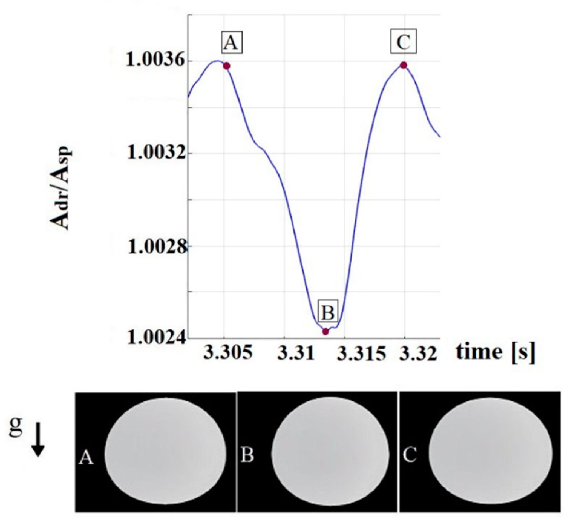
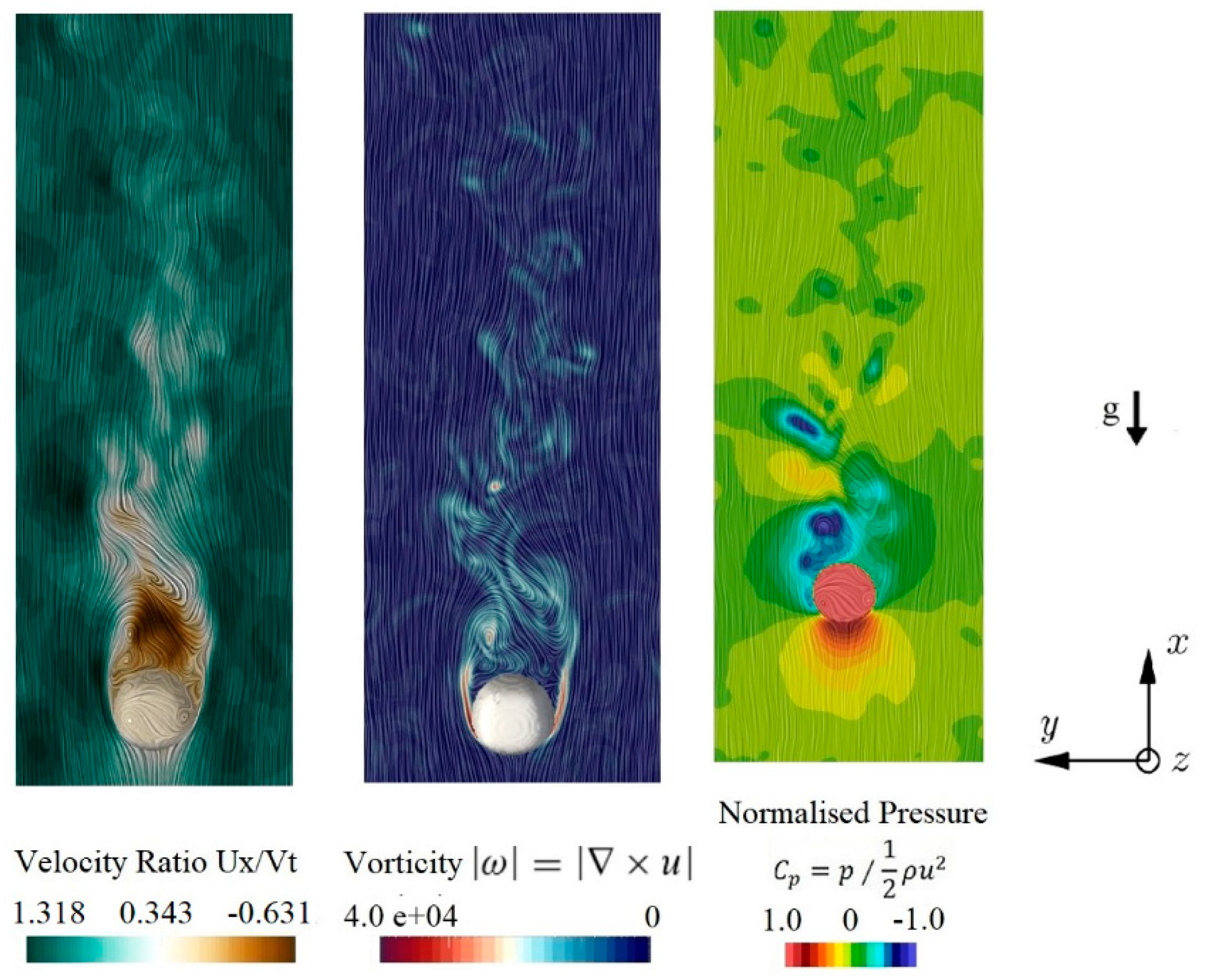
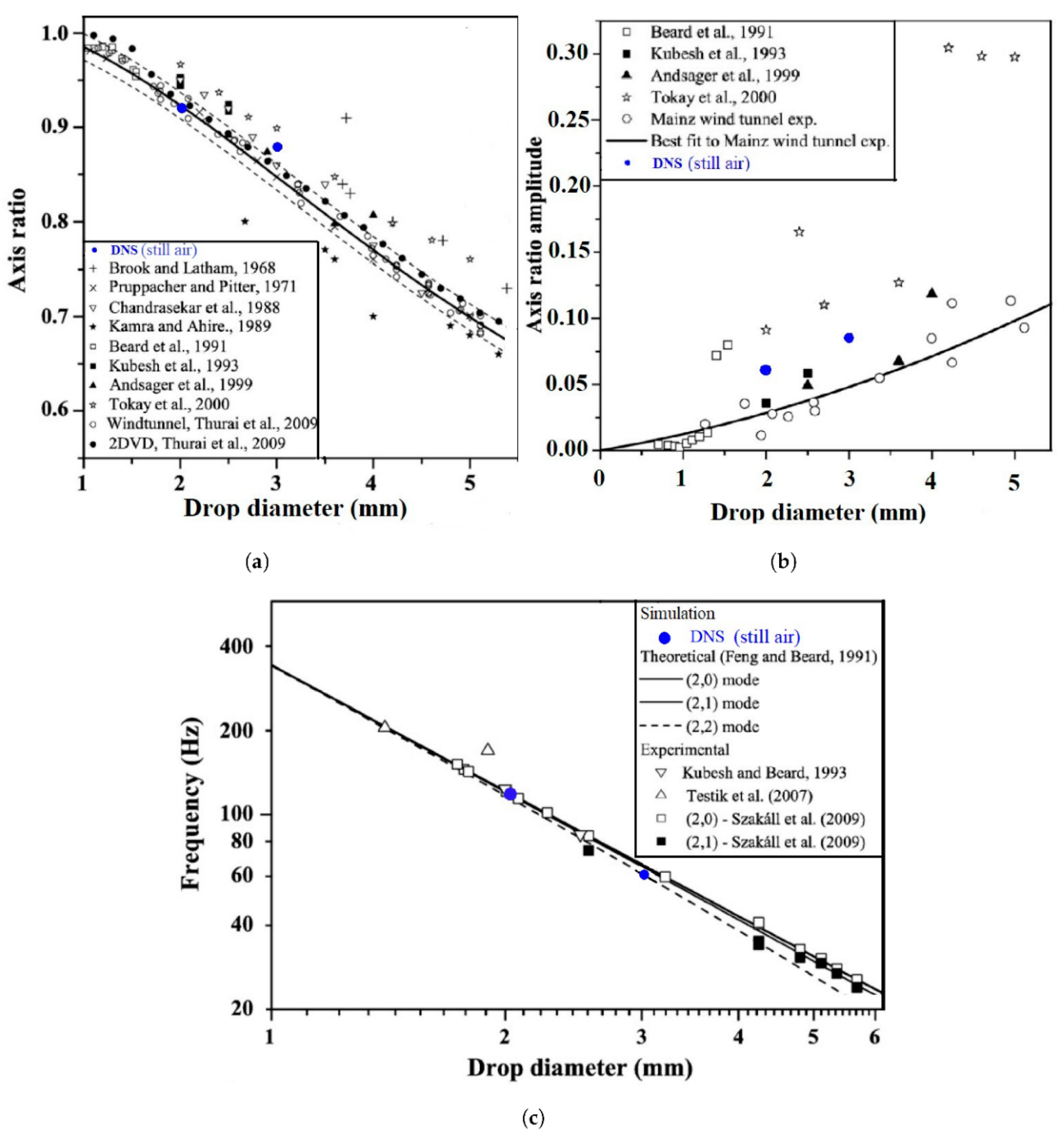
A theoretical study of the flow fields around falling water drops with diameters larger than 1 mm was only recently performed by Ren et al. [34]. They performed calculations to determine the impact of turbulence on the terminal velocity of 2 and 3 mm water drops. They used the Navier–Stokes equation solver FE3D [35] to obtain the flow field and acquired the volume of the fluid [36] with piecewise linear interface calculation (PLIC [37]) to take care of the shape change and oscillation. Their results demonstrated that the flow fields can be simulated reasonably well, including the effects of shape change and oscillation during the fall (Figure 3 and Figure 4).

Ren et al. [34] showed that their results correlate well with experimental data on the drop terminal velocities and shape, as described by Pruppacher and Beard [38] and Beard [39], as well as data on drop oscillations, as described by the field observation by Tokay and Beard [40] and Szakall et al. [21]. These comparisons are shown in Figure 5.

4. Ice Particles

4.1. Observations of Ice Particle Fall Attitudes

Ice particles can be present in clouds where the temperature is below freezing, although many clouds remain completely liquid (albeit supercooled) under this condition [2]. The ice particles in clouds can be divided into four general types. (1) Ice crystals—single ice crystals that are either pristine or rimed. Such single ice crystals are usually called snow crystals when they fall to the surface. (2) Snowflakes—also called snow aggregates, they are formed by the collision and coalescence of many single ice crystals with numbers ranging from a few to over 100. (3) Graupel—these are rimed particles formed by the collision and subsequent freezing of supercooled drops with ice crystals. Their shape is often conical. In cloud physics, a graupel should be smaller than 5 mm in size by definition. (4) Hailstones—these are also rimed particles but with sizes larger than 5 mm and can be larger than 10 cm.

A systematic scientific investigation of the kinematic properties of falling ice particles only started in the 20th century and Japanese scientists appeared to be very early in this endeavor. Nakaya and Terada [41] performed simultaneous observations of the mass, fall velocity, and form of individual snow crystals. Magono [42,43,44] measured the fall velocity of both single crystals and snow aggregates, and theoretical interpretation of the measured fall velocities of planar, dendritic, spatial, and needle crystals; graupel; and snowflakes. Further studies on the fall velocity as well as fall attitude of snow were made by Litvinov [45], Bashkirova and Pershina [46], Jayaweera and Mason [47], Jayaweera and Cottis [48], Magono and Nakamura [49], Podzimek [50,51], Fukuta [52], Brown [53], Jiusto and Bothworth [54], Heymsfield [55], and Jayaweera and Ryan [56] made further investigations on the velocity and attitude of falling snow particles or simulated ice particles.

Ice crystals can be pristine or rimed. One of the most comprehensive studies of the fall attitudes of rimed ice crystals was performed by Zikmunda and Vali [57] who investigated the fall patterns and velocities of rimed ice crystals, sized between 0.02 to 0.5 cm, and determined the relationships between terminal fall velocities and crystal dimensions for graupel, rimed columnar crystals, rimed plate crystals, rimed capped columns, rimed broken branches, and aggregates of rimed crystals. Their results concerning the fall of ice crystals are summarized by Wang [58] (Chapter 2).

Kajikawa [59] measured the fall velocity of individual unrimed snow crystals. His results show that the fall velocity of ice crystals varies with crystal habit and apparently the higher-density ones (such as thick plates and regular plates) fall much faster than lower-density ones (such as dendrites and stellar crystals) for a given size, which coincides with our common sense but in a quantitative way. Many more such observations were subsequently made by Kajikawa [60,61,62,63,64,65] for the falling motion of graupel and snowflakes in addition to ice crystals. Recently, Westbrook and Sephton [66] utilized the 3-D printing technique to produce analogues of complex ice particles to investigate their fall speeds and orientations in the laboratory.

We now discuss the observational studies of the fall attitude of graupel and hailstones. Magono [43] observed that the graupel can fall in oblique orientation on its way down. List and Schemenauer [67] performed laboratory observations on the free-fall behavior of man-made models of planar snow crystals, conical graupel, and conical small-hail particles in glycerin–water mixtures and salt solutions. They observed that the conical models have two types of quasi-periodic oscillations: a sideways oscillation of the center of mass with a frequency of ~0.2 Hz and amplitudes up to 1–2 particle diameters, and an angular oscillation or swinging of the axis of rotational symmetry with a frequency ranging from 0.1 to 1 Hz. They also found that the 90° teardrop-shaped model can fall stably in a sideways position, independent of the position of release. However, tumbling is reported at higher Reynolds numbers when released in the apex-down position because the teardrop model carries out one or more complete rotations to reach a stable sideways position. This peculiar alignment of the particle axis could explain why an ellipsoidal hailstone often contains a conical embryo particle with its main axis oriented at a right angle to the hailstone’s stable fall direction, a direction parallel to its smallest axis. The 90° cone-spherical sector is more stable, falling in the base-down orientation, while the 70° cone-spherical sector is more stable, falling in the apex-down orientation. The latter represents the most stable combination of model and position for Re < 1000. The former combination, however, never shows oscillations >30° with an occurrence of more than 50%, even at Re > 1000. The 90° cone-hemisphere is more stable, falling in the base-down orientation. A discussion of the origin of the oscillations cannot be carried out here, as these secondary motions will be connected with the still-unknown shedding of vortices in the wakes of the models or special boundary effects. In addition, it has to be pointed out that the stability situation for atmospheric particles may also be affected by a nonhomogeneous density distribution within single hydrometeors.

Zikmunda and Vali [57] also made observations of the fall attitude of graupel. They observed that lump graupel falls mostly in a steady manner, whereas conical graupel most frequently exhibits oscillations of the major axis in the vertical direction. The mean position of the apex of conical graupel is upward-consistent with the opinion of List [68], but is in contradiction with Magono [43] who held that the oblique position of the major axis was the stable fall attitude.

Pflaum et al. [69] performed a vertical wind tunnel study on the hydrodynamic behavior of growing, freely falling graupel. They grew the graupel, with a diameter of 200–600 μm, from an initial frozen drop suspended in the wind tunnel. The final size of the graupel was 800 μm–1.2 mm in diameter. The supercooled drops had a diameter ranging 8–30 μm, with a peak at 14 μm. They observed the following five basic fall modes: (1) rotational (spinning) motion around the ice particle’s vertical axis; (2) helical translator motion; (3) a ‘bell-swing’ or ‘pendulum-swing’ type of oscillatory motion; (4) precession of the axis of rotation; and (5) quiescent fall. No tumbling motions, i.e., motions during which the ice particle would rotate by 360” around the axis perpendicular to the fall direction, were observed. Note, however, that Pflaum et al. [69] only observed relatively small graupel. As we will see below, the numerical results show that tumbling will occur when the graupel becomes larger.

Finally, the fall behavior of hailstones will be briefly summarized. Due to their large sizes (up to baseball and grapefruit size) and very high velocities (up to ~40 m s⁻¹), it is very difficult to perform a laboratory study on their fall behavior because no vertical wind tunnel at present has a vertical wind speed comparable to hailstones’ fall speeds. It will also require a very long vertical distance for hailstones to reach terminal velocities, and a very large facility would be needed to conduct drop-tower-type experiments. Due to such difficulties, many hail fall attitude studies were made based on the indirect inference of the hail structure.

List [70] performed a study on the aerodynamics of hailstones based on ellipsoidal model hailstone experiments and found that they fall in the direction of the shortest axis and they fall stably, indicating that no tumbling occurred in the fall. In addition, List et al. [71] found that falling spheroids can oscillate on a horizontal main axis, and can sometimes commence and carry out continuous rotations. The most general motion for a smooth spheroid turned out to be a gyration with the spin around the minor axis which follows the surfaces of a cone. Based on his observations, Lesins and List [72] estimated that the spin and nutation–precession frequencies of gyrating hailstones reach up to 50 Hz. Knight and Knight [73], on the other hand, argued that moderate-to-large hailstones perform rapid symmetrical tumbling during their fall, based on the study on the internal structure of the hailstones.

Recently, there is an enhanced interest in studying the motions of ice particles, possibly because of the importance of high cloud impact on the global climate. Innovative laboratory experimental investigations (e.g., [66,74,75]) or in situ filed observations (e.g., [76]) have been carried out, and there will certainly be more data for ice particle motion studies.

4.2. Flow Fields around Falling Ice Particles

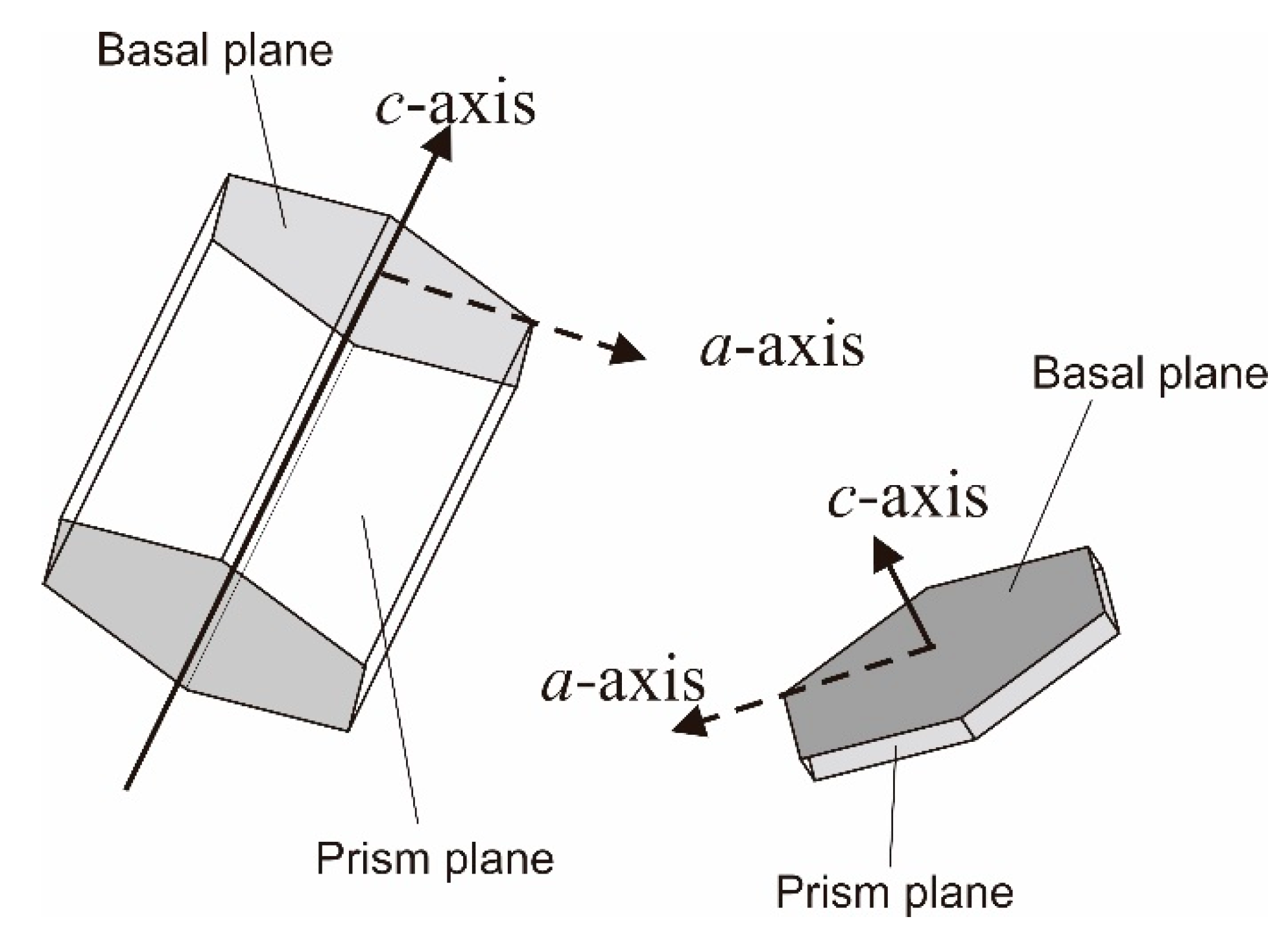
Theoretical studies on the fall motions of ice crystals involve solving the same equation set (2) and (3) with boundary conditions (4) and (5). Unlike the case of small water drops, ice crystals are highly non-spherical, even at very small sizes, apart from frozen drops. The two fundamental ice crystal habits are hexagonal columns (long dimensions along the c-axis) and hexagonal plates (long dimensions along the a-axis) (Figure 6).

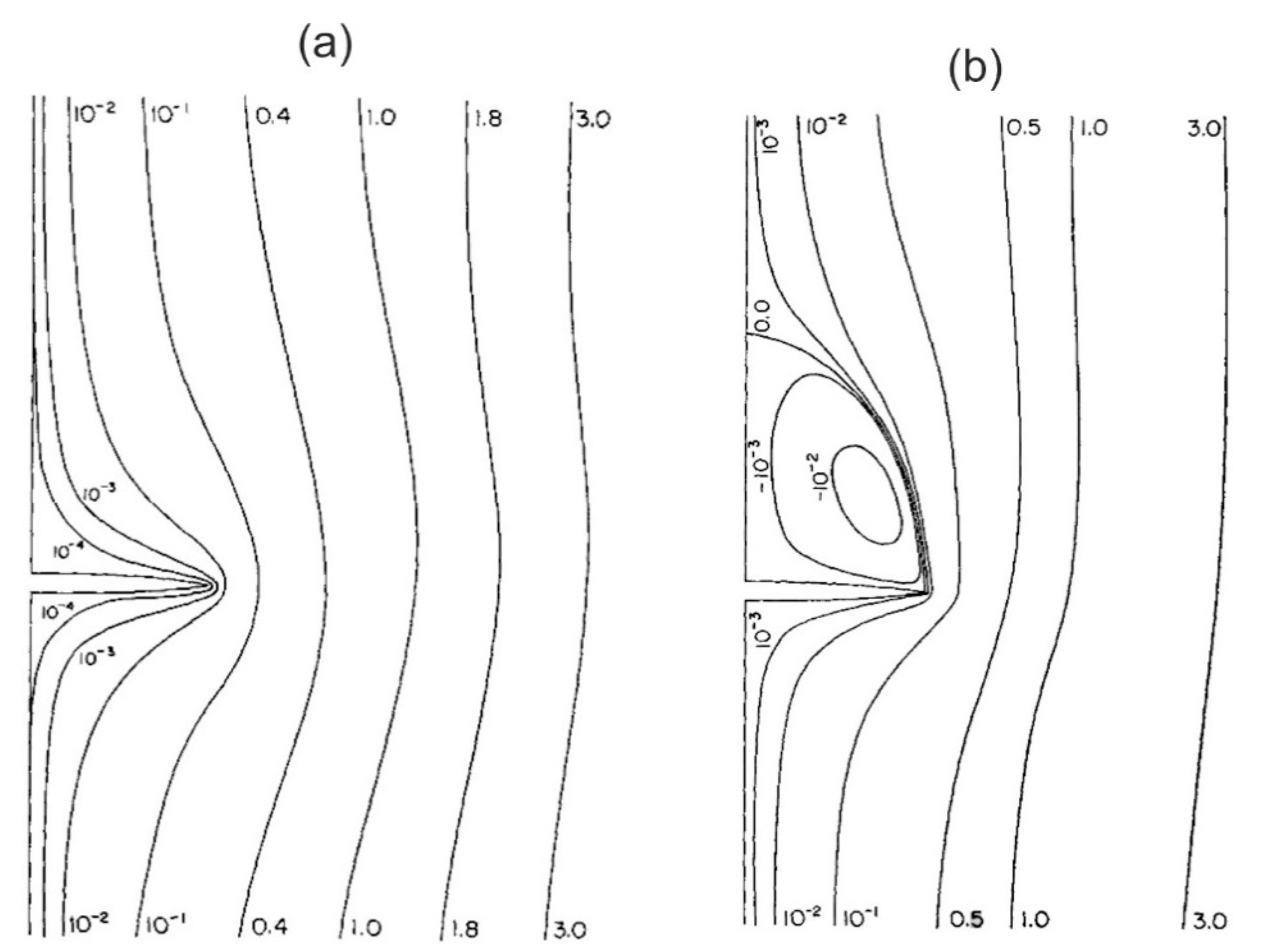
Like the case of water drops, earlier studies of the flow fields around falling ice crystals are confined to either analytical solutions or numerical solutions with crude simplifications. The situation is more difficult for ice particles because most of them are not spherical; hence, even analytical solutions are difficult to obtain, because the symmetry becomes more complex. Consequently, simplifications had to be made, such that the problem can be treated at ease. For example, the flow field of a falling hexagonal ice column was approximated by the flow field around a two-dimensional circular cylinder, and such flow fields were investigated by numerous researchers (e.g., [77,78,79,80,81]). Nevertheless, a two-dimensional cylinder is an infinitely long cylinder in three-dimensional sense; hence, the approximation is indeed very crude, especially when the flow field near the end of a finite length ice column is of concern. Similarly, the flow field around a falling hexagonal ice plate was approximated by the flow around a falling thin oblate spheroid, as investigated by Rimon and Lugt [82], Masliyah and Epstein [83], and Pitter et al. [84]. While this approximation is somewhat better than the situation of the ice column case, in that a thin oblate spheroid is a 3-D object, just like a hexagonal ice plate, it misses on the two sharp edges of a true plate of finite thickness. Still, the resulting flow fields represent reasonable approximations (Figure 7) and lead to useful conclusions of cloud physical processes. For example, the flow fields correctly predicted that the initial riming of ice plate tends to occur at the rim and not at the center [85]. In addition to the crude simplification of particle shapes mentioned above, earlier studies of the flow fields around falling ice particles assumed steady-state conditions, just like the case of [29] for flow around falling water drops. Thus, the shape approximation and steady-state assumption results in the calculated flow fields that are both steady and axisymmetric.

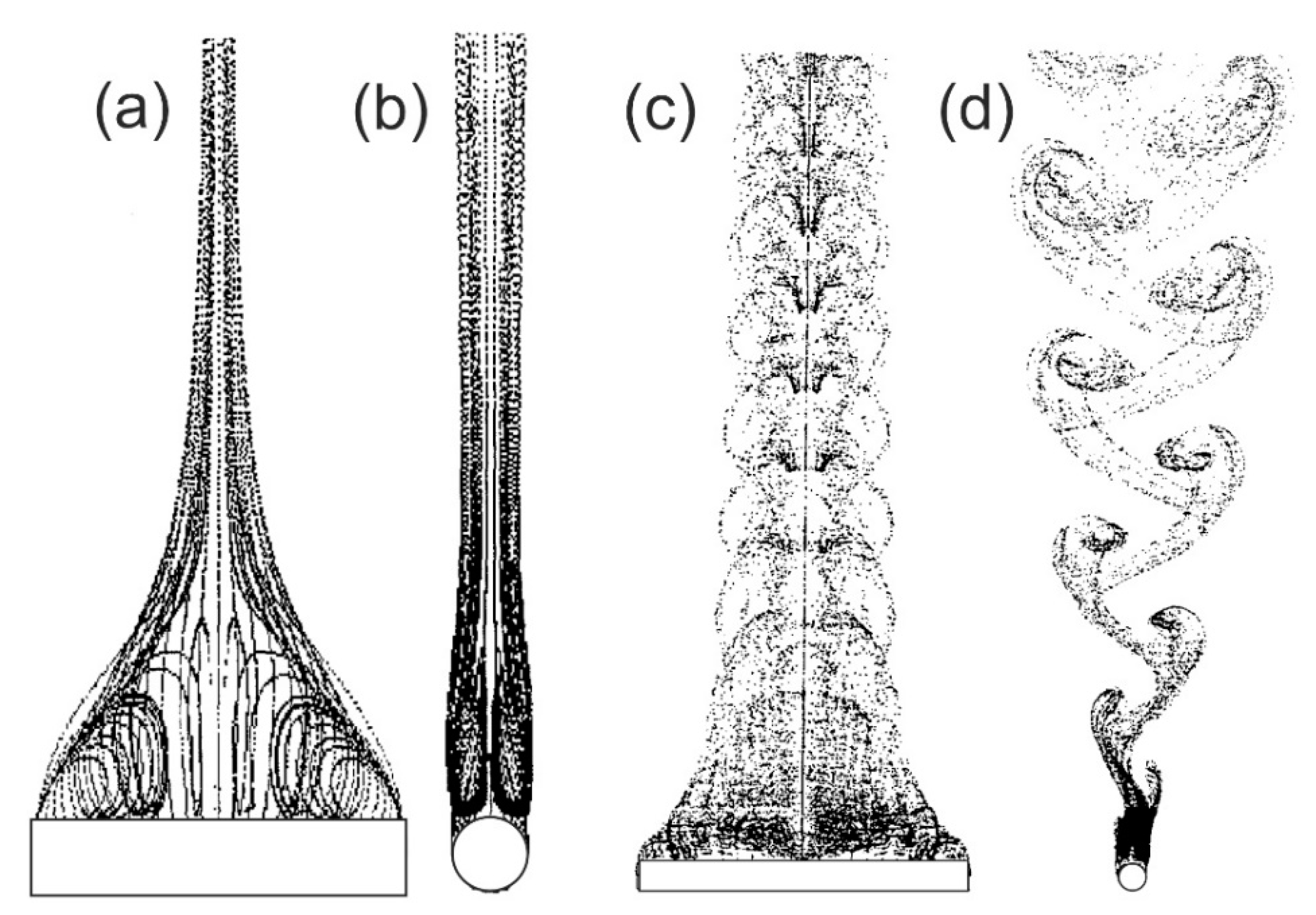
Clearly, the assumptions and simplifications made by these earlier studies were mainly due to the limitation of computing technologies available at the time. This situation was first improved by Ji and Wang [86,87] and Wang and Ji [88] who theoretically determined the flow fields past falling ice columns and places. For the first time, the unsteady flow fields were numerically obtained. Thus, it was the full set of non-steady-state Navier–Stokes equations, i.e., Equations (2) and (3), that is numerically solved instead of the steady-state N-S Equation (9). The shape problem was also improved by Ji and Wang [86] and Wang and Ji [88] who used an exact hexagonal plate with finite thickness to represent the ice plate and a circular cylinder of finite length to represent the hexagonal ice column. Thus, the important unsteady flow characteristic phenomenon, the eddy shedding in the downstream of the falling ice particle, was successfully simulated for the first time (Figure 8). In addition, the formation of the pyramidal wake due to the finite length of the column, which is nonexistent in the case of the fall of a two-dimensional cylinder, as in previous studies, was also captured by this simulation. The results of these simulations agree well with the experimental data of Jayaweera and Mason [47].

However, although the unsteady flow characteristics were successfully simulated, these new studies still suffered from two shortcomings. First, the ice columns and plates were assumed to fall straight perpendicular to their largest dimension, i.e., the column falls with a horizontally oriented length and the plate with a vertically facing basal plane [1]. Part of the reason why vertical orientation was assumed in early studies is because of the ease in forming the numerical mesh for the finite difference calculations. While this assumption may be acceptable when the ice crystals are small, it is well known that large ice crystals can change their orientations significantly with respect to the vertical during the fall. Second, the ice crystal was assumed to fall along a vertical line; thus, horizontal translational motions were prohibited. Yet, it is well known that ice crystals will perform complex fall attitudes that include substantial horizontal translation when they are large enough.

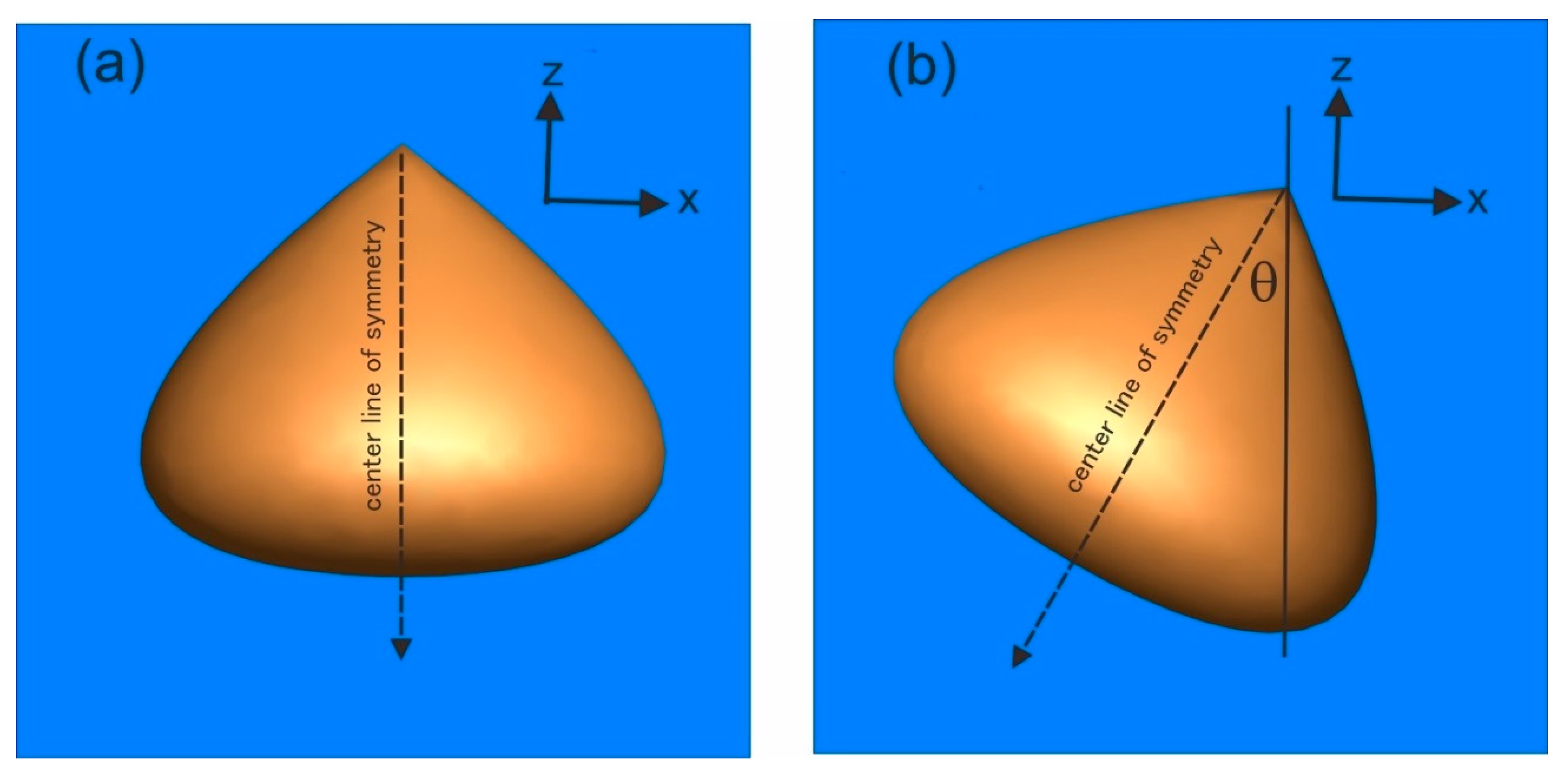
Kubicek and Wang [89] and Wang and Kubicek [90] improved the assumption of vertical fall orientation by allowing the fall orientation of an ice particle to be tilted with respect to the vertical. They used Wang’s mathematical expression [91] to generate the conical graupel and studied the fall of conical graupel, whose apices are oriented in various angles with respect to the vertical. The definition of the center line of symmetry (CLS) is shown in Figure 9.

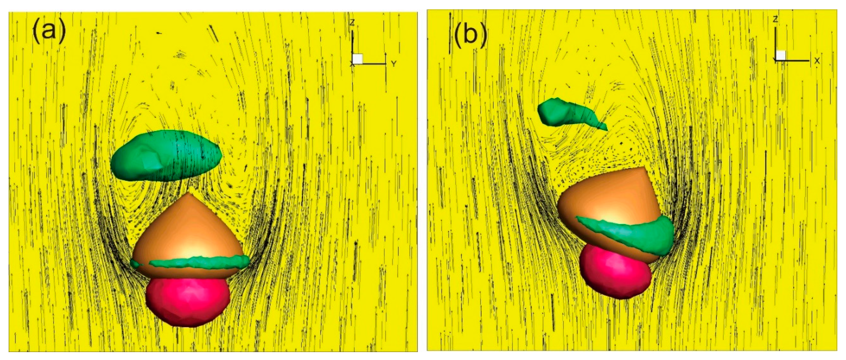
All previous theoretical studies on the fall of ice hydrometeors assume that CLS is aligned with the vertical, and the study of Kubicek and Wang [89] was the first one to allow the CLS to orient at an arbitrary angle with respect to the vertical (Figure 10b). They utilized Fluent, the computational fluid dynamics (CFDs) package (later changed to the name ANSYS), as the non-steady-state Navier–Stokes equation solver to obtain the flow field around a falling conical graupel.

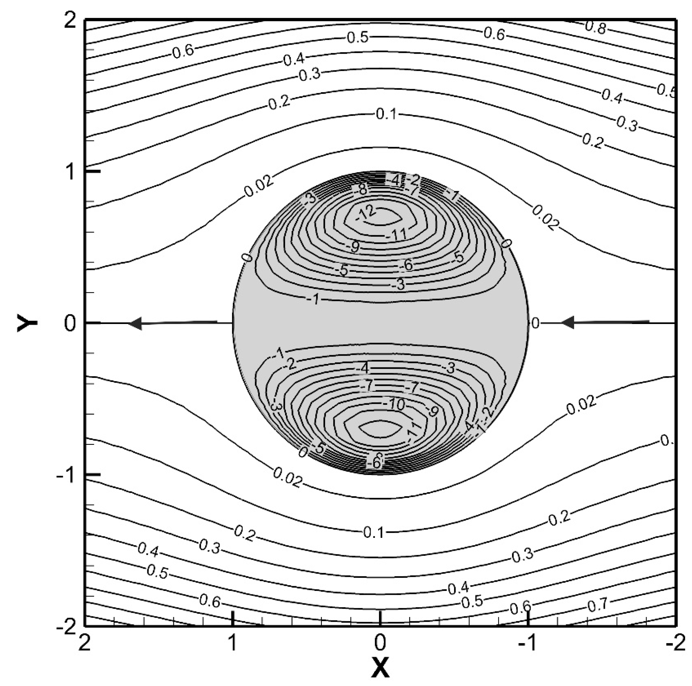
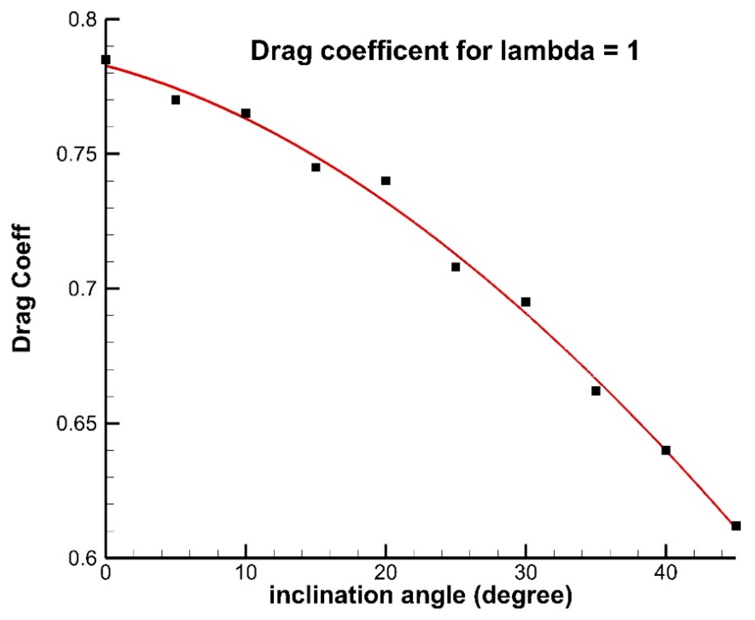
Figure 10 shows the flow field and high- and low-pressure regions around a falling conical graupel of 3 mm diameter, taken from the output produced by Kubicek and Wang [89]. Figure 11 shows the drag coefficients derived from the study by them. It demonstrated that the tilted fall attitude of a conical particle has a significant impact on the flow field and the derived hydrodynamic properties (such as drag), thus underlying the necessity of investigating the impact of the tilted fall attitude.

Still, the conical graupel in Kubicek and Wang’s study [89] did not remove the shortcoming of restricting the fall to be on a straight vertical line. A similar study was performed by Hashino et al. [92] to investigate the fall of hexagonal ice columns with inclined orientations, again allowing only the fall path to be a straight vertical line.

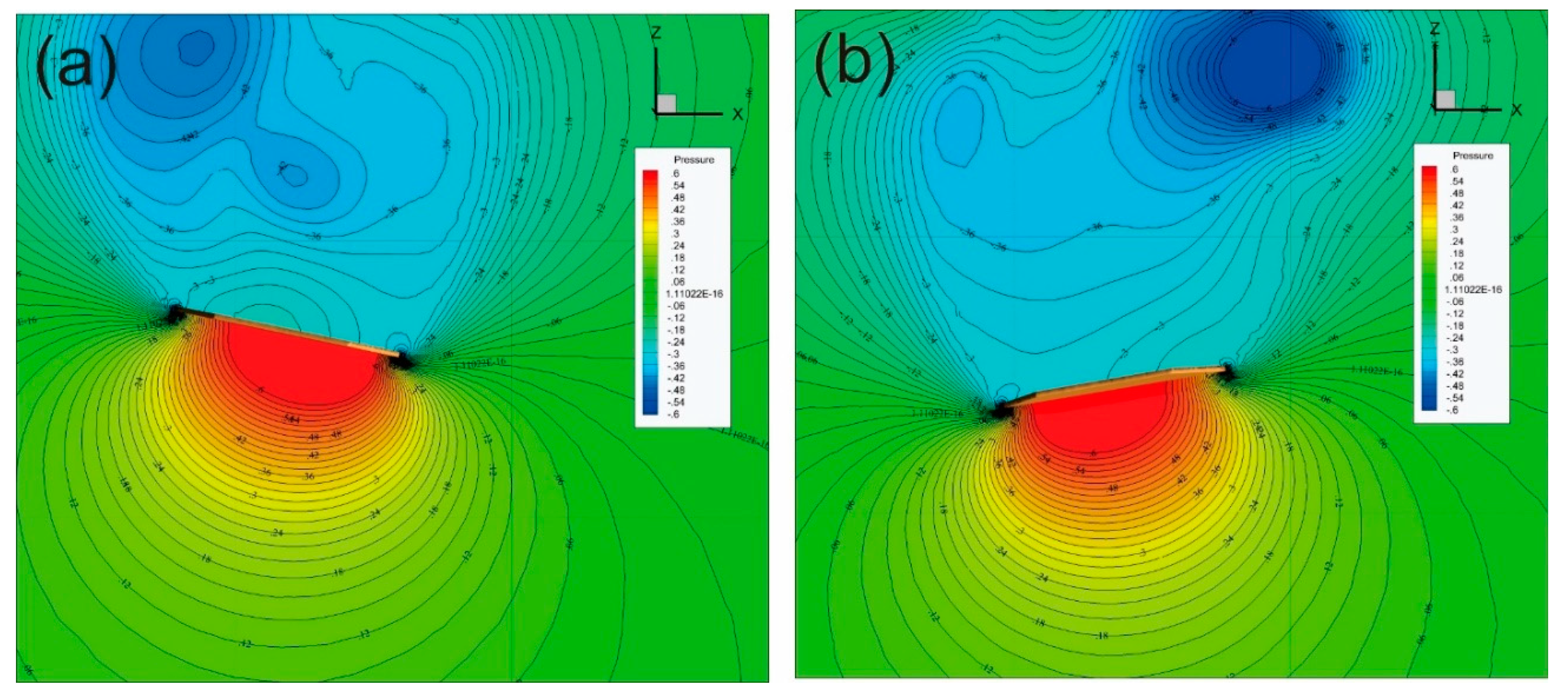
This restriction was finally removed by Cheng et al. [93] who investigated the free-fall behavior of hexagonal ice plates using ANSYS software. In order to allow both the horizontal translational motions but also the change in posture of the falling ice plate, they utilized the 6 degrees of freedom option in ANSYS, such that there was a need to regenerate the finite volume numerical mesh at each step to accommodate the changes in both the crystal position and the posture. This required a substantial computing resource, but produced highly successful results. The numerical simulation not only produced very reasonable instantaneous flow fields around the plate (Figure 12) and realistic zig-zag horizontal motions during the fall, but also simulated the expected changes in posture, as revealed by the Tait–Bryan angles. Ice plates also exhibit rotation in the c-axis during the fall, as one would expect such a mode to occur in the falling hexagonal plate.

Figure 13 shows the combined individual snapshots of the falling hexagonal plate at all time steps in the simulation in three different view directions. We shall call this type of plots “trajectoroid” for convenience, representing more or less the trajectory of each point on the plate surface throughout the simulation. The trajectoroid not only reveals the trajectories but also the instantaneous posture of the falling plate. In Figure 13, we see that the plate not only performs a zig-zag fall attitude and horizontal translation, but also some small rotation in the c-axis of the crystal. The most obvious of these motion modes is the y-z plane view, as shown in Figure 13c. All derived hydrodynamic properties of the simulated fall of these hexagonal plates agree fairly well with observational or experimental data. We believe that Cheng et al. [93] is the first successful numerical simulation of the true free fall of ice crystals as it facilitates the interaction of the flow field and the adjustment of the plate.

Following the successful work of Cheng et al. [93], Hashino et al. [94] performed a study to understand the falling patterns of relatively large hexagonal columnar crystals (Re = 10 to 193.7), utilizing the same CFD package Fluent. Aside from their fundamental importance in cloud physics, columnar ice crystals play an important role in atmospheric radiation, such as the formation of halo in cirrostratus clouds, and a good understanding of their motion modes, which helps to clarify some observed optical phenomena associated with high clouds. Hashino et al. [94] found that there are three modes of fall patterns, namely strong damping, fluttering, and instability. They further found that the strong damping mode is the most likely to occur in the atmosphere, but the fluttering mode is also possible. On the other hand, the unstable mode is most unlikely to happen in the atmosphere.

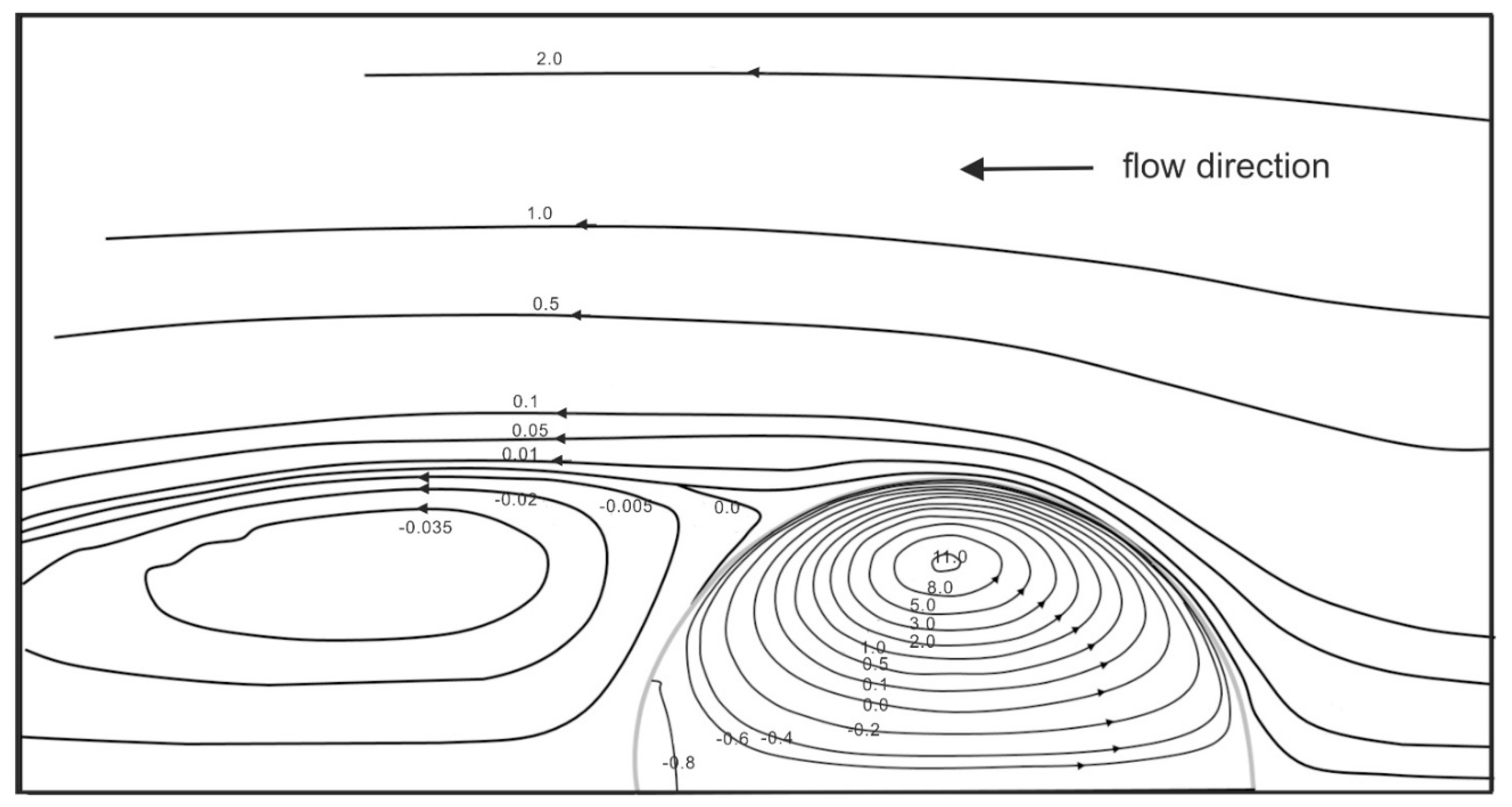
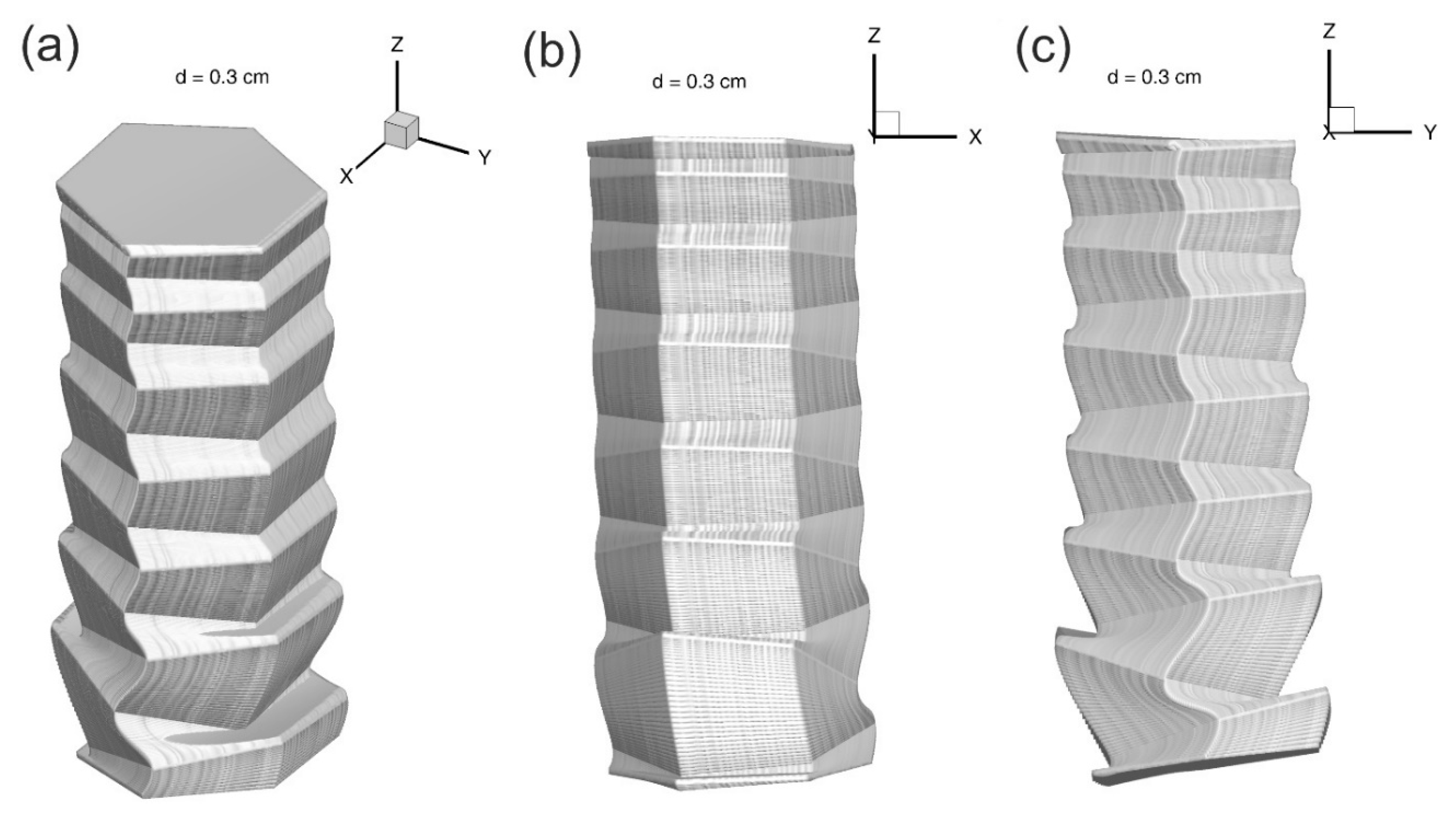
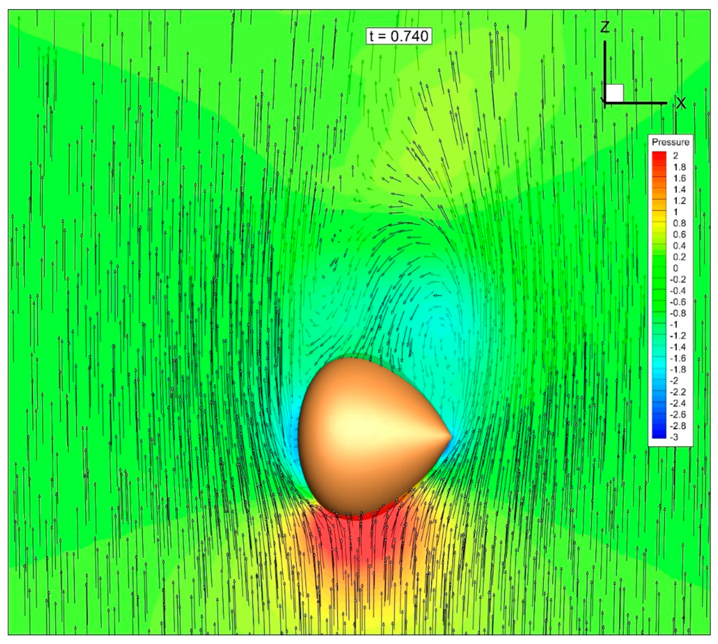
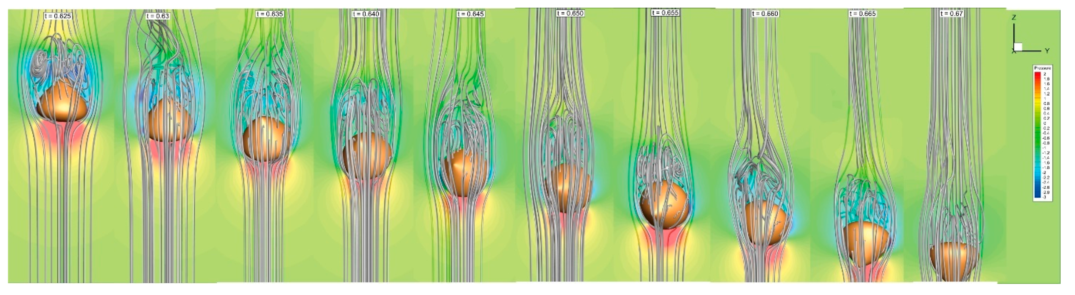
Similar works were performed by Chueh et al. [95,96] who studied the motions of conical graupel freely falling in the atmosphere. Graupel plays a very important role in many aspects of cloud physics, especially as the precursor of hailstones that can produce severe damage to crops and properties and possibly human injuries. Secondly, collision between graupel and ice crystals is currently considered as the major electrification mechanism of thunderclouds [2,97]; hence, their hydrodynamic behavior can have a great impact on deep convective cloud physics. Most heavy precipitation in convective clouds is related to graupel [98]. The collection efficiency of drops by graupel particles is a key source of uncertainty [99]. Chueh et al.’s results [96] exhibit all the complex modes of motion of conical graupel during the free fall, as shown by Pflaum et al. [69]’s laboratory experiment. These modes include spiral fall path, pendulum swing, precession, rotation, and tumbling, which all occurred at appropriate Reynolds number ranges, as observed. Figure 14 shows a typical flow field of the freely falling conical graupel obtained by Chueh et al. [96], and Figure 15 shows a sequence of flow fields expressed by the stream traces of a freely falling conical graupel which performed a tumble from an apex-upright posture to an apex-down posture in a period of 0.045 s.

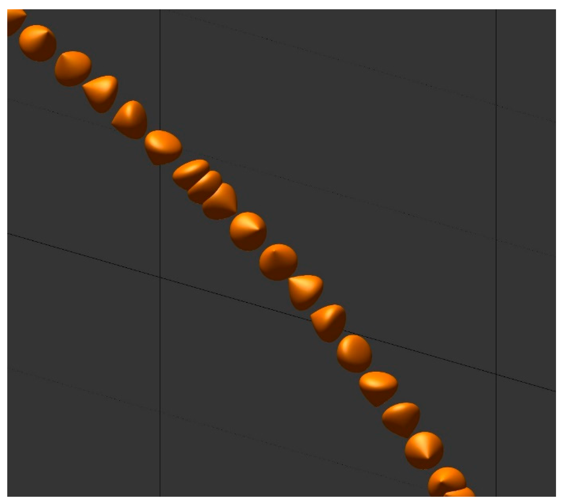
One interesting feature of the free fall of conical graupel studied by Chueh et al. [96] is that once a graupel starts to tumble, it tends to continue tumbling and move in a more-or-less unchanged direction throughout the simulation period, albeit with some spiraling (Figure 16). Such a motion behavior makes it possible for graupel to spread to a very wide range within the cloud, possibly wider than any other types of hydrometeors. This is quite in contrast to the case of ice crystals, which tend to zig-zag in a limited range of horizontal movement (see, e.g., the ice plate in Figure 13). The implications of this behavior on cloud physics are yet to be studied.

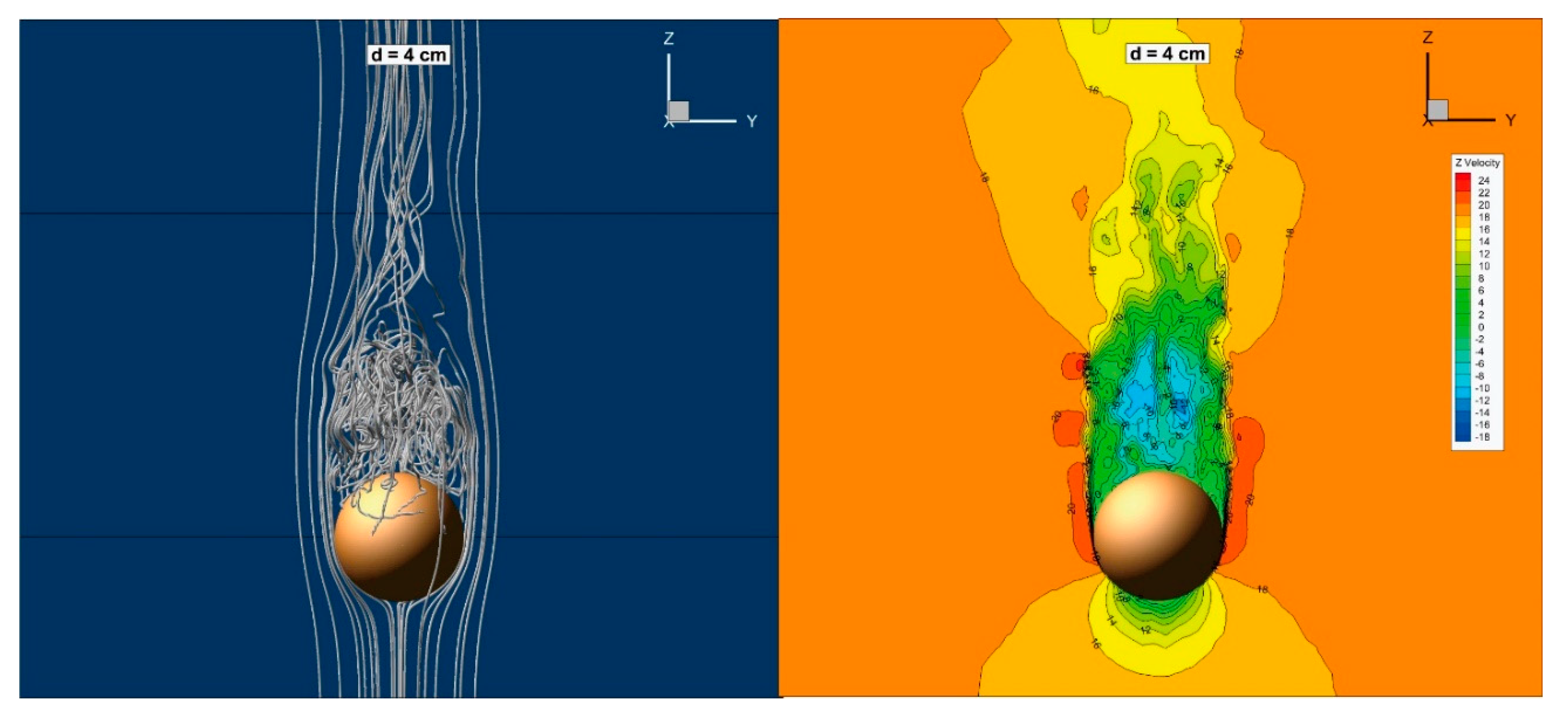
Another type of rimed ice hydrometeor freely falling in the atmosphere, hailstones, has been studied by Cheng and Wang [100], with the assumption that hailstones can be approximated by smooth spheres with diameters ranging from 1 to 10 cm, corresponding to a Reynolds number range from 5780 to 206,000. Before that, the largest spherical hydrometeor subject to numerical flow field simulation was a spherical water drop with a diameter of 876 μm performed by Grover et al. [101] who studied the water drop scavenging of aerosol particles. The spheres of hailstones with varying sizes induce highly unsteady flow fields, and it was difficult to carry out numerical studies in earlier times due to the limitations of computing resource and technology. Advancements in computing technology allowed Cheng and Wang [100] to perform numerical simulations of falling spherical hailstones utilizing the ANSYS CFD package. Later, a similar study by Wang et al. [102] sought to extend Cheng and Wang’s work [100] to simulate the fall of lobed hailstones with a Reynolds number ranging from 9560 to 388,000. Both simulations of smooth and lobed spheres were successful, and an example of the flow fields in these studies is shown in Figure 17.

More recently, Nettesheim and Wang [103] followed Cheng et al. [93] and Hashino et al.’s [94] line of work to extend the flow field simulation to more general forms of ice crystals, such as broad branch crystals (BBCs), stellar crystals, and ordinary dendrites, which also exist in natural clouds. Their fall behaviors are similar to those of hexagonal plates, and the trajectories in Figure 18 show an example of a falling BBC with a diameter of 5 mm.

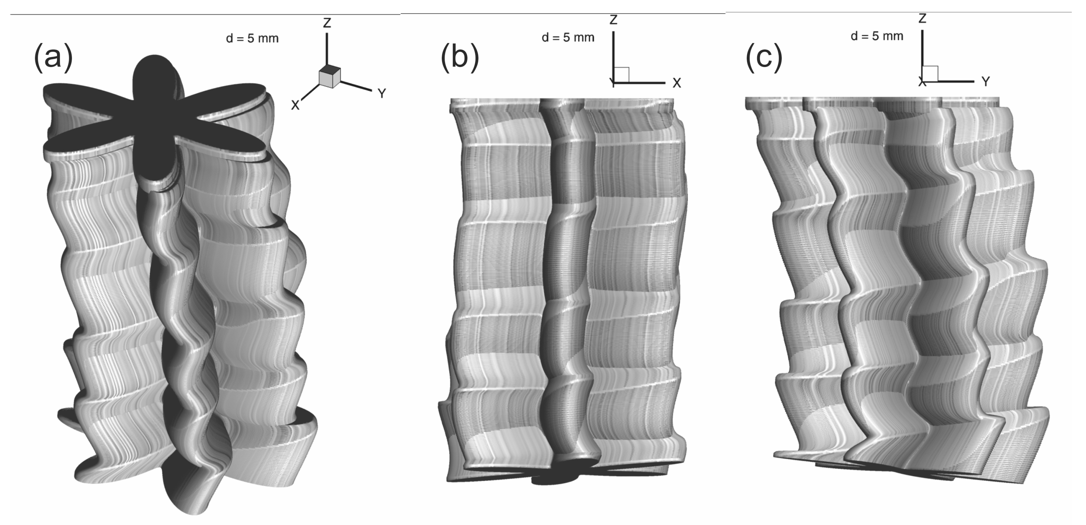
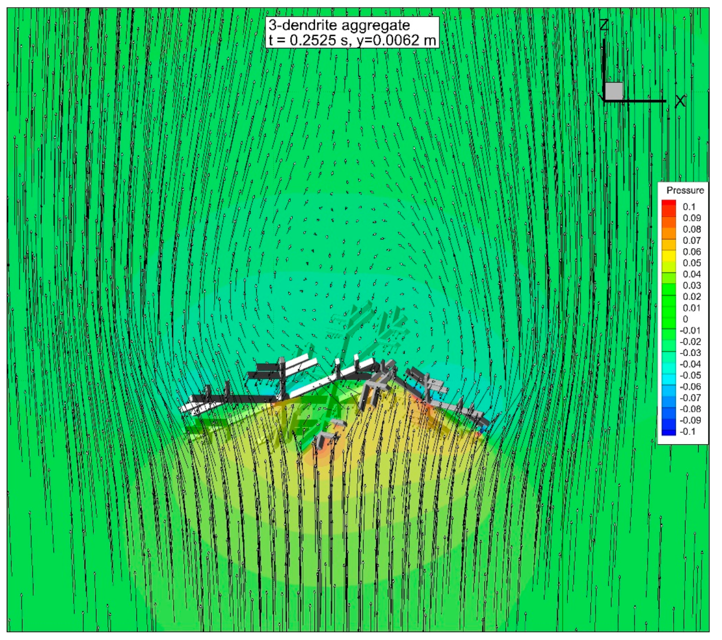
In the above discussions of the fall of ice crystals, only a single crystal was considered. More recently, work has begun on the motion of snow aggregate, as this is one area that has not received detailed investigation. This is obviously due to the complex shape of snow aggregates (or simply snowflakes) because they are formed by the collision and coalescence of individual ice crystals that can be of different sizes and crystal habits. In previous investigations of flow past ice crystals, the requirement of computing resource was already quite demanding. Nevertheless, some preliminary results have been obtained by Wang [58].

Figure 19 shows an example taken from that study. It shows the velocity and pressure field in a vertical cross-section around a freely falling snow aggregate consisting of three individual conformal dendrites, but of different sizes. From this preliminary example, it is easy to see the complex shape; hence, the required computing resource is considerable. However, this project is ongoing and will be completed soon.

5. Summary and Outlook

A brief review was performed on the theoretical (mainly numerical) studies of the flow of hydrometeors falling in the atmosphere. The hydrometeors reviewed include cloud drops, rain drops, small pristine ice crystals, large pristine ice crystals, snow aggregates, conical graupel, and smooth and lobed spherical hailstones. We focused on the theoretical studies that aimed to solve the relevant Navier–Stokes equations, so that the detailed flow fields (velocity, pressure, vorticity, etc.) around the falling hydrometeors are completely determined.

There are still gaps in this research area. One area that should be completed in the near future is the flow fields around falling snowflakes that consist of many ice crystals. The example demonstrated in Figure 17 consists of three crystals of the same habit (all are ordinary dendrites). Future calculations should be performed for more numbers of crystals. The necessity of involving different crystal habits remains to be studied, as flakes consisting of many crystals of one habit already have very complex surface morphology whose fluid dynamic properties would probably hardly change, even if a flake is made of crystals of other habits.

The second important gap to be filled is the calculations of the flow around rimed ice particles. All the theoretical flow fields around falling ice crystals are for clean, or pristine, crystal cases. However, rimed ice crystals play an important role in precipitation physics as they are the intermediate stage between cloud and precipitation particles, especially in the formation of graupel and hailstones, although some rimed crystals melt to form raindrops. In addition, the graupel and hailstones mentioned in the previous sections are assumed to have smooth surfaces, but in reality, many of them would be heavily rimed on the surface. These large rough-surfaced ice particles may have a great impact on the dynamics of severe storms, and their fall behavior must be studied.

Another important gap is the simulation of the complete free fall of large rain drops associated with unsteady fall behavior such as canting and breakup, with the latter mostly occuring during the collision of two or more drops, which plays an important role in deciding the raindrop size spectrum when drops approach the ground.

Finally, a highly challenging and yet also very important area of future research in this direction is the study of the free fall of large mixed-phase particles, i.e., partially melted ice particles. Their fall behaviors are highly complicated, as demonstrated by the wind tunnel experiments of Rasmussen et al. [104]. A quantitative description of the fall behavior with detailed flow and thermodynamic fields will be necessary for a complete understanding of severe storm dynamics.

References

- Pruppacher, H.R.; Klett, J.D. Microphysics of Clouds and Precipitation, 2nd ed.; Springer: Dordrecht, The Netherlands, 1997; ISBN 978-0-7923-4211-3. [Google Scholar]
- Wang, P.K. Physics and Dynamics of Clouds and Precipitation; Cambridge University Press: Cambridge, UK, 2013; ISBN 9780511794285. [Google Scholar]
- Beard, K.V.; Pruppacher, H.R. A wind tunnel investigation of collection ker-nels for small water drops in the air. Q. J. R. Meteorol. Soc. 1971, 97, 242–248. [Google Scholar] [CrossRef]
- Beard, K.V.; Pruppacher, H.R. An experimental test of theoret-ically calculated collision efficiencies of cloud drops. J. Geophys. Res. 1968, 73, 6407–6414. [Google Scholar] [CrossRef]
- Hockings, L.M. The collision efficiency of small drops. Q. J. R. Meteorol. Soc. 1959, 85, 44–50. [Google Scholar] [CrossRef]
- Hockings, L.M.; Jonas, P.R. The collision efficiency of small drops. Q. J. R. Meteorol. Soc. 1970, 96, 722–729. [Google Scholar] [CrossRef]
- Jonas, P.R. The collision efficiency of small drops. Q. J. R. Meteorol. Soc. 1972, 98, 681–683. [Google Scholar] [CrossRef]
- Pinsky, M.; Khain, A.; Shapiro, M. Collision Efficiency of Drops in a Wide Range of Reynolds Numbers: Effects of Pressure on Spectrum Evolution. J. Atmos. Sci. 2001, 58, 742–764. [Google Scholar] [CrossRef]
- Cotton, W.R.; Bryan, G.; van den Heever, S.C. (Eds.) Storm and Cloud Dynamics, 2nd ed.; Academic Press: Cambridge, MA, USA, 2010; ISBN 9780120885428. [Google Scholar]
- Blanchard, D.C. The behavior of water drops at terminal velocity in air. Trans. Am. Geophys. Union 1950, 31, 836–842. [Google Scholar] [CrossRef]
- Komabayashi, M.; Gonda, T.; Isono, K. Lifetime of water drops before breaking and size distribution of fragment drops. J. Meteorol. Soc. Jpn. 1964, 42, 330–340. [Google Scholar] [CrossRef] [Green Version]
- Cotton, W.; Gokhale, N.R. Collision, coalescence, and break-up of large water drops in a vertical wind tunnel. J. Geophys. Res. 1967, 72, 4041–4049. [Google Scholar] [CrossRef]
- Spengler, J.D.; Gokhale, N.R. A large, vertical wind tunnel for hydrometeor studies. In Proceedings of the Second National Conference on Weather Modification of the American Meteorological Society, Santa Barbara, CA, USA., 6–9 April 1970; pp. 289–293. [Google Scholar]
- Pruppacher, H.R.; Neiburger, M. The UCLA cloud tunnel. In Proceedings of the International Conference on Cloud Physics, Toronto, ON, Canada, 26–30 August 1968; pp. 389–392. [Google Scholar]
- Beard, K.V.; Pruppacher, H.R. A determination of the terminal velocity and drag of small water drops by means of a wind tunnel. J. Atmos. Sci. 1969, 26, 1066–1072. [Google Scholar] [CrossRef] [Green Version]
- Montgomery, D.N.; Dawson, G.A. Collisional charging of water drops. J. Geophys. Res. 1969, 74, 962–972. [Google Scholar] [CrossRef]
- Gunn, R.; Kinzer, G.D. The Terminal Velocity of Fall for Water Drops in Stagnant Air. J. Meteorol. 1949, 6, 243–248. [Google Scholar] [CrossRef] [Green Version]
- Chowdhury, M.N.; Testik, F.Y.; Hornack, M.C.; Khan, A.A. Free fall of water drops in laboratory rainfall simulations. Atmos. Res. 2016, 168, 158–168. [Google Scholar] [CrossRef] [Green Version]
- Sartor, J.D.; Abbott, C.E. Prediction and measurement of the accelerated motion of water drops in air. J. Appl. Meteorol. 1975, 14, 232–239. [Google Scholar] [CrossRef] [Green Version]
- Diehl, K.; Mitra, S.K.; Szakáll, M.; von Blohn, N.; Borrmann, S.; Pruppacher, H.R. The Mainz vertical wind tunnel facility–A review of 25 years of laboratory experiments on cloud physics and chemistry. In Wind Tunnels: Aerodynamics, Models and Experiments; Pereira, J.D., Ed.; Nova Science Publishers: Hauppauge, NY, USA, 2011; pp. 69–92. [Google Scholar]
- Szakáll, M.; Diehl, K.; Mitra, S.; Borrmann, S.A. Wind tunnel study on the shape, oscillation, and internal circulation of large raindrops with sizes between 2.5 and 7.5 mm. J. Atmos. Sci. 2009, 66, 755–765. [Google Scholar] [CrossRef]
- Szakáll, M.; Mitra, S.; Diehl, K.; Borrmann, S.A. Shapes and oscillations of falling raindrops—A review. Atmos. Res. 2010, 97, 416–425. [Google Scholar] [CrossRef]
- Wang, P.K.; Pruppacher, H.R. Acceleration to Terminal Velocity of Cloud and Rain Drops. J. Appl. Meteorol. 1977, 16, 275–280. [Google Scholar] [CrossRef] [Green Version]
- Abbott, C.E.; Cannon, T.W. A drop generator with electronic control of size, production rate, and charge. Rev. Sci. Instrum. 1972, 43, 1313–1317. [Google Scholar] [CrossRef]
- Hadamard, J.S. Mouvement permanent lent d’une sphere liquide et visqueuse dans un liquide visqueux. CR Hebd. Seances Acad. Sci. 1911, 152, 1735–1738. (In French) [Google Scholar]
- Rybczynsky, W. Über die Fortschreitende Bewegung Einer Flüssigen Kugel in Einem Zähen Medium. Bull. Acad. Sci. Cracovie 1911, 1, 40–46. (In German) [Google Scholar]
- Maxworthy, T. Accurate measurements of sphere drag at low Reynolds numbers. J. Fluid Mech. 1965, 23, 369–372. [Google Scholar] [CrossRef]
- Pruppacher, H.R.; Steinberger, E.H. An experimental determination of the drag on a sphere at low Reynolds numbers. J. Appl. Phys. 1968, 39, 4129–4132. [Google Scholar] [CrossRef]
- LeClair, B.P.; Hamielec, A.E.; Pruppacher, H.R.; Hall, W.D. A theoretical and experimental study of the internal circulation in water drops falling at terminal velocity in air. J. Atmos. Sci. 1972, 29, 728–740. [Google Scholar] [CrossRef] [Green Version]
- Hamielec, A.E.; Hoffman, T.W.; Ross, L.L. Numerical solution to the Navier-Stokes equation of motion for flow past spheres. AIChE J. 1967, 13, 213–219. [Google Scholar] [CrossRef]
- Taneda, S. Experimental investigation of the wake behind a sphere at low Reynolds numbers. J. Phys. Soc. Jpn. 1956, 11, 1101–1108. [Google Scholar] [CrossRef]
- Diehl, K. Eine Theoretische und Experimentelle Untersuchung Uber Die Zirkulation in Wolkentropfen und Regentropfen. Diploma Thesis, Institute of Atmospheric Physics, University of Mainz, Mainz, Germany, 1989. [Google Scholar]
- Magarvey, R.H.; Bishop, R.L. Wakes in liquid-liquid systems. Phys. Fluids 1961, 4, 800. [Google Scholar] [CrossRef]
- Ren, W.; Reutzsch, J.; Weigand, B. Direct numerical simulation of water drops in turbulent flow. Fluids 2020, 5, 158. [Google Scholar] [CrossRef]
- Eisenschmidt, K.; Ertl, M.; Gomaa, H.; Kieffer-Roth, C.; Meister, C.; Rauschenberger, P.; Reitzle, M.; Schlottke, K.; Weigand, B. Direct numerical simulations for multiphase flows: An overview of the multiphase code FS3D. Appl. Math. Comput. 2016, 272, 508–517. [Google Scholar] [CrossRef]
- Hirt, C.; Nichols, B. Volume of fluid (VOF) method for the dynamics of free boundaries. J. Comput. Phys. 1981, 39, 201–225. [Google Scholar] [CrossRef]
- Rider, W.J.; Kothe, D.B. Reconstructing volume tracking. J. Comput. Phys. 1998, 141, 112–152. [Google Scholar] [CrossRef] [Green Version]
- Pruppacher, H.R.; Beard, K. A wind tunnel investigation of the internal circulation and shape of water drops falling at terminal velocity in air. Q. J. R. Meteorol. Soc. 1970, 96, 247–256. [Google Scholar] [CrossRef]
- Beard, K.V. Terminal velocity and shape of cloud and precipitation drops aloft. J. Atmos. Sci. 1976, 33, 851–864. [Google Scholar] [CrossRef] [Green Version]
- Tokay, A.; Beard, K.V. A Field Study of Raindrop Oscillations. Part I: Observation of Size Spectra and Evaluation of Oscillation Causes. J. Appl. Meteorol. 1996, 35, 1671–1687. [Google Scholar] [CrossRef]
- Nakaya, U.; Terada, T. Simultaneous Observations of the Mass, Falling Velocity and Form of Individual Snow Crystals. J. Fac. Sci. Hokkaido Univ. 1935, 1, 191–200. [Google Scholar]
- Magono, C. On the fall velocity of snowflakes. J. Meteorol. 1951, 8, 199–200. [Google Scholar] [CrossRef] [Green Version]
- Magono, C. On the growth of snowflakes and graupel. Sci. Rep. Yokohama Nat. Univ. Sect. I 1953, 2, 18–40. [Google Scholar]
- Magono, C. On the falling velocity of solid precipitation elements. Sci. Rep. Yokohama Nat. Univ. Sect. I 1954, 3, 33–40. [Google Scholar]
- Litvinov, I.V. Determination of falling velocity of snow particles. Izv. Akad. Nauk SSR Ser. Geofiz. 1956, 7, 853–856. [Google Scholar]
- Bashkirova, T.A.; Pershina, T.A. On the mass of snow crystals and their fall velocity. Tr. GI. Geofiz. Observ. 1964, 165, 83–100. [Google Scholar]
- Jayaweera, K.O.L.F.; Mason, B.J. The behavior of freely falling cylinders and cones in a viscous fluid. J. Fluid Mech. 1965, 22, 709–720. [Google Scholar] [CrossRef]
- Jayaweera, K.O.L.F.; Cottis, R.E. Fall velocities of plate-like and columnar ice crystals. Q. J. R. Meteorol. Soc. 1969, 95, 203–209. [Google Scholar] [CrossRef]
- Magono, C.; Nakamura, T. Aerodynamic studies of falling snowflakes. J. Meteorol. Soc. Jpn. 1965, 43, 139–147. [Google Scholar] [CrossRef] [Green Version]
- Podzimek, J. Movement of ice particles in the atmosphere. In Proceedings of the International Conference on Cloud Physics, Tokyo and Sapporo, Japan, 24 May–1 June 1965; pp. 224–230. [Google Scholar]
- Podzimek, J. Aerodynamic conditions of ice crystal aggregation. In Proceedings of the International Conference on Cloud Physics, Toronto, ON, Canada, 26–30 August 1968; pp. 295–299. [Google Scholar]
- Fukuta, N. Experimental studies on the growth of ice crystals. J. Atmos. Sci. 1969, 26, 522–531. [Google Scholar] [CrossRef] [Green Version]
- Brown, S.R. Terminal Velocities of Ice Crystals. Master’s Thesis, Dept. of Atmospheric Science, Colorado State University, Fort Collins, CO, USA, 1970. [Google Scholar]
- Jiusto, J.E.; Bosworth, G.E. Fall velocity of snowflakes. J. Appl. Meteorol. 1971, 10, 1352–1354. [Google Scholar] [CrossRef]
- Heymsfield, A. Ice crystal terminal velocities. J. Atmos. Sci. 1972, 29, 1348–1357. [Google Scholar] [CrossRef] [Green Version]
- Jayaweera, K.O.L.F.; Ryan, B.F. Terminal velocities of ice crystals. Q. J. R. Meteorol. Soc. 1972, 98, 193–197. [Google Scholar] [CrossRef]
- Zikmunda, J.; Vali, G. Fall patterns and fall velocities of rimed ice crystals. J. Atmos. Sci. 1972, 29, 1334–1347. [Google Scholar] [CrossRef] [Green Version]
- Wang, P.K. Motions of Ice Hydrometeors in the Atmosphere-Numerical Studies and Implications; Springer-Nature: Singapore, 2021; ISBN 978-981-33-4430-3. [Google Scholar]
- Kajikawa, M. Measurement of falling velocity of individual snow crystals. J. Meteorol. Soc. Jpn. 1972, 50, 577–584. [Google Scholar] [CrossRef] [Green Version]
- Kajikawa, M. Laboratory measurement of falling velocity of individual ice crystals. J. Meteorol. Soc. Jpn. 1973, 51, 263–272. [Google Scholar] [CrossRef]
- Kajikawa, M. Experimental formula of falling velocity of snow crystals. J. Meteorol. Soc. Jpn. 1975, 53, 267–275. [Google Scholar] [CrossRef] [Green Version]
- Kajikawa, M. Measurement of falling velocity of individual graupel particles. J. Meteorol. Soc. Jpn. 1975, 53, 476–481. [Google Scholar] [CrossRef] [Green Version]
- Kajikawa, M. Observation of the falling motion of early snowflakes Part I. Relationship between the free-fall pattern and the number and shape of component snow crystals. J. Meteorol. Soc. Jpn. 1982, 60, 797–803. [Google Scholar] [CrossRef] [Green Version]
- Kajikawa, M. Observation of the falling motion of early snowflakes Part II. On the variation of falling velocity. J. Meteorol. Soc. Jpn. 1989, 67, 731–737. [Google Scholar] [CrossRef] [Green Version]
- Kajikawa, M. Observation of the falling motion of plate-like snow crystals Part I: The free-fall patterns and velocity variations of unrimed crystals. J. Meteorol. Soc. Jpn. 1992, 70, 1–9. [Google Scholar] [CrossRef] [Green Version]
- Westbrook, C.D.; Sephton, E.K. Using 3-D-printed analogues to investigate the fall speeds and orientations of complex ice particles. Geophys. Res. Lett. 2017, 44, 7994–8001. [Google Scholar] [CrossRef]
- List, R.; Schemenauer, R. Free-fall behaviour of planar snow crystals, conical graupel and small hail. J. Atmos. Sci. 1971, 28, 110–115. [Google Scholar] [CrossRef] [Green Version]
- List, R. Kennzeichen atmosphärischer Eispartikeln. I. Teil. Graupeln als Wachstumszentren von Hagelkörner. Z. Angew. Math. Phys. 1958, 9A, 180–192. [Google Scholar] [CrossRef]
- Pflaum, J.C.; Martin, J.J.; Pruppacher, H.R. A wind tunnel investigation of the hydrodynamic behaviour of growing, freely falling graupel. Q. J. R. Meteorol. Soc. 1978, 104, 179–187. [Google Scholar] [CrossRef]
- List, R. Der Hagelversuchskanal. Z. Angew. Math. Phys. 1959, 10, 381–415. [Google Scholar] [CrossRef]
- List, R.; Rentsch, U.W.; Byram, A.C.; Lozowski, E.P. On the aerodynamics of spheroidal hailstone models. J. Atmos. Sci. 1973, 30, 653–661. [Google Scholar] [CrossRef] [Green Version]
- Lesins, G.B.; List, R. Sponginess and drop shedding of gyrating hailstones in a pressure-controlled wind tunnel. J. Atmos. Sci. 1986, 43, 2813–2825. [Google Scholar] [CrossRef] [Green Version]
- Knight, C.A.; Knight, N.C. The falling behavior of hailstones. J. Atmos. Sci. 1970, 27, 672–681. [Google Scholar] [CrossRef] [Green Version]
- Heymsfield, A.J.; Westbrook, C.D. Advances in the estimation of ice particle fall speeds using laboratory and field measurements. J. Atmos. Sci. 2010, 67, 2469–2482. [Google Scholar] [CrossRef] [Green Version]
- Bürgesser, R.E.; Ávila, E.E.; Castellano, N.E. Laboratory measurements of sedimentation velocity of columnar ice crystals. Q. J. R. Meteorol. Soc. 2016, 142, 1713–1720. [Google Scholar] [CrossRef]
- Garrett, T.J.; Fallgater, C.; Shkurko, K.; Howlett, D. Fall speed measurement and high-resolution multi-angle photography of hydrometeors in free fall. Atmos. Meas. Tech. 2012, 5, 2625–2633. [Google Scholar] [CrossRef] [Green Version]
- Thorn, A. The flow past circular cylinders at low speeds. Proc. Roy. Soc. 1933, A141, 651–669. [Google Scholar]
- Dennis, S.C.R.; Chang, G.Z. Numerical integration of the Navier–Stokes equations for two-dimensional flow. Phys. Fluid 1969, 12, II-88–II-93. [Google Scholar] [CrossRef]
- Hamielec, A.C.; Raal, J.D. Numerical studies of viscous flow around a circular cylinder. Phys. Fluids 1969, 12, 11–22. [Google Scholar] [CrossRef]
- Takami, H.; Keller, H.B. Steady two-dimensional viscous flow of an incompressible fluid past a circular cylinder. Phys. Fluids 1969, 12, 51–56. [Google Scholar] [CrossRef]
- Schlamp, R.J.; Pruppacher, H.R.; Hamielec, A.E. A Numerical Investigation of the Efficiency with which Simple Columnar Ice Crystals Collide with Supercooled Water Drops. J. Atmos. Sci. 1975, 32, 2330–2337. [Google Scholar] [CrossRef]
- Rimon, Y.; Lugt, H.J. Laminar flow past oblate spheroids of various thicknesses. Phys. Fluids 1969, 12, 2465–2472. [Google Scholar] [CrossRef]
- Masliyah, J.H.; Epstein, N. Numerical study of steady flow past spheroids. J. Fluid Mech. 1970, 44, 493–512. [Google Scholar] [CrossRef]
- Pitter, R.L.; Pruppacher, H.R.; Hamielec, A.E. A Numerical Study of Viscous Flow Past a Thin Oblate Spheroid at Low and Intermediate Reynolds Numbers. J. Atmos. Sci. 1973, 30, 125–134. [Google Scholar] [CrossRef] [Green Version]
- Pitter, R.L.; Pruppacher, H.R. A numerical investigation of collision efficiencies of simple ice plates colliding with supercooled drops. J. Atmos. Sci. 1974, 31, 551–559. [Google Scholar] [CrossRef] [Green Version]
- Ji, W.; Wang, P.K. Numerical simulation of three-dimensional unsteady viscous flow past fixed hexagonal ice crystals in the air—Preliminary results. Atmos. Res. 1990, 25, 539–557. [Google Scholar] [CrossRef]
- Ji, W.; Wang, P.K. Numerical simulation of three-dimensional unsteady viscous flow past finite cylinders in an unbounded fluid at low intermediate Reynolds numbers. Theor. Comput. Fluid Dyn. 1991, 3, 43–59. [Google Scholar]
- Wang, P.K.; Ji, W. Numerical Simulation of Three-Dimensional Unsteady Flow past Ice Crystals. J. Atmos. Sci. 1997, 54, 2261–2274. [Google Scholar] [CrossRef] [Green Version]
- Kubicek, A.; Wang, P.K. A numerical study of the flow fields around a typical conical graupel falling at various inclination angles. Atmos. Res. 2012, 118, 15–26. [Google Scholar] [CrossRef]
- Wang, P.K.; Kubicek, A. Flow fields of graupel falling in air. Atmos. Res. 2013, 124, 158–169. [Google Scholar] [CrossRef]
- Wang, P.K. Mathematical Description of the Shape of Conical Hydrometeors. J. Atmos. Sci. 1982, 39, 2615–2622. [Google Scholar] [CrossRef] [Green Version]
- Hashino, T.; Chiruta, M.; Polzin, D.; Kubicek, A.; Wang, P.K. Numerical simulation of the flow fields around falling ice crystals with inclined orientation and the hydrodynamic torque. Atmos. Res. 2014, 150, 79–96. [Google Scholar] [CrossRef]
- Cheng, K.Y.; Wang, P.K.; Hashino, T. A numerical study on the attitudes and aerodynamics of freely falling hexagonal ice plates. J. Atmos. Sci. 2015, 72, 3685–3698. [Google Scholar] [CrossRef]
- Hashino, T.; Cheng, K.Y.; Chueh, C.C.; Wang, P.K. Numerical study of motion and stability of falling columnar crystals. J. Atmos. Sci. 2016, 73, 1923–1942. [Google Scholar] [CrossRef]
- Chueh, C.C.; Wang, P.K.; Hashino, T. A preliminary numerical study on the time-varying fall attitudes and aerodynamics of freely falling conical graupel particles. Atmos. Res. 2017, 183, 58–72. [Google Scholar] [CrossRef]
- Chueh, C.C.; Wang, P.K.; Hashino, T. Numerical Study of Motion of Falling Conical Graupel. Atmos. Res. 2018, 199, 82–92. [Google Scholar] [CrossRef]
- Takahashi, T. Riming Electrification as a Charge Generation Mechanism in Thunderstorms. J. Atmos. Sci. 1978, 35, 1536–1548. [Google Scholar] [CrossRef]
- Cui, Z.; Davies, S.; Carslaw, K.S.; Blyth, A.M. The response of precipitation to aerosol through riming and melting in deep convective clouds. Atmos. Chem. Phys. 2011, 11, 3495–3510. [Google Scholar] [CrossRef] [Green Version]
- Johnson, J.S.; Cui, Z.; Lee, L.A.; Gosling, J.P.; Blyth, A.M.; Carslaw, K.S. Evaluating uncertainty in convective cloud microphysics using statistical emulation. J. Adv. Model. Earth Syst. 2015, 7, 162–187. [Google Scholar] [CrossRef]
- Cheng, K.Y.; Wang, P.K. A numerical study of the flow fields around falling hails. Atmos. Res. 2013, 132–133, 253–263. [Google Scholar] [CrossRef]
- Grover, S.N.; Pruppacher, H.R.; Hamielec, A.E. A Numerical Determination of the Efficiency with Which Spherical Aerosol Particles Collide with Spherical Water Drops Due to Inertial Impaction and Phoretic and Electrical Forces. J. Atmos. Sci. 1977, 34, 1655–1663. [Google Scholar] [CrossRef] [Green Version]
- Wang, P.K.; Chueh, C.C.; Wang, C.K. A Numerical Study of Flow Fields of Lobed Hailstones Falling in Air. Atmos. Res. 2015, 160, 1–14. [Google Scholar] [CrossRef]
- Nettesheim, J.; Wang, P.K. A Numerical Study on the Aerodynamics of Freely Falling Planar Ice Crystals. J. Atmos. Sci. 2018, 75, 2849–2865. [Google Scholar] [CrossRef]
- Rasmussen, R.M.; Levizzani, V.; Pruppacher, H.R. A wind tunnel and theoretical study of the melting behavior of atmospheric ice particles. III. Experiment and theory for spherical ice particles of radius > 500 μm. J. Atmos. Sci. 1984, 41, 381–388. [Google Scholar]
Figure 1.
Hadamard–Rybczynsky streamlines of flow past a liquid sphere (adapted from [2] with changes).
Figure 2.
Streamlines of numerically simulated flow past a water drop at Re = 300 (adapted from [29] with changes).
Figure 3.
An example for the shape change in the simulated 3 mm water drop falling in stagnant air. The upper chart shows the ratio of the drop surface area (Adr) to that of a sphere (Asp) of the same diameter as a function of time. The lower chart shows the corresponding shapes of the drop at three different time points A, B and C indicated in the upper chart [34].
Figure 4.
Instantaneous streamlines colored with the normalized stream-wise velocity (left), the vorticity magnitude (middle), and the normalized pressure (right) for the case D3T0 at about 2.3 s [34].
Figure 5.
Comparison of the axis ratios, the axis ratio amplitudes, and the oscillation frequencies of the simulated 3 mm and 2 mm water drops in stagnant air: (a) axis ratio, (b) axis ratio amplitude, (c) oscillation frequency. The base figure is adapted from Szakall et al. [21,34].
Figure 6.
Definition of the basal plane, prism plane, a-axis, and c-axis of columnar (left) and planar (right) ice crystals.
Figure 7.
Flow field around an oblate spheroid of axis ratio = 0.05: (a) Re = 1; (b) Re = 20 [84] (published by the American Meteorological Society).
Figure 8.
Streak traces of the flow past circular cylinder of finite length. (a) Re = 40, front view; (b) Re = 40, end view; (c) Re = 70, front view; (d) Re = 70, end view. The flow field of Re = 40 is steady, whereas the Re = 70 case is unsteady and exhibits the eddy shedding feature (adapted from [86]).
Figure 9.
Conical graupel generated by the mathematical expression of Wang [91]. (a) Apex-upright posture; (b) inclined posture (adapted from Kubicek and Wang [90]).
Figure 10.
Velocity and pressure fields around a conical graupel falling with: (a) apex-upright; (b) apex-inclined. Red: pressure deviation +2 pascal isosurface. Green: pressure deviation −2 pascal isosurface (based on numerical results of Kubicek and Wang [89]).
Figure 11.
Drag coefficient around a falling conical graupel as a function of the inclination angel ([89]).
Figure 12.
The pressure distribution field at two randomly chosen time frames (a) and (b) around a hexagonal ice plate of 5 mm diameter freely falling in air based on the results of Cheng et al. [93].
Figure 13.
The trajectory of a 3 mm hexagonal plate freely falling in air in three different views based on the results of Cheng et al. [93]. (a) general xyz-view, (b) x-z plane view, (c) y-z plane view.
Figure 14.
The velocity (arrows) and pressure (color) fields around a conical graupel of 5 mm diameter freely falling in air based on Chueh et al.’s [96] results.
Figure 15.
The flow fields around a 5 mm diameter conical graupel freely falling in air going through a tumbling from an apex-upright position to an apex-down position based on the results of [96].
Figure 16.
Snapshots of a conical graupel of 5 mm diameter falling freely in air, showing the different posture while proceeding in a trajectory of a nearly monotonic direction based on the results of [96].
Figure 17.
The stream traces (left) and z-velocity magnitude (right) distribution around a spherical hailstone of 4 cm diameter falling in air based on the results of [100].
Figure 18.
The trajectory of a 5 mm BBC falling in air based on the results of [103]. (a) general xyz-view, (b) x-z plane view, (c) y-z plane view.
Figure 19.
The velocity (arrows) and pressure (color) distributions around a falling snow aggregate consisting of 3 individual dendrites freely falling in air.
Publisher’s Note: MDPI stays neutral with regard to jurisdictional claims in published maps and institutional affiliations. |
© 2022 by the author. Licensee MDPI, Basel, Switzerland. This article is an open access article distributed under the terms and conditions of the Creative Commons Attribution (CC BY) license (https://creativecommons.org/licenses/by/4.0/).
Share and Cite
MDPI and ACS Style
Wang, P.K. Theoretical Studies on the Motions of Cloud and Precipitation Particles—A Review. Meteorology 2022, 1, 288-310. https://doi.org/10.3390/meteorology1030019
AMA Style
Wang PK. Theoretical Studies on the Motions of Cloud and Precipitation Particles—A Review. Meteorology. 2022; 1(3):288-310. https://doi.org/10.3390/meteorology1030019
Chicago/Turabian StyleWang, Pao K. 2022. "Theoretical Studies on the Motions of Cloud and Precipitation Particles—A Review" Meteorology 1, no. 3: 288-310. https://doi.org/10.3390/meteorology1030019