Article

An Ensemble Approach to Short-Term Wind Speed Predictions Using Stochastic Methods, Wavelets and Gradient Boosting Decision Trees

by
Khathutshelo Steven Sivhugwana
and
Edmore Ranganai
*
Department of Statistics, University of South Africa, Florida Campus, Johannesburg 1709, South Africa
*
Author to whom correspondence should be addressed.
Wind 2024, 4(1), 44-67; https://doi.org/10.3390/wind4010003
Submission received: 29 July 2023 / Revised: 22 September 2023 / Accepted: 19 October 2023 / Published: 4 February 2024

Abstract

:
Considering that wind power is proportional to the cube of the wind speed variable, which is highly random, complex power grid management tasks have arisen as a result. Wind speed prediction in the short term is crucial for load dispatch planning and load increment/decrement decisions. The chaotic intermittency of speed is often characterised by inherent linear and nonlinear patterns, as well as nonstationary behaviour; thus, it is generally difficult to predict it accurately and efficiently using a single linear or nonlinear model. In this study, wavelet transform (WT), autoregressive integrated moving average (ARIMA), extreme gradient boosting trees (XGBoost), and support vector regression (SVR) are combined to predict high-resolution short-term wind speeds obtained from three Southern African Universities Radiometric Network (SAURAN) stations: Richtersveld (RVD); Central University of Technology (CUT); and University of Pretoria (UPR). This hybrid model is termed WT-ARIMA-XGBoost-SVR. In the proposed hybrid, the ARIMA component is employed to capture linearity, while XGBoost captures nonlinearity using the wavelet decomposed subseries from the residuals as input features. Finally, the SVR model reconciles linear and nonlinear predictions. We evaluated the WT-ARIMA-XGBoost-SVR’s efficacy against ARIMA and two other hybrid models that substitute XGBoost with a light gradient boosting machine (LGB) component to form a WT-ARIMA-LGB-SVR hybrid model and a stochastic gradient boosting machine (SGB) to form a WT-ARIMA-SGB-SVR hybrid model. Based on mean absolute error (MAE), mean absolute percentage error (MAPE), root mean square error (RMSE), coefficient of determination (R2), and prediction interval normalised average width (PINAW), the proposed hybrid model provided more accurate and reliable predictions with less uncertainty for all three datasets. This study is critical for improving wind speed prediction reliability to ensure the development of effective wind power management strategies.

1. Introduction

1.1. Motivation

Globally, the continuous increase (which is expected to more than double by 2050) in electricity demand is constantly depleting the Earth’s non-renewable resources, such as coal, natural gas, and oil [1]. With the current impetus towards renewable energy, wind power generation is growing in popularity [2,3], as it is a cost-effective and sustainable alternative to generating electricity. In addition to mitigating the increase in carbon footprint by curbing fossil fuel use, wind energy also contributes to sustainable economic progress [4]. The literature shows that adequate energy supplies improve economic stability [1,4]. Furthermore, economic stability, infrastructure development, and improved quality of life are inextricably linked to a sufficient supply of clean and renewable energy [1]. As wind power has attained high penetration on power grids, complex management tasks have emerged due to the high randomness and intrinsic character of wind energy resources [3,5]. Wind energy resources’ electric output is directly affected by various weather phenomena, such as pressure gradient and local weather conditions. The resulting imbalance between power supply and demand compromises grid reliability. As can be seen from the equation below, wind power (generated from a particular wind turbine) is proportional to its speed [6].
P = 1 2 ρ A C p v 3
where P denotes the wind power, A m 2 is the area intercepting wind, ρ is the density of air ( k g / m 3 ) reliant on temperature, humidity, and air pressure, C P is the drag power coefficient of the wind turbine, and v is the wind speed (m/s). From the equation above, the main influencing component is the variable v (wind speed). The wind power increases eight-fold when the wind speed doubles. Thus, a small increase in wind speed results in a larger increase in wind power. Wind speed forecasts are essential for the effective operation and management of electric power grids as wind energy output changes due to wind speed fluctuations [7,8,9]. In particular, short-term wind speed forecasts (up to 24 h-ahead) are essential for wind power dispatching and scheduling, load reasonable decisions, and operational security in the electricity market [2,10,11].
The urgency for decarbonisation, coupled with an increase in electricity prices and an abundance of wind resources in South Africa, makes investment in wind technologies an obvious decarbonisation strategy [12]. In addition, South Africa has yet to take advantage of or consider its abundance of wind energy resources [12]. We aim to quantify these wind energy resources in order to inform key stakeholders of their importance and untapped potential. Hence, this study focuses on short-term wind speed forecasting as a way of providing concise and accurate information to policymakers and strategists, thereby facilitating the effective integration of large volumes of wind power into existing grids.
A plethora of wind speed forecasting models exist in the literature, which can be classified into three major categories [13], viz., physical approaches, statistical methods, and machine learning (a branch of artificial intelligence). To overcome profound challenges to operations and planning practices to the integration of the electric system owing to wind energy’s inherent discontinuity and limited predictability, hybrid versions of these models exist in the literature but to a lesser extent. The prior use of individual classes of models focused on prediction, ignoring other characteristics of the wind speed time series. However, it is necessary to discover useful information in the data via preprocessing and to characterise the data before prediction [14]. Thus, denoising techniques such as variational mode decomposition (VMD) [11,15,16], empirical mode decomposition (EMD) [11,17], and wavelet transforms (WTs) [18] are pivotal, as they aim to reduce random disturbances in the data sequence and increase prediction accuracy. Our novelty and originality of the proposed ensemble method are premised on the basis that wind speed is characterised by inherent linearity, nonlinearity, and nonstationarity phenomena that cannot be simultaneously captured by one single class of models. We summarise our motivations to exploit an ensemble of stochastic methods, wavelets, and gradient boosting decision tree (GBDT) modelling, namely, the following:
  • The WT, which is superior to the Fourier Transform (FT) in that it can handle nonstationary data and use different time resolutions for varying frequencies, is used to decompose the signal into different scale components with statistically more sound properties to improve prediction.
  • We unleash the power of the technique of GBDTs, extreme gradient boosting (XGBoost), as they have quicker training times than artificial neural networks (ANNs), improved accuracy and flexibility, and the ability to effectively handle large datasets and inherent nonlinearity in the data.
  • We make use of the autoregressive integrated moving average (ARIMA) model to capture inherent linearity in the data.
  • We employ the support vector machine (SVR) model to reconcile ARIMA and XGBoost predictions with high speed and accuracy.
  • Thus, our new novel hybrid model, namely WT-ARIMA-XGBoost-SVR, can capture the inherent linearity, nonlinearity, and nonstationarity phenomena.
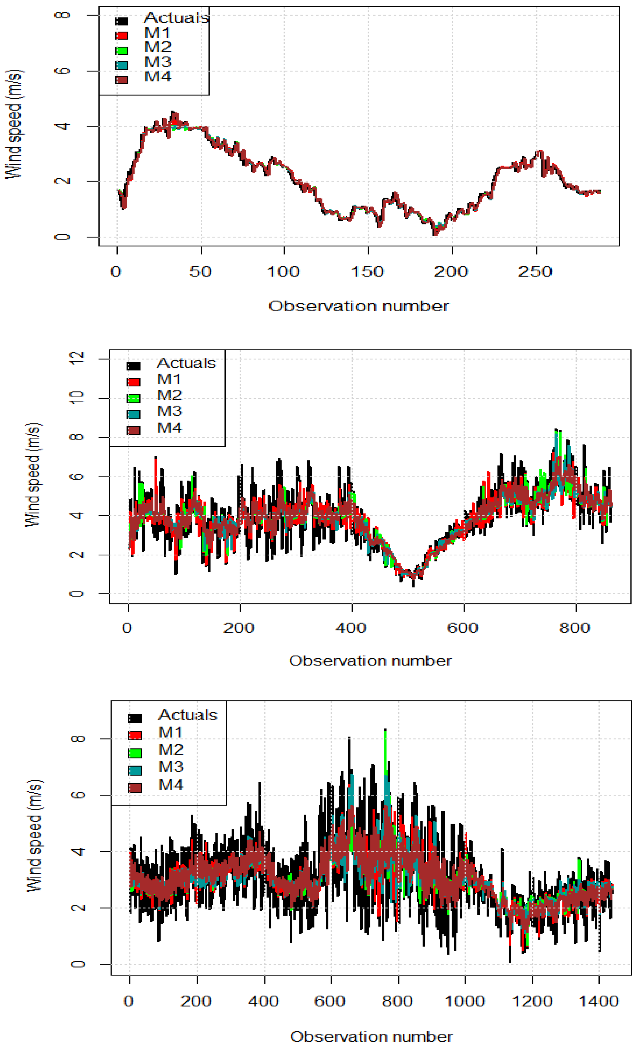
  • The practicability and efficacy of the proposed forecasting model were confirmed empirically via prediction metrics.
  • The study has been conducted in a way that is reliable and easy to replicate.
The study uses high-resolution minute-based granularity wind speed data measured by a R.M. Young (05103 or 03001) anemometer instrument. These data were downloaded (http://www.sauran.ac.za) (accessed on 15 December 2022) from Richtersveld (RVD), Central University of Technology (CUT), and University of Pretoria (UPR) radiometric stations in South Africa. The CUT station is located on the roof of a building at the CUT university, in the Free State province, at latitude −29.121337, longitude 26.215909, and an elevation of 1397 m. The RVD station is located in the desert region of the Northern Cape at latitude −28.56084061 and longitude 16.76145935, with an elevation of 141 m. The UPR station is located on the roof of a building at the University of Pretoria, in the Gauteng province, at latitude −25.75308037, longitude 28.22859001, and an elevation of 1410 m. We deliberately selected the stations to test how robust the proposed modelling and prediction approach would be under varying weather conditions. To our knowledge, a study of this type has not been conducted at these three Southern African Universities Radiometric Network (SAURAN) stations.

1.2. Overview of Related Studies

Several forecasting methods, including physical methods, statistical methods, hybrid models, and machine learning techniques, have been applied in an attempt to accurately forecast wind speed (see e.g., [5,10,11,19,20,21,22,23,24]). Although physical models (e.g., numerical weather prediction (NWP)) can effectively predict atmospheric dynamics, they have many limitations, including the use of a large amount of numerical weather data and the need for large computational time [2], which is costly and beyond the reach of a developing country such as South Africa. These methods are often reserved for medium- to long-term forecasting [7].
Statistical methods, on the other hand, make use of historical wind speed time series data to construct time series models, such as the linear autoregressive moving average (ARMA) model [2,4]. These models are generally reserved for capturing short-time phenomena [25,26,27,28]. For instance, ref. [15] presented an ARMA model to predict wind speed. The ARMA model was able to represent the actual features of wind speed. However, the ARMA model does not directly take into account changes in other related random variables or other exogenous variables. In essence, ARMA captures only a linear relationship, and it is generally suited to establishing a low-order time series model. To circumvent the nonstationarity inherent in the data, ARMA models have been extended to ARIMA models [29,30], seasonal ARIMA (SARIMA) models [31,32], and multiple linear regression coupled with SARIMA (SARIMAX) models, i.e., SARIMA models with exogenous variables [33].
Unlike statistical models, machine learning techniques are nonlinear approximators that can effectively capture nonlinear characteristics inherent in wind speed data that are impossible to capture using statistical methods. Hence, these techniques have gained popularity in wind speed forecasting [34]. Recent advances in machine learning algorithms have led to GBDTs becoming increasingly popular due to their quick training times, improved accuracy and flexibility, support for central processing units (CPU) (better than graphics processing units (GPU) used by ANNs), and ability to effectively handle large datasets [35,36,37,38,39,40,41,42]. Among the GBDTs, XGBoost, light gradient boosting machine (LGB), and stochastic gradient boosting machine (SGB) have been successfully applied in various fields, ranging from finance [36] to renewable energy [35,37,38,39,40,42]. For instance, ref. [38] employed the improved XGBoost to improve the accuracy of wind speed predictions. The authors compared the XGBoost with backpropagation neural networks (BPNN) and linear regression (LR) models and found that XGBoost has high predictive accuracy. In [40], the authors explored short-term wind speed forecasting using ANNs, SGBs, and generalised additive models (GAMs). The results showed that the SGB outperforms other models based on mean absolute error (MAE) and mean percentage error (MAPE). Overall, GBDTs have several advantages over other machine learning models: high efficiency in the prediction domain, the robustness of model tuning, improved prediction accuracy, and ease of interpretation [35,36,37,38,39,40,41] (also see Table 1).
Hybrid models combine more than one forecasting method to form a new one (see, e.g., [37,43,44,45]). Using different time-varying datasets, ref. [46] concluded that hybridisation ensures the accurate modelling of complex autocorrelation structures that are often inherent in time series data. As a result, hybrid methods have been proven to yield high prediction accuracy when handling time-series data with complex structures (see, e.g., [46]). For instance, to optimise the ARIMA model’s parameters, ref. [45] implemented an enhanced hybrid technique that combines an ARIMA and Kalman filter (KF) model via particle swarm optimisation (PSO). From the study results, the proposed approach improved the forecasting accuracy of the ARIMA model. In a similar study, ref. [37] proposed a new hybrid machine learning model that combines the LGB model and the Gaussian Process Regression (GPR) model to solve the probabilistic prediction problem of wind speed. In predicting wind speeds for a real wind farm in the United States, the proposed LGB-GPR model improved the point forecast accuracy and probabilistic forecast reliability when compared to individual SVR, LR, random forest (RF), GPR, ANN, long-term short memory (LSTM), and LGB.
To enhance the accuracy of the wind speed forecasting model, nonlinear, and nonstationary wind speed data must be pre-processed using an appropriate data decomposition technique. In recent years, WTs have gained some attention [18] in wind speed forecasting due to their excellent properties in both time and frequency domain time series analysis. Furthermore, WT is known to reveal patterns, discontinuities, and trends in time series by splitting them into low-frequency and high-frequency signals [47]. In essence, the WTs decompose original wind speed data to construct constitutive series that are statistically more sound (i.e., less variant) than the original, thereby reducing forecasting complexity [2,4,8,27]. For instance, ref. [25] proposed a repeated WT-ARIMA model (RWT-ARIMA). The RWT-ARIMA model was found to be more effective in improving the forecasting accuracy of the WT-ARIMA model in very short-term wind speed forecasting. In a similar study, ref. [44] combined WT, ARIMA, and machine learning algorithms (SVR and RF) in short-term wind speed forecasting using 10-min interval wind speed data. After fitting an ordinary ARIMA model to capture linear components, the residuals were decomposed using db3 level 5 WT and fed into the SVR or/and RF. Compared to the individual ARIMA model, the proposed strategy produced more accurate results. The authors of [43] proposed a hybrid model comprising WT, genetic algorithm (GA), and SVM in wind speed forecasting. A case study of a wind farm in North China demonstrated that this method provides more accurate and robust forecasts by fine-tuning the parameters in SVM using the GA to ensure generalisation. In contrast to the ARIMA model, GA and SVR are advantageous since they can avoid local optima, which is a deficiency of the ARIMA model [48,49,50,51,52] (also see Table 1). Despite the GA’s greater reliability, these techniques have a slower convergence rate than SVR algorithms.
Table 1. Summary of the strengths and weaknesses of the models employed in developing the WT-ARIMA-GBDTs-SVR model.
CategoryModelMeritDemeritReferences
StatisticalARIMAExcellent in handling linearity.Difficulty in capturing nonlinearity.[25,29,30,44,51,53]
Machine LearningSVRHigh convergence speed. Handles small data excellently.Inefficiency in handling large-scale dataset.[15,48,50,52,54]
Machine LearningXGBoostFaster and robust model tuning; highly scalable; flexible and versatile.Can overfit small datasets.[35,36,37,38,39,55]
Machine LearningLGBHigh training speed; Better accuracy; Support GPU learning; Capable of handling large-scale data.It produces more complex trees, and can overfit small datasets.[35,36,37,38,39]
Machine LearningSGBHighly predictive accuracy and flexibility.Can handle both categorical and numerical values.Require lots of trees and can overfit data. Can be computationally expensive.[40,41,42]
Signal processingWTExcellent features in the time and frequency domain. Can handle non-stationary data.Difficult to identify the most appropriate decomposition level.[56,57]

1.3. Suggested Modelling Approach

Wind speed is chaotically intermittent and is often characterised by inherent linear and nonlinear patterns as well as nonstationary behaviour; thus, it is generally difficult to predict it accurately and efficiently using a single linear or nonlinear model [25,46,53,54]. We suggest combining WT, ARIMA, and XGBoost via SVR to predict high-resolution short-term wind speeds.
In the literature, wavelet decomposition of a signal is followed by separate modelling of subseries using appropriate techniques. In the last step, sub-series predictions are reconciled (through summation) (see, e.g., [25]). In addition to its simplicity, this conventional approach (individual modelling and summation of subseries predictions) incorporates errors from each subseries into the final predictions. This compromises the accuracy and robustness of the final predictions. The authors of [25] discussed the difficulty in capturing high-frequency subseries when using the ARIMA model, which led to large errors when predicting using the WT-ARIMA model. High-frequency wind speed subseries (particularly at low levels) with nonlinear features adversely affect the accuracy and reliability of wind speed predictions from the ARIMA model. In this case, the uncertainty and inaccuracy of wind power predictions will result in energy costs rising, as additional reserves are required to maintain energy balance and ensure optimal unit commitment. Furthermore, ref. [58] also showed that wind turbine energy costs associated with forecast errors can reach 10% of total wind energy turnover.
Although the RWT-ARIMA model was found to reduce error accumulation to some extent, these techniques require more computational time than highly efficient machine learning algorithms such as the XGBoost and RF (see, e.g., [
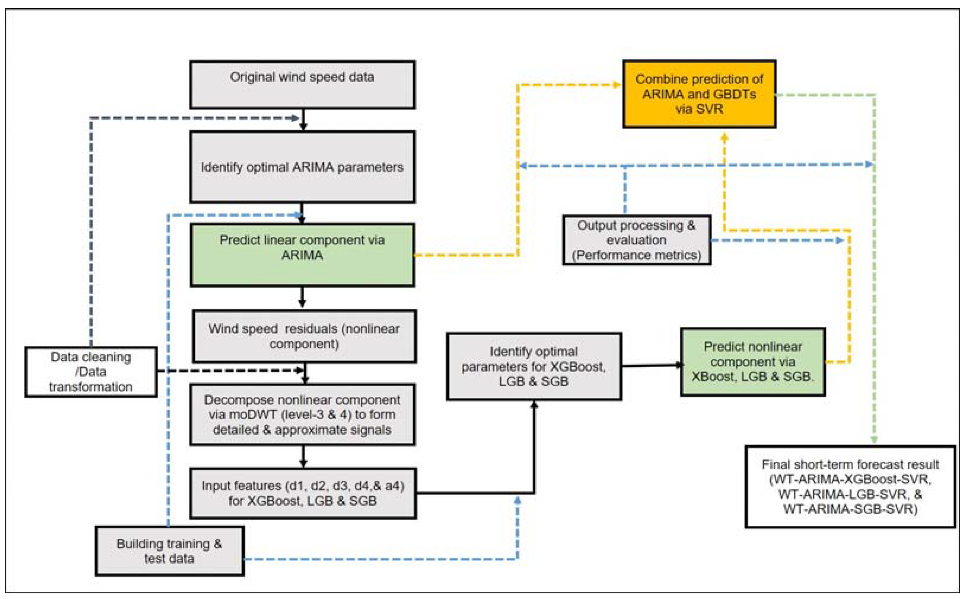
59]). Hence, this study proposes a new novel hybrid model, namely WT-ARIMA-XGBoost-SVR to circumvent error accumulation in the final wind speed predictions. In essence, the proposed strategy leverages the advantages of WT (excellent at denoising high variant signals), ARIMA (captures linearity very well), GBDTs (high accuracy, robust model tuning, highly scalable, sparse with computational efficiency), and SVR algorithms (high convergence speed with small sample sizes) to predict short-term wind speed with high precision and efficiency. In the aforementioned hybrid modelling strategy, the ARIMA model is employed to capture the linear component infused in the original wind speed data. The resultant residuals (i.e., nonlinear component) from fitting the ARIMA model are disaggregated into several less noisy subseries by WT. As input features, these subseries are fed into an XGBoost model to capture the nonlinear component that could not be captured by an ARIMA model. The final predicted value is determined by combining the predicted values from the ARIMA model and XGBoost using SVR. The efficacy of the proposed WT-ARIMA-XGBoost-SVR in short-term wind speed prediction is evaluated against the WT-ARIMA-LGB-SVR and WT-ARIMA-SGB-SVR. Although recent advances in computing power have led to more advanced and accurate machine-learning algorithms, ARIMA is still one of the most widely used models for wind speed short-term forecasting and benchmarking. For instance, in [60], the ARIMA model outcompeted Gated Recurrent Unit (GRU) and LSTM algorithms in short-term wind speed forecasting. Therefore, both the point and interval predictions of the proposed approach are also benchmarked against the ARIMA model to better evaluate its efficacy.
Overall, the current study will contribute to the existing renewable energy literature in the following ways: (a) In an effort to enhance short-term wind speed prediction accuracy, boosting and vector machine learning techniques are introduced; (b) High efficient and robust gradient decision trees are used instead of the classical ARIMA models, which are prone to struggling with nonlinearity and large datasets; (c) The effect of each subseries prediction error on overall wind speed prediction is minimised by utilising all wavelet decomposed subseries as input features into the XGBoost; (d) To some extent, the developed hybrid approach accurately, and efficiently captures nonlinear components associated with wind speed turbulence and gusts; (e) The proposed model is applied on different datasets from different locations as well as terrain complexity and used for forecasting over different time spans within the short-term forecasting framework to assess its robustness.

1.4. Structure of the Paper

The rest of the paper is structured as follows. Theory and fundamentals are given in Section 2, followed by the materials and methods presented in Section 3. Discussion of the results and conclusions are given in Section 4 and Section 5, respectively.

2. Theory and Fundamentals

2.1. Wavelet Transform

Using the WT, insightful and meaningful information can be collected, while noise and irregular patterns are removed from the time series data. WT is superior to Fourier transforms (which can only handle stationary data with fixed windows), as it can handle nonstationary data and use different time resolutions for varying frequencies [4,18,22,27,56,57]. In essence, WT decomposes the signal into different scale components with statistically more sound properties. By modelling these components separately, the accuracy of the model can be improved.
There are two main wavelet transform categories, namely the continuous wavelet transform (CWT) and discrete wavelet transform (DWT). The CWT, which is the addition of all time signal, multiplied and shifted versions of the mother wavelet
ψ ( a , b ) = 1 | a | ψ t b a ,
denoted by [22,56,57]:
CWT y ( a , b ) = 1 | a | + y t ψ t b a d t
where y t is the signal to be analysed, ψ a , b t * represents the conjugate of the mother wavelet ( ψ a , b t ) scaled by a factor a > 0 and time-shifted by parameter b. Each scale corresponds to the width of the wavelet. The DWT differs from CWT in that the mother wavelet scaling factor a = 2 i and the shifting (translation) factor b = 2 j are discrete such that DWT decomposition is given by [22,56,57]:
DWT y ( a , b ) = 1 | 2 i | + y t ψ t k 2 j 2 i d t
The DWT of level m = l o g int N of the wind speed data y t of a sample of size N is determined by passing y t through filter functions, resulting in the approximation coefficient vector a m and detail coefficient vector d m .
y t = a m ( t ) + j = 1 m d j ( t )

2.2. Autoregressive Integrated Moving Average Models

ARMA models are parametric models for stationary univariate time series and were discovered and popularised by [29]. In addition to their simplicity and robustness, ARMA models are advantageous in forecasting, as they capture the linear component excellently [25,29,30,44,51,53,54]. Hence, these are the most popular forecasting approaches.
ARMAs offer a parsimonious definition of a stationary method based on the auto-regression AR (p) of order p and moving average MA (q). For stationary time series, the ARMA model combines AR (p) and MA (q) such that [29,30]:
ARMA ( p , q ) : y t = c + i = 1 p φ i y t i + i = 1 q θ i e t i + e t
where yt is a stochastic process, c is a constant, and e t N (0, σ 2 ). In practice, time series is usually nonstationary. To achieve stationarity in the time series, regular (nonseasonal) differencing of order d, a positive integer excluding zero, is effected. Thus, the ARMA model can accommodate a nonstationary time series by differencing it d times resulting in the ARIMA (p, d, q) model. The ARIMA (p, d, q) can be mathematically expressed as follows [29]:
φ p ( B ) ( 1 B ) d y t = c + θ q ( B ) e t ,
where
φ p ( B ) = 1 B φ 1 B 2 φ 2 B p φ p ,
θ q ( B ) = 1 B θ 1 B 2 θ 2 B q θ q ,
and B is the backward shift operators. According to [29], modelling using the ARIMA model is a three-step process, namely (a) model identification, (b) parameter estimation, and (c) diagnostic checking. Model identification (step (a)) generally involves the utilisation of Box-cox transformation and differencing to achieve stationary of the time series, and the use of autocorrelation (ACF) and partial autocorrelation (PACF) to determine the optimal order of AR and MA, as proposed by [29]. The Akaike Information Criterion (AIC) and Bayesian Information Criterion (BIC) are frequently employed to elect the best parameters (see, e.g., [30,61,62,63] for details).

2.3. Support Vector Regression

In addition to having strong kernel tricks and solid mathematical theory, SVRs are nonlinear models that have a high convergence speed and can handle smaller data well [15,48,50,52,54]. As a matter of fact, the Gauss radial basis function utilised in this study exhibits high adaptability and high convergence areas in both low- and high-dimensional spaces [53] (also see Table 1).
Developed by [64], the SVR is based on the notion of risk structural minimisation, which minimises the upper limit of generalisation error as a function of the sum of training error and confidence [65]. Consider a training dataset denoted by
D = { ( x 1 , y 1 ) ,   ( x 2 , y 2 ) , ,   ( x n , y n ) } ,
then the regression formula can be expressed as
f x = ω i ϕ i x i + b ,   ϕ i :   R n F ,   ω i F , b R ,   for   i = 1 , n
where ω i are the weights (or support vector) estimated from the training data, b is the threshold value, and ϕ i are nonlinear mapping functions which map the sample datasets to high-dimensional feature space F [52]. Based on the structural risk minimisation principle, the weights ω i can be obtained from the sample data by minimising the following quadratic programming problem [48,52,64,65]:
min ω , a , ξ , ξ 1 2 | | ω | | 2 + C i = 1 n ( ξ i + ξ i )
such that
y i ω i . ϕ i ( x i ) b | ε + ξ i , ξ i , ξ i 0 , i = 1 , 2 , , n
where . denote a Euclidean norm, a constant C is the cost coefficient, also called the penalty factor, is greater than zero, and it controls the empirical risk degree of the SVR model. The features are denoted by n, whilst the ξ i , ξ i * 0 are the slack variables or the relaxation factors [65]. ξ ε (⋅) is the ε-intensive loss function and is defined as follows:
ξ ε   y i = 0 , if y i f x i ε , f x i y i ε , otherwise .
By solving the optimisation problem, the estimation function can be obtained as follows:
f ( x ) = i = 1 n ( α i α i ) K ( x i , x j ) + b
subject to α i   0 , α i * C , i = 1 n α i * α i = 0 , and K x i , x j is the kernel function. In this study, a kernel based on the Gaussian function, which is used to overcome the nonlinear regression problem, is given by the equation below:
K ( x i , x j ) = e x p ( γ | | x i x j | | 2 )
The cost (C) and gamma ( γ = 1 2 σ 2 ) are optimisation parameters that control the empirical risk level of the SVR model and the width of the kernel function, respectively.

2.4. Gradient Boosting Decision Tree Algorithms

As sequential ensemble techniques, GBDTs use information from previously developed weak classifiers to improve the model [35,36,37,38,39]. The process is repeated several times until an accurate model is constructed [35,36,37,38,39]. The result is achieved by dividing the training data, using each part to train different models, and finally combining the results [36].

2.4.1. Extreme Gradient Boosting Machine

XGBoost models are highly accurate, scalable, faster, and versatile gradient boosting techniques that support parallel computing, estimate tree matching, effectively handle sparse data, and improve CPU [35,36,39,55]. XGBoost (built on CPU devices just like LGBs) is developed by applying greedy algorithms to the objective function; continuously building decision trees leads to a complete model [35,55]. This algorithm can be viewed as an additive model that contains M decision trees given by the following equation [55]:
Y i = m = 1 M f m ( x i ) ,   f m F ,
where fm and F denote a decision tree and the function of the decision trees, respectively. This robust algorithm has faster model tuning and training, as it employs a regularisation technique. This is the same regularisation described by the following objective function [35,55], which also enables XGBoost to control overfitting [35].
L ( θ ) = i = 1 n ( L ( Y i . y i ) ) + m = 1 M φ ( f m ) , θ = ( f 1 , f 2 , , f m ) ,
where L denotes the loss function and φ the regularisation function, is given by [35,55]:
φ ( f ) = α | f | + 0.5 β | | w | | 2
where f denotes the number of branches; α and β represents the penalty factors; and is w a vector denoting the value of each leaf. XGBoost uses a stepwise forward algorithm to simplify model complexity [35,55]. Every time the model adds a decision tree, it learns a new function and its coefficients to match the residuals predicted in the last step [55]. The learning rate, maximum tree depth, and minimum child weight are the important parameters that control overfitting in the XGBoost algorithm.

2.4.2. Light Gradient Boosting Machine

The LGB is a type of GBDT that utilises a novel gradient-based one-sided sampling (GOSS) technique that downsamples the instances on the basis of gradients [35,36]. This technology allows the LGB model to work faster (than XGBoost [35]) while maintaining a high level of accuracy. Furthermore, LGB is different from other GBDTs in that it grows decision tree leaf by leaf instead of checking all previous leaves for each new leaf [35,36,37]. This technique, which is designed to improve the implementation time (of other GBDTs such as the XGBoost) and lower memory usage, also supports CPU learning, and is very efficient when handling large-scale data [35,36,37]. Suppose that there is a dataset V = { ( x 1 , y 1 ), ( x 2 , y 2 ), …, ( x N , y N )}, such that x i R n , x R , and N are the number of samples, then an LGB model can be described by the following equation [37]:
f M ( x ) = m = 1 M V ( x ; ε m ) ,
where V x ; ε m denotes a single binary regression tree, ε m is the parameter of the tree, and M is the number of the trees. In the LGB model, the final prediction result is obtained by fusing (linearly) the prediction results of several decision trees [37,55]. Since this algorithm can easily overfit small datasets [35,36,37,55], setting a maximum number of tree depth parameters is essential to address this drawback [37].

2.4.3. Stochastic Gradient Boosting

SGBs are machine learning algorithms created by building a series of shallow and weak trees that each learns and improves from its predecessors [40,41,42]. Stage-wise fitting is used with this technique. In spite of the SGB’s high flexibility and prediction accuracy, this algorithm can easily overfit the training dataset [40,41,42]. The SGB model is given by the following equation:
f ( x ) = m = 1 M β m b ( x ; γ m ) ,
where b x ; γ m R are functions of x characterised by the expansion parameters β m and γ m which are fitted in a stage-wise to delay over-fitting the model. Hence, when fitting SGB, the following parameters are critical to ensure optimal performance of the model: Number of trees: This is the total number of trees that need to be adjusted or fitted by the algorithm. Overfitting can occur if the number of trees is set too high; Interaction depth: This is the number of splits in each tree, and it controls the difficulty of the boosted ensemble; and Learning rate: In gradient descent algorithms, shrinkage controls the speed of descent. When values are smaller, overfitting is reduced, but it also takes longer to find the most appropriate fit.

3. Materials and Methods

3.1. Proposed Approach

The combinations of various models, such as wavelets and machine learning, are known as hybrid models. The rationale behind hybrid modelling is to improve overall forecast accuracy by retaining the advantages of each technique. The contribution of each model to the proposed WT-ARIMA-XGBoost-SVR model is described as follows:
  • The ARIMA was chosen as it is excellent at capturing linear components when forecasting wind speed on a short-term horizon. Furthermore, the ARIMA model is simple to use, flexible, and can detect trends and patterns in time series.
  • In addition to being a time-frequency domain technique, WT is preferred for the decomposition of wind speed residuals since it is efficient and can effectively handle nonstationary fluctuations. The WT also enhances the predictive ability of models, as it presents high-frequency resolution at low frequencies and high time resolution at high frequencies such that noise is removed and patterns or trends are revealed.
  • To circumvent ARIMA’s deficiency in capturing the nonlinearity (such as wind turbulence) component inherent in wind speed data, a highly accurate, scalable, fast, versatile, and flexible nonlinear XGBoost is used to predict the decomposed nonlinear wind speed residuals.
  • In addition to its high convergence speed, a nonlinear SVR model is preferred for prediction combination over a linear combination method (such as direct summation), as it considers nonlinear structure when combining predictions, thereby minimising error accumulation.
An alternative approach would be to substitute the ARIMA part for neural network autoregression (NNAR), which is more efficient and less sensitive to stationarity and nonlinearity. The XGBoost could be replaced by a more robust but less efficient LSTM. However, the study scope is limited to the proposed approach, whose process is shown in Figure 1. Algorithm 1 lays out the detailed steps for the process shown in Figure 1.
Algorithm 1. WT-ARIMA-GBDTs-SVR
INPUT: Wind speed time series data Y t
A.
Data cleaning
1.
The original wind speed data from three datasets of interest are cleaned to handle anomalies, such as invalidities and missing data, that might occur due to environmental factors or instability of the data collection system. We treat all observed wind speeds greater than 15 m/s as outliers (and are removed). Over 15 m/s, the wind turbine’s blades spin rapidly, which might cause the turbine to break down; thus, its operation is usually restricted. In some instances, wind turbines are switched off when the velocity exceeds 22 m/s, which is also referred to as feathering.
B.
Data partition
2.
Each dataset is divided into two sets, namely the training set (80%) and the testing set (20%).
3.
In the proposed strategy, the training set is utilised to build the model, while the testing set validates each of the established models.
C.
Train and predict using the ARIMA model
4.
Determine ARIMA orders using the “auto.arima” function in the R program using the training dataset.
5.
Predict wind speed data to capture (predict) linear components using the optimal ARIMA model such that the predictions are denoted by Y ^ τ .
6.
Generate the ARIMA residuals using the entire wind speed dataset such that residuals are calculated by R y t = Y t Y ^ ε with Y ^ ε being the fitted values.
7.
Validate the efficacy of ARIMA predictions based on root mean square error (RMSE) and MAE.
D.
Data decomposition
8.
The ARIMA residuals (or nonlinear components) are decomposed into less noisy subseries using level 3 and 4 maximal overlap DWT (MODWT).
9.
Divide decomposed subseries ( R y t ) into training set (80%) ( R t r a i n ) and testing set (20%) ( R t e s t )
E.
Train and predict using the XGBoost model
10.
Using a grid search, determine model hyperparameters such as the interaction depth, learning rate, maximum number of trees, and minimum child using the training dataset ( R t r a i n ) of the decomposed subseries as input features. The objective is to obtain those parameters that minimise the RMSE and MAE.
11.
To capture the nonlinear component, the testing set ( R t e s t ) of the decomposed subseries is utilised as input features into the optimal XGBoost model for prediction.
12.
The efficacy of the predictions ( R ^ t e s t ) from the XGBoost model is validated using the decomposed subseries based on RMSE and MAE.
F.
Combination of predictions via SVR
13.
Use a grid search to identify hyperparameters, such as the Cost and Gamma, before the SVR is utilised to combine sub-series predictions.
14.
To arrive at the final prediction, the ARIMA and XGBoost predictions are combined through the SVR algorithm to form the WT-ARIMA-XGBoost model such that
Y ^ f i n a l = S V R r b f ( Y t T , Y ^ τ T , R ^ t e s t )
G.
Final prediction evaluation
15.
The efficacy of the final predictions is validated using error metrics (MAE, MAPE, R2, and RMSE) and prediction interval indices (PINAD and PINAW) against the original wind speed testing dataset.
OUTPUT: Predictions Y ^ f i n a l performance metrics (MAE, MAPE, RMSE, and R2), prediction interval indices (PINAD and PINAW).

3.2. Case Study Description

In this study, univariate time series of wind speed data were analysed from three radiometric stations in South Africa, namely the CUT, the RVD, and the UPR. Table 2 is a description of these three stations.
These minutely averaged wind speed data were collected from SAURAN (https://sauran.ac.za/) (accessed on 15 December 2022) and their details are provided in Table 3 (also see Figure 2). The three stations are equipped with an R.M. Young (05103 or 03001) anemometer that measures wind speed accurately. All measurements are conducted at sub-6 s intervals using South African Standard Time (SAST) [66]. There were two sampling sets per station: a training set and a testing set, with an 80%:20% split. To assess the forecasting performance of the proposed methodologies, locations with varying meteorological patterns are chosen over days, months, and years.

3.3. Computational Tools

The models described in the previous section were trained and tested on an Intel Core i5 processor running in the HP notebook development environment (R package 4.2.2). The best-fit ARIMA model was developed through the “forecast” library. The library “waveslim”, through the function “modwt”, decomposes the three wind speed datasets. To tune the SVM models, the “svm” functions of the “e1071” library are used. XGBoost and SGB were implemented through the libraries “xgboost” and “gbm”, respectively. The LGB was fitted using “lightgbm”.

3.4. Prediction Evaluation Metrics

3.4.1. Point Prediction Evaluation Metrics

The forecasting performance of all fitted models is assessed and compared using the MAE (in m/s), RMSE (in m/s), and MAPE (%). Smaller values of these performance metrics imply a better model [67]. Suppose that yt and y t ^ are the actual and predicted wind speed values at time t, respectively. The error terms are denoted by e t = y t y t ^ , where t = 1 , , m . Then, the forecasting accuracy measures are given by the following expressions:
M A E = 1 m t = 1 m | e t | ,
R M S E = 1 m t = 1 m e t 2 ,
M A P E = 1 m t = 1 m | e t | × 100 .
MAE and RMSE are based on absolute errors and are scale-dependent [30,63,67]. These are the most widely used error indicators. MAE indicator changes are linear and intuitive. Due to the square of the error value, the RMSE penalises larger errors more than smaller ones. The MAPE indicator is often used to compare predictive performance between two datasets [30]. Similar to the RMSE, the normalised MAPE indicator is highly sensitive to distribution bias and skewness. Additionally, MAPE imposes a heftier penalty on minus errors rather than on positive errors [30,68].
The coefficient of determination R 2 0 , 1 is also employed to examine the predictive strength of the fitted models (see [68] for details). The coefficient of determination determines the linear correlation between the actual data and the predictive model. The closer the values of R 2 to 1, the better the prediction model:
R 2 = 1 t = 1 m ( y ^ t y t ) 2 t = 1 m ( y ¯ t y t ) 2 ,
where y t and y ¯ t respectively represent the actual and mean wind speed value. The R 2 metric is preferred for model selection as compared to the aforementioned metrics. However, larger model deviance can affect the performance of this indicator [68].

3.4.2. Residual Analysis

Summary statistics and boxplots of residuals denoted by e t j = y t j y ^ t j for each of the models, M j ,   j = 1 , , k , are used to evaluate the over and under predictions of each model. Negative residuals ( e t j < 0 ) imply over-predictions, whereas positive residuals ( e t j > 0 ) imply under-predictions.

3.5. Prediction Interval Evaluation Metrics

3.5.1. Prediction Interval Width

The prediction interval (PI) represents a wide range of possible probabilistic values within which the actual values of the wind speed should lie with a certain specified probability. In general, the lower and upper boundaries cover the unidentified target value of the future value with any probability 1 β % referred to as confidence level. When dealing with the uncertainty associated with point forecasts, it is essential to provide forecast intervals to cater for uncertainties [69]. The prediction interval width (PIW) denoted by P I W t , t = 1 , , m ; is given by:
PIW t = UL t LL t
where UL t denotes the upper limit, whilst LL t is the lower limit of the prediction interval.

3.5.2. Prediction Interval Indices

A PI with nominal confidence (PINC) with 1 β 100 % is defined as the probability that the forecasted y ^ t LL t , U L t and is calculated as follows:
PINC = ( y t ( UL t , LL t ) = ( 1 β ) 100 % )
In this study, we employ two well-known PI indices, namely the prediction interval normalised average deviation (PINAD) and prediction interval normalised average width (PINAW) [69]. These PI performance measures are respectively represented by the following mathematical equations [69]:
P I N A D = 1 m R i = 1 m Z t ,
Z t = LL t y t ,   y t < LL t , 0 ,   y t LL t , UL t ,   y t UL t , y t UL t ,  
and
PINAW = 1 m R t = 1 m ( UL t LL t ) ,
where U L t and LL t are the upper and lower limits of the PI, respectively. R = range ( y t ) is the variation in the range of the actual wind speed values. It is preferable to have a lower PINAD value, as it indicates less deviation from the target value. Smaller PINAW values are also preferred since they resemble narrower PIs. However, PIs are often computationally expensive, as they require long training times and are sensitive to deviations from normality [30,68]. Furthermore, the PI size increases with an increase in the forecast horizon length [30,68].

4. Empirical Results

4.1. Exploratory Data Analysis

Table 4 summarises the descriptive statistics for wind speed measurements at the three radiometric stations of interest. All three datasets are platykurtosis (kurtosis less than 3). However, the RVD dataset is peakier than the other two datasets (CUT and UPR). Furthermore, UPR has the least variation whilst RVD exhibits the most variation.

4.2. Empirical Results and Discussion

4.2.1. Model Parameter Settings

A stepwise searching approach (grid search) was used to select the optimal hyperparameters for the regression models. The resultant optimal intervals of important parameters are presented in Table 5. We adjusted the model hyperparameters with changes in the prediction horizon to try to improve the model’s performance.
The computational time for each model on the training and testing datasets is presented in Table 6. The WT-ARIMA-LGB-SVR is the most efficient, followed by the WT-ARIMA-XGBoost-SVR and ARIMA models. The WT-ARIMA-SGB-SVR produced the least (but reasonable) computational time among all models.

4.2.2. Wavelet Transform

The three residual wind speed datasets were decomposed into detailed signals and one approximation signal using a level 3 (for RVD) and level 4 MODWT (for CUT and UPR), as shown in Figure 3. The three datasets show an increase in variation as decomposition levels decrease.
Table 7 compares the point prediction results for the four models fitted to the RVD, CUT, and UPR data. In this paper, M1, M2, M3, and M4 refer to WT-ARIMA-XGBoost-SVR, WT-ARIMA-LGB-SVR, WT-ARIMA-SGB-SVR, and ARIMA. The metric values for the best model are bolded in Table 7. For all three datasets, model M1 outperformed all other models in terms of RMSE, MAPE, MAE, and R2. Except for M1, model M2 demonstrated superiority for CUT and UPR datasets, followed by M3 and M4 across all performance indicators. Based on RMSE and MAE for RVD data, model M4 performed second compared to model M1. For the same dataset, model M2 outperformed model M3 based on RMSE. Model performance is higher for smaller datasets and lesser for larger datasets. Additionally, as the prediction horizon lengthens, the prediction task becomes more challenging. The performance of each model varies with the dataset size, locations, terrain complexity, and forecasting time spans. Furthermore, the prediction task becomes more complex as the prediction horizon increases. Overall, model M1 (followed by M2) provides better prediction performance for the three wind speed datasets (see also Figure 4).

4.2.3. Percentage Improvement

The percentage improvement in prediction accuracy between M1 and the other three models is presented in Table 8. Model M1 reduced RMSE by 3.2% for RVD data, 9.8% for CUT data, and 3.6% for UPR data. For RVD and CUT datasets, M1 reduced MAE by 2.3% and 20.3%, respectively, while MAE for UPR data was reduced by 5.6%. In terms of MAPE, model M1 reduced MAPE by an average of 3.3% for RVD, 20.9% for CUT, and 5.2% for UPR. The highest average improvement for the R2 indicator was observed for UPR (10.3%), followed by CUT (9.1%) and RVD (0.2%) data. Across all performance indices, it can be observed that M1 improves M4 the most, followed by M3 for larger datasets (CUT and UPR). This implies that M2 has the second-best predictive strength behind M1 for CUT and UPR. Furthermore, the least improved model for RVD data is M4, followed by M2, based on RMSE, MAE, and R2. Although all models are hyrestetic (see Figure 4), the proposed M1 provides a better and more reliable improvement when compared to the other three models. Furthermore, there still exists some lag in the predicted values when wind speed irrupts, particularly for CUT and UPR (largest) data.

4.2.4. Residual Analysis

Table 9 summarises the residuals for the fitted models for RVD, CUT, and UPR datasets. The best models’ values are bolded. Except for M4, residuals for all models are positively skewed for all three datasets, indicating frequent small losses (underestimation) with fewer chances of extreme gains (overestimation). For RVD, residuals for model M4 are more or less normally distributed (skewness = −0.020). As anticipated, the ARIMA model seems to fit the smaller dataset very well at a shorter prediction horizon. Kurtosis tests for all datasets and models indicate positive values of less than 3. Thus, the distributions are mesokurtic compared to the normal distribution. All models have light-tailed residuals with minimal outliers. The low variation within observations suggests that the data are highly concentrated around the mean as well (also see Figure 5). Overall, M1 predicts RVD, CUT, and UPR data with the highest accuracy than any other model.

4.2.5. Evaluation of Probabilistic Predictions

Table 10 compares model performance based on 90% PI indices, PINAW and PINAD. The values of the best model are shown in bold. PINAD values were the smallest for CUT and UPR data using models M1 and M3, respectively, and the smallest for RVD data using model M3. The narrowest PINAW was achieved by M1 for CUT and UPR data, followed by M4 for the same datasets. PINAW was the narrowest for RVD data for model M4, followed by models M2, M3, and M3. For all three datasets, M1 produced the fewest values outside the 90% prediction interval. In general, model M1 quantifies CUT and UPR data more reliably and with less uncertainty than any other model.

5. Conclusions

With consideration of linear and nonlinear components (volatility and noise) infused in wind speed data, this paper presents a comparison of hybrid strategies to short-term wind speed predictions using a combination of wavelet transforms (WT), autoregressive moving averages (ARIMA), gradient boosting decision trees (GBDTs), and support vector regression (SVR). Thus, the study compared the predictive performance and robustness of the WT-ARIMA-XGBoost-SVR against the WT-ARIMA-LGB-SVR, WT-ARIMA-SGB-SVR, and benchmark ARIMA using minutely averaged wind speed data from the RVD, CUT, and UPR radiometric stations located in South Africa.
In summary, the following conclusions could be reached from the comparative analysis: (a) The wavelet decomposition of the highly variable and nonlinear components of the wind speed data reduced noise and volatility, thereby improving the prediction performance of all three hybrid strategies; (b) The ARIMA was successfully implemented in all three datasets to capture the linear component of wind speed, while the GBDTs captured the complex nonlinear component; (c) Both XGBoost and LGB successfully saved computational time and improved the prediction performance of the WT-ARIMA-XGBoost-SVR and WT-ARIMA-LGB-SVR, respectively. Furthermore, LGB was more efficient (required less training time), followed by XGBoost, and ARIMA. Similar results were found in [35,36,37,39,40]; (d) The RBF kernel SVR effectively reconciled ARIMA and GBDT predictions with faster convergent speed for RVD and CUT than for large samples (UPR). These results are consistent with those in [15,48,50,52]; (e) Based on RMSE, MAE, MAPE, and R2 a comparative study of point predictions showed that WT-ARIMA-XGBoost-SVR is the most suitable model for predicting all three datasets; (f) For shorter prediction intervals (288 min), ARIMA has the second best performance (WT-ARIMA-XGBoost-SVR), while for longer intervals (1440 min), it has the poorest performance. These results concur with those in [25,26,27,28,35,36,37,38,39]. In general, all models’ performance declines with increased prediction horizons. Compared to the other three models, the proposed WT-ARIMA-XGBoost model has less sensitivity to terrain changes and a prediction horizon; (f) The WT-ARIMA-XGBoost model significantly outperformed all other models in residual analysis, achieving the least standard deviation (i.e., spread) across all datasets. Thus, this model predicts the three wind speed data with the highest accuracy than any other model; and (g) Based on PINAWs, all three datasets can be quantified more reliably with less uncertainty through the WT-ARIMA-XGBoost-SVR model than through any other model.
From the overall comparative analysis, we can conclude that the WT-ARIMA-XGBoost-SVR model overcomes the individual models’ inherent limitations and achieves better accuracy, efficiency, robustness, and reliability across all datasets. These results (which are consistent with some studies reviewed in the literature, such as [38,55]) can be used by utility managers and policymakers to develop effective grid management strategies for integrating large volumes of wind power into their electric grids. Furthermore, the findings can be applied to effectively manage wind power voltage fluctuations and ensure power system dispatch safety.
Despite its ability to predict wind speed over short prediction horizons on different terrains (with varying climatic conditions) within South Africa, the proposed approach displays some gaps when wind speed changes abruptly. It will be interesting to see how high-variant and large wind speed datasets (outside South Africa) will affect model accuracy and robustness. This is our future research problem.

Author Contributions

Conceptualisation, K.S.S.; methodology, K.S.S.; software, K.S.S.; validation, K.S.S.; formal analysis, K.S.S.; investigation, K.S.S.; resources, K.S.S. and E.R.; data curation, K.S.S.; writing—original draft preparation, K.S.S.; writing—review and editing, K.S.S. and E.R.; visualisation, K.S.S.; supervision, E.R. All authors have read and agreed to the published version of the manuscript.

Funding

This research received no external funding.

Institutional Review Board Statement

Not applicable.

Informed Consent Statement

Not applicable.

Data Availability Statement

These wind speed data can be downloaded from SAURAN (http://www.sauran.ac.za) (accessed on 15 December 2022).

Acknowledgments

Not applicable.

Conflicts of Interest

The corresponding author states that there is no conflict of interest.

Abbreviations

ACFAutocorrelation Function
AICAkaike Information Criterion
ARIMAAutoregressive Integrated Moving Average
ARMAAutoregressive Moving Average
BICBayesian Information Criterion
CWTContinuous Wavelet Transform
DWTDiscrete Wavelet Transform
GAGenetic Algorithm
GBDTGradient Boosted Decision Trees
KFKalman Filter
LGBLight Gradient Boosting Machine
MAEMean Absolute Error
MODWTMaximal Overlap Discrete Wavelet Transform
PACFPartial Autocorrelation Function
PIPrediction Interval
PIWPrediction Interval Width
PINCPrediction Interval with Nominal Confidence
PINADPrediction Interval Normalised Average Deviation
PINAWPrediction Interval Normalised Average Width
PSOParticle Swarm Optimisation
RMSERoot Mean Square Error
SAURANSouthern African Universities Radiometric Network
SGBStochastic Gradient Boosting Machine
SVRSupport Vector Regression
WTWavelet Transform
XGBoostExtreme Gradient Boosting Machine

References

  1. Chaturvedi, D.K.; Isha, I. Solar Power Forecasting: A Review. Int. J. Comput. Appl. 2016, 145, 28–50. [Google Scholar] [CrossRef]
  2. Chen, N.; Qian, Z.; Meng, X. Multistep Wind Speed Forecasting Based on Wavelet and Gaussian Processes. Math. Probl. Eng. 2013, 2013, 461983. [Google Scholar] [CrossRef]
  3. Zhang, J.; Wei, Y.; Tan, Z.F.; Ke, W.; Tian, W. A Hybrid Method for Short-Term Wind Speed Forecasting. Sustainability 2017, 9, 596. [Google Scholar] [CrossRef]
  4. Berrezzek, F.; Khelil, K.; Bouadjila, T. Efficient wind speed forecasting using discrete wavelet transform and artificial neural networks. Rev. Artif. 2019, 33, 447–452. [Google Scholar] [CrossRef]
  5. Qian, Z.; Pei, Y.; Zareipour, H.; Chen, N. A review and discussion of decomposition-based hybrid models for wind energy forecasting applications. Appl. Energy 2019, 235, 939–953. [Google Scholar] [CrossRef]
  6. Sohoni, V.; Gupta, S.; Nema, R. A Critical Review on Wind Turbine Power Curve Modelling Techniques and Their Applications in Wind Based Energy Systems. J. Energy 2016, 2016, 8519785. [Google Scholar] [CrossRef]
  7. Hanifi, S.; Liu, X.; Lin, Z.; Lotfian, S. A Critical Review of Wind Power Forecasting Methods-Past, Present and Future. Energies 2020, 13, 3764. [Google Scholar] [CrossRef]
  8. Singh, P.K.; Singh, N.; Negi, R. Short-Term Wind Power Forecasting using Wavelet-based Hybrid Recurrent Dynamic Neural Networks. Int. J. Perform. Eng. 2019, 15, 1772–1782. [Google Scholar] [CrossRef]
  9. Zhang, Y.; Yang, S.; Guo, Z.; Guo, Y.; Zhao, J. Wind speed forecasting based on wavelet decomposition and wavelet neural networks optimized by the Cuckoo search algorithm. Atmos. Ocean. Sci. Lett. 2019, 12, 107–115. [Google Scholar] [CrossRef]
  10. Soman, S.S.; Zareipour, H.; Malik, O.; Mandal, P. A review of wind power and wind speed forecasting methods with different time horizons. N. Am. Power Symp. 2010, 2010, 1–8. [Google Scholar] [CrossRef]
  11. Wang, X.C.; Guo, P.; Huang, X.B. A review of wind power forecasting models. Energy Procedia 2011, 12, 770–778. [Google Scholar] [CrossRef]
  12. Rae, G.; Erfort, G. Offshore wind energy—South Africa’s untapped resource. J. Energy S. Afr. 2020, 31, 26–42. [Google Scholar] [CrossRef]
  13. Liu, H.; Tian, H.Q.; Li, Y.F. Comparison of two new ARIMA-ANN and ARIMA-Kalman hybrid methods for wind speed prediction. Appl. Energy 2012, 98, 415–424. [Google Scholar] [CrossRef]
  14. Zhang, W.; Qu, Z.; Zhang, K.; Mao, W.; Ma, Y.; Fan, X. A combined model based on CEEMDAN and modified flower pollination algorithm for wind speed forecasting. Energy Convers. Manag. 2017, 136, 439–451. Available online: https://api.semanticscholar.org/CorpusID:113862762 (accessed on 19 September 2023). [CrossRef]
  15. Zhang, Y.; Zhao, Y.; Kong, C.; Chen, B. A new prediction method based on VMD-PRBF-ARMA-E model considering wind speed characteristic. Energy Convers. Manag. 2020, 203, 112254. Available online: https://www.osti.gov/servlets/purl/1114086 (accessed on 11 March 2023). [CrossRef]
  16. Shi, X.; Lei, X.; Huang, Q.; Huang, S.; Ren, K.; Hu, Y. Hourly Day-Ahead Wind Power Prediction Using the Hybrid Model of Variational Model Decomposition and Long Short-Term Memory. Energies 2018, 11, 3227. [Google Scholar] [CrossRef]
  17. Valdivia-Bautista, S.M.; Domínguez-Navarro, J.A.; Pérez-Cisneros, M.; Vega-Gómez, C.J.; Castillo-Téllez, B. Artificial Intelligence in Wind Speed Forecasting: A Review. Energies 2023, 16, 2457. [Google Scholar] [CrossRef]
  18. Kisi, O.; Shiri, J.; Makarynskyy, O. Wind speed prediction by using different wavelet conjunction models. Int. J. Ocean. Clim. Syst. 2011, 2, 189–208. [Google Scholar] [CrossRef]
  19. Dhiman, H.S.; Anand, P.; Deb, D. Wavelet transform and variants of SVR with application in wind forecasting. In Innovations in Infrastructure; Deb, D., Balas, V., Dey, R., Eds.; Springer: Singapore, 2019; pp. 501–511. [Google Scholar] [CrossRef]
  20. Liu, H.; Tian, H.; Liang, X.; Li, Y. New wind speed forecasting approaches using fast ensemble empirical model decomposition, genetic algorithm, Mind Evolutionary Algorithm and Artificial Neural Networks. Renew. Energy 2015, 8, 1066–1075. [Google Scholar] [CrossRef]
  21. Ma, L.; Luan, S.; Jiang, C.; Liu, H.; Zhang, Y. A review on the forecasting of wind speed and generated power. Renew. Sustain. Energy Rev. 2009, 13, 915–920. [Google Scholar] [CrossRef]
  22. Wang, J. A Hybrid Wavelet Transform Based Short-Term Wind Speed Forecasting Approach. Sci. World J. 2014, 2014, 914127. [Google Scholar] [CrossRef]
  23. Xie, H.; Ding, M.; Chen, L.; An, J.; Chen, Z.; Wu, M. Short-term wind power prediction by using empirical mode decomposition based GA-SYR. In Proceedings of the 2017 36th Chinese Control Conference (CCC), Dalian, China, 26–28 July 2017; pp. 1934–1978. [Google Scholar] [CrossRef]
  24. Zhao, J.; Li, X.; Hao, J.; Lu, J. Reactive power control of wind farm made up with doubly fed induction generators in distribution system. Electr. Power Syst. Res. 2010, 80, 698–706. [Google Scholar] [CrossRef]
  25. Aasim; Singh, S.N.; Abheejeet, M. Repeated wavelet transform based ARIMA Model for very shortterm wind speed forecasting. Renew. Energy 2019, 136, 758–768. [Google Scholar] [CrossRef]
  26. Huang, C.J.; Kuo, P.H. A Short-Term Wind Speed Forecasting Model by Using Artificial Neural Networks with Stochastic Optimization for Renewable Energy Systems. Energies 2018, 11, 2777. [Google Scholar] [CrossRef]
  27. Saroha, S.; Aggarwal, S. Wind power forecasting using wavelet transforms and neural networks with tapped delay. J. Power Energy Syst. 2018, 4, 197–209. [Google Scholar] [CrossRef]
  28. Wang, H.Z.; Lei, Z.X.; Zhang, X.; Zhou, B.; Peng, J.C. A review of deep learning for renewable energy forecasting. Energy Convers. Manag. 2019, 198, 111799. [Google Scholar] [CrossRef]
  29. Box, G.E.P.; Jenkins, G.M. Time Series Analysis: Forecasting and Control; Holden-Day: San Francisco, CA, USA, 1976. [Google Scholar]
  30. Hyndman, R.J.; Athanasopoulos, G. Forecasting Principles and Practice, 2nd ed.; OTexts: Melbourne, Australia, 2021. [Google Scholar]
  31. Tyass, I.; Bellat, A.; Raihani, A.; Mansouri, K.; Khalili, T. Wind Speed Prediction Based on Seasonal ARIMA model. E3S Web Conf. 2022, 336, 00034. [Google Scholar] [CrossRef]
  32. Elkashaty, O.A.; Daoud, A.A.; Elaraby, E.E. Forecasting of Short-Term and Long-Term Wind Speed of Ras Gharib Using Time Series Analysis. Int. J. Renew. Energy Res. 2023, 13, 258–272. [Google Scholar] [CrossRef]
  33. Ahn, E.J.; Hur, J. A short-term forecasting of wind power outputs using the enhanced wavelet transform and arimax techniques. Renew. Energy 2023, 212, 394–402. [Google Scholar] [CrossRef]
  34. Xie, A.; Yang, H.; Chen, J.; Sheng, L.; Zhang, Q. A Short-Term Wind Speed Forecasting Model Based on a Multi-Variable Long Short-Term Memory Network. Atmosphere 2021, 12, 651. [Google Scholar] [CrossRef]
  35. Ke, G.; Meng, Q.; Finley, T.; Wang, T.; Chen, W.; Ma, W.; Liu, T.Y. Lightgbm: A highly efficient gradient boosting decision tree. In Proceedings of the Advances in Neural Information Processing Systems 30: Annual Conference on Neural Information Processing Systems, Long Beach, CA, USA, 4–9 December 2017; pp. 3146–3154. [Google Scholar]
  36. Daoud, E.A.L. Comparison between XGBoost, LightGBM and CatBoost Using a Home Credit Dataset. Int. Sch. Sci. Res. Innov. 2019, 13, 6–10. [Google Scholar] [CrossRef]
  37. Liu, G.; Wang, C.; Qin, H.; Fu, J.; Shen, Q. A Novel Hybrid Machine Learning Model for Wind Speed Probabilistic Forecasting. Energies 2022, 15, 6942. [Google Scholar] [CrossRef]
  38. Cai, R.; Xie, S.; Wang, B.; Yang, R.; Xu, D.; He, Y. Wind Speed Forecasting Based on Extreme Gradient Boosting. IEEE Access 2020, 8, 175063–175069. [Google Scholar] [CrossRef]
  39. Chen, T.; Guestrin, C. XGBoost: A scalable tree boosting system: A scalable tree boosting system. In Proceedings of the 22nd Acm Sigkdd International Conference on Knowledge Discovery and Data Mining, San Francisco, CA, USA, 13 August 2016; pp. 785–794. [Google Scholar] [CrossRef]
  40. Daniel, L.O.; Sigauke, C.; Chibaya, C.; Mbuvha, R. Short-Term Wind Speed Forecasting Using Statistical and Machine Learning Methods. Algorithms 2020, 13, 132. [Google Scholar] [CrossRef]
  41. Friedman, J.H. Stochastic gradient boosting. Comput. Stat. Data Anal. 2019, 38, 367–378. [Google Scholar] [CrossRef]
  42. Singh, U.; Rizwan, M.; Alaraj, M.; Alsaidan, I. A Machine Learning-Based Gradient Boosting Regression Approach for Wind Power Production Forecasting: A Step towards Smart Grid Environments. Energies 2021, 14, 5196. [Google Scholar] [CrossRef]
  43. Liu, D.; Niu, D.; Wang, H.; Fan, L. Short-term wind speed forecasting using wavelet transform and support vector machines optimized by genetic algorithm. Renew. Energy 2014, 62, 592–597. [Google Scholar] [CrossRef]
  44. Patel, Y.; Deb, D. Machine Intelligent Hybrid Methods Based on Kalman Filter and Wavelet Transform for Short-Term Wind Speed Prediction. Wind 2022, 2, 37–50. [Google Scholar] [CrossRef]
  45. Su, Z.; Wang, J.; Lu, H.; Zhao, G. A new hybrid model optimized by an intelligent optimization algorithm for wind speed forecasting. Energy Convers. Manag. 2014, 85, 443–452. [Google Scholar] [CrossRef]
  46. Zhang, G.P. Time series forecasting using a hybrid ARIMA and neural network model. Neurocomputing 2003, 50, 159–175. [Google Scholar] [CrossRef]
  47. Adamowski, K.; Prokoph, A.; Adamowski, J. Development of a new method of wavelet aided trend detection and estimation. Hydrol. Process. 2009, 23, 2686–2696. [Google Scholar] [CrossRef]
  48. Chen, J.; Xue, X.; Ha, M.; Yu, D.; Ma, L. Support Vector Regression Method for Wind Speed Prediction Incorporating Probability Prior Knowledge. Math. Probl. Eng. 2014, 2014, 410489. [Google Scholar] [CrossRef]
  49. Farsi, M.; Doreswamy, H.; Manjunatha, B.R.; Gad, I.; Atlam, E.; Althobaiti, A.; Elmarhomy, G.; Elmarhoumy, M.; Ghoneim, O.A. Parallel genetic algorithms for optimizing the SARIMA model for better forecasting of the NCDC weather data. Alex. Eng. J. 2020, 60, 1299–1316. [Google Scholar] [CrossRef]
  50. Quan, J.; Shang, L. An Ensemble Model of Wind Speed Forecasting Based on Variational Mode Decomposition and Bare-Bones Fireworks Algorithm. Math. Probl. Eng. 2021, 2021, 6632390. [Google Scholar] [CrossRef]
  51. Scrucca, L. On Some Extensions to GA Package: Hybrid Optimisation, Parallelisation and Islands Evolution. R J. 2017, 9, 187. [Google Scholar] [CrossRef]
  52. Yang, Z.J. Kernel-based support vector machines. Comput. Eng. Appl. 2008, 44, 1–6. [Google Scholar]
  53. Chen, N.; Sun, H.; Zhang, Q.; Li, S. A Short-Term Wind Speed Forecasting Model Based on EMD/CEEMD and ARIMA-SVM Algorithms. Appl. Sci. 2022, 12, 6085. [Google Scholar] [CrossRef]
  54. Jiang, P.; Wang, B.; Li, H.; Lu, H. Modeling for chaotic time series based on linear and nonlinear framework: Application to wind speed forecasting. Energy 2019, 173, 468–482. [Google Scholar] [CrossRef]
  55. Zheng, H.; Wu, Y. A XGBoost Model with Weather Similarity Analysis and Feature Engineering for Short-Term Wind Power Forecasting. Appl. Sci. 2019, 9, 3019. [Google Scholar] [CrossRef]
  56. Addison, P.S. The Illustrated Wavelet Transform Handbook: Introductory Theory and Applications in Science, Engineering, Medicine, and Finance; Institute of Physics Pub: Bristol, UK, 2002. [Google Scholar]
  57. Goswami, J.C.; Chan, A.K. Fundamentals of Wavelets: Theory, Algorithms and Applications; John Wiley and Sons: New York, NY, USA, 1999. [Google Scholar]
  58. Fabbri, A.; Roman, T.G.S.; Abbad, J.R.; Quezada, V.H.M. Assessment of the cost associated with wind generation prediction errors in a liberalized electricity market. IEEE Trans. Power Syst. 2005, 20, 1440–1446. [Google Scholar] [CrossRef]
  59. Spiliotis, E.; Abolghasemi, M.; Hyndman, R.J.; Petropoulos, F.; Assimakopoulos, V. Hierarchical forecast reconciliation with machine learning. Appl. Soft Comput. 2021, 112, 107756. [Google Scholar] [CrossRef]
  60. Liu, X.; Lin, Z.; Feng, Z. Short-term offshore wind speed forecast by seasonal ARIMA—A comparison against GRU and LSTM. Energy 2021, 227, 120492. [Google Scholar] [CrossRef]
  61. Ong, C.S.; Huang, J.J.; Tzeng, G. Model identification of ARIMA family using genetic algorithm. Appl. Math. Comput. 2005, 164, 885–912. [Google Scholar] [CrossRef]
  62. Schwarz, G. Estimating the Dimension of a Model. Ann. Stat. 1978, 6, 461–464. Available online: http://www.jstor.org/stable/2958889 (accessed on 4 April 2023). [CrossRef]
  63. Wei, W. Time Series Analysis: Univariate and Multivariate Methods, 2nd ed.; Pearson Addison Wesley: Boston, MA, USA, 2006. [Google Scholar]
  64. Vapnik, V.N. The Nature of Statistical Learning Theory; Springer: New York, NY, USA, 1995. [Google Scholar]
  65. Zhang, B.; Yang, T.; Hong, H.; Cheng, G.; Yang, H.; Wang, T.; Cao, D. Research on Long Short-Term Decision-Making System for Excavator Market Demand Forecasting Based on Improved Support Vector Machine. Appl. Sci. 2021, 11, 6367. [Google Scholar] [CrossRef]
  66. Brooks, M.J.; Du Clou, S.; Van Niekerk, W.L.; Gauché, P.; Leonard, C.; Mouzouris, W.J.; Meyer, R.; Van der Westhuizen, N.; Van Dyk, E.E.; Vorster, F.J. SAURAN: A new resource for solar radiometric data in Southern Africa. J. Energy S. Afr. 2015, 26, 2–10. Available online: http://www.scielo.org.za/scielo.php?script=sci_arttext&pid=S1021-447X2015000100001&lng=en&tlng=en (accessed on 19 September 2023). [CrossRef]
  67. Zhang, J.; Hodge, B.S.; Florita, A.R.; Lu, S.; Hamann, H.F.; Banunarayanan, V. Metrics for Evaluating the Accuracy of Solar Power Forecasting. In Proceedings of the 3rd International Workshop on Integration of Solar Power into Power Systems, London, UK, 21–22 October 2013. [Google Scholar]
  68. Gensler, A. Wind Power Ensemble Forecasting: Performance Measures and Ensemble Architectures for Deterministic and Probabilistic Forecasts. Ph.D. Thesis, University of Kussel, Kassel, Hessen, Germany, 21 September 2018. [Google Scholar]
  69. Quan, H.; Srinivasan, D.; Khosravi, A. Uncertainty handling using neural network-based prediction intervals for electrical load forecasting. Energy 2014, 73, 916–925. [Google Scholar] [CrossRef]
Figure 1. The WT-ARIMA-GBDTs-SVR strategy for short-term wind speed prediction.
Wind 04 00003 g001
Figure 2. Minute wind speed data for RVD (top left panel), CUT (top right panel), and UPR (bottom centre panel).
Wind 04 00003 g002
Figure 3. MODWT results for minutely averaged wind speed data for RVD (top left panel), CUT (top right panel), and UPR (bottom centre panel).
Wind 04 00003 g003
Figure 4. Comparison of predicted wind speeds and actual wind speed data for RVD (top panel), CUT (middle panel), and UPR (bottom panel) datasets.
Wind 04 00003 g004
Figure 5. Boxplots of the residuals for RVD (top left panel), CUT (top right panel), and UPR (bottom centre panel).
Wind 04 00003 g005
Table 2. Location coordinates of the stations.
StationLongitudeLatitudeAltitude (m)Topography
RVD−28.5608406116.76145935141Inside enclosure in desert region
CUT−29.12133726.2159091397Roof of a building
UPR−25.7530803728.228590011410Roof of a building
Table 3. Details of sampled data division.
StationNumber of DaysMonthSample SizeTraining SetTesting Set
RVD17 September 201914401152288
CUT315–19 August 201943203456864
UPR51–5 June 2021720057601440
Table 4. Descriptive statistics for wind speed data (m/s).
StationRVDCUTUPR
Min0.03600
Q13.3821.5881.063
Mean7.1252.7702.229
St. Dev.3.6031.6511.488
Q310.0303.8193.154
Max14.4009.13010.790
Skewness−0.2180.4790.646
Kurtosis−1.055−0.0660.368
Table 5. Model hyperparameter optimisation interval.
ModelHyperparameterOptimisation Interval
ARIMAAutoregressive term0–3
Moving average term0–3
Integrated term0–1
WTwf
n.levels
boundary
‘la8’
3–4
‘periodic’
SVRRBF kernel: Cost1–50
RBF kernel: Gamma0.5–10
XGBooostMax Tree depth3–15
Learning rate0.05–0.95
Min child1
LGBMax Tree depth3–15
Learning rate0.05–1
SGBInteraction depth3–7
Learning rate0.005–0.3
Number of trees6–59
Table 6. Implementation time (in seconds) for the fitted models on the wind speed data.
ModelTraining and Testing Dataset (s)
ARIMA~7–15
WT-ARIMA-XGBooost-SVR~4–11
WT-ARIMA-LGB-SVR~3–9
WT-ARIMA-SGB-SVR~7–30
Table 7. Comparative analysis using error metrics.
IndicatorM1M2M3M4
RVD
RMSE (m/s)0.1740.1800.1810.179
MAE (m/s)0.1320.1350.1350.134
MAPE (%)8.68.88.89.2
R20.9760.9740.9740.974
CUT
RMSE (m/s)0.8130.8710.8940.912
MAE (m/s)0.5490.6240.6590.697
MAPE (%)14.416.717.418.3
R20.6930.6480.6280.613
UPR
RMSE (m/s)0.9340.9580.9680.979
MAE (m/s)0.6940.7200.7270.752
MAPE (%)23.124.024.424.7
R20.4160.3860.3730.359
Bold = Best model.
Table 8. Percentage improvement rates (%).
IndicatorM1:M2M1:M3M1:M4Mean
RVD
RMSE3.33.72.53.2
MAE2.52.71.72.3
MAPE1.41.56.93.3
R2−0.2−0.2−0.1−0.2
CUT
RMSE7.11012.29.8
MAE13.720.126.920.3
MAPE15.820.426.620.9
R2−6.5−9.4−11.5−9.1
UPR
RMSE2.53.64.83.6
MAE3.74.88.45.6
MAPE3.75.26.65.2
R2−7.1−10.3−13.6−10.3
Table 9. Comparison of models’ residuals (m/s).
StatisticM1M2M3M4
RVD
Std.Dev0.1750.1800.1810.179
Skewness0.1560.2390.273−0.020
Kurtosis1.5101.5241.5561.498
CUT
Std.Dev0.8120.8700.8940.912
Skewness0.3020.3150.2920.236
Kurtosis1.9391.0810.9250.594
UPR
Std.Dev0.9340.9570.9680.980
Skewness0.3080.3530.3440.197
Kurtosis1.0150.7320.9070.574
Bold = Best model.
Table 10. Comparative analysis of models using PI indices.
IndicatorM1M2M3M4
RVD
PINAW (%)12.46412.49613.20812.355
PINAD (%)0.2030.2290.1970.215
OL (count)27292830
OL (%)9.410.19.710.4
CUT
PINAW (%)33.79036.53537.37336.468
PINAD (%)0.6160.5500.5220.569
OL (count)84898684
OL (%)9.910.510.29.9
UPR
PINAW (%)37.24538.16638.70738.105
PINAD (%)0.5170.4990.5160.486
OL (count)143142142145
OL (%)9.99.99.910.1
OL = Number of predictions outside limits. Bold = Best model.
Disclaimer/Publisher’s Note: The statements, opinions and data contained in all publications are solely those of the individual author(s) and contributor(s) and not of MDPI and/or the editor(s). MDPI and/or the editor(s) disclaim responsibility for any injury to people or property resulting from any ideas, methods, instructions or products referred to in the content.

