1. Introduction
In recent years, renewable energy has exhibited exponential growth, contributing close to a considerable portion of global electricity production. Examples of these resources include hydroelectric, solar, biomass, geothermal, and wind energy. For instance, hydropower plants are the primary source of renewable electricity in Brazil, representing 56.66% of the electrical matrix [
1]. However, changes in rainfall patterns and severe El Niño/La Niña Southern Oscillation (ENSO) episodes can disrupt electricity availability, as evidenced by the water crisis between 2014 and 2015, triggered by an abnormal rainy season characterized by below-average precipitation and record high-temperature extremes [
2]. Also, thermoelectric plants are usually used in Brazil to regulate the system and meet the energy demand. However, due to the climate change crisis, several efforts have been made to reduce dependence on hydrothermal systems, such as increasing the electrical matrix’s diversification and their installed capacity. These efforts are now accompanied by concerns regarding the price fluctuations of oil derivatives and the difficulty of accessing natural gas, a significant portion of which is imported. These challenges are further compounded by logistical difficulties in transportation and distribution.
In this context, wind, solar, and biomass energies have emerged as convenient options. As reported in 2022, over the previous six years, solar and wind energy were the ones that sparked the greatest competition. This increased investment has the potential to significantly influence the cost of electricity bills. Also, the auction results confirm that Brazil has become a lucrative market for these industries, which continue to grow. In just five years, wind farms have more than doubled energy generation in the country, while solar plants have grown by over 25,000% [
3]. According to the 2023 National Energy Balance (BEN), wind, solar, and biomass energy now account for approximately 12%, 5%, and 8% respectively, of the Brazilian electrical matrix [
4].
Despite the availability of resources, the effectiveness of wind generation energy is still affected by its intermittent nature, which means there is typically a mismatch between generated energy and the load demand. Thus, this intermittency poses a significant obstacle within the wind power industry as it requires energy grid operators to continually align energy production with demand, regardless of the fluctuating production of wind energy [
5]. In addition, power storage is not easy, and the efficiency of batteries is another field of study. Given those challenges, the capacity to precisely predict wind speeds several time steps ahead for a specific location becomes a critical tool. It allows the managers of transmission services to strategize and plan their operations ahead of time, thereby optimizing the efficiency of the power grid [
6].
Moreover, the Brazilian National Electricity System Operator (ONS, Operador Nacional do Sistema Elétrico), responsible for managing, coordinating, and controlling the operations of electricity generation and transmission facilities, determines the hourly dispatch and energy prices with a time horizon of up to one week and a time discretization of up to half-an-hour [
7]. Therefore, improved wind power forecasting is essential to make the electricity system more reliable and to reduce grid operational costs.
The field of short-term wind power forecasting with error correction approaches has seen significant advancements recently, as highlighted in several key studies. Hybrid methodologies for wind power prediction based on error correction techniques have been developed with success in different geographic regions and climates. The application of deep learning algorithms, including Long-Short Term Memory (LSTM), Gated Recurrent Units (GRUs), and Recurrent Neural Networks (RNNs), brings important improvements to a predictive system for wind power values [
8]. However, one of the main challenges in this field is the availability of high-quality historical data for training these sophisticated models, especially in regions with limited monitoring infrastructure. Moreover, the computational resources required for deep learning algorithms can be substantial, limiting their practicality in some applications.
Comprehensive analyses of statistical and machine learning approaches for error correction in wind power prediction, focusing on short-term forecasts up to 6 h ahead and introducing a benchmarking framework, have been conducted [
9]. Despite the progress, a key limitation is the inherent uncertainty in short-term weather patterns, which can lead to challenges in achieving high prediction accuracy. Additionally, model generalization across different geographic locations and climates remains a challenge, as local factors can significantly impact wind behavior. An error correction model for wind prediction in Brazilian regions was implemented, showcasing superior performance compared to traditional statistical methods [
10]. However, the limited spatiotemporal availability of high-quality wind data in certain Brazilian regions remains a significant limitation. Additionally, the model’s performance may be influenced by the specific characteristics of the regions it was trained on, limiting its applicability to other areas.
An error correction study using machine learning models was developed with significant improvements of prediction errors by 20% and extending short-term forecasts to 12 h [
11]. Nevertheless, the accuracy of short-term wind power forecasts is still subject to the inherent variability of wind patterns, making it challenging to eliminate all prediction errors. Furthermore, the computational complexity of machine learning models can hinder their real-time implementation in operational forecasting systems. A comprehensive hybrid wind energy prediction system with preprocessing using wavelet techniques, Bayesian optimization, and a decomposition-segment error correction technique was developed [
12]. While these techniques offer promising results, they may require a significant amount of computational resources and expertise to implement effectively, which can be a limitation for some organizations with limited resources.
An advanced wind power prediction model combining outlier correction, ensemble reinforcement learning, and residual correction was proposed, outperforming traditional ensemble methods [
13]. However, the practical implementation of such advanced models can be challenging, and they may require substantial computational resources and data to train effectively. Moreover, the interpretation of model outputs and the incorporation of model uncertainty into decision-making processes remain important challenges.
Precise wind speed forecasting for wind energy development was addressed, introducing a two-stage decomposition ensemble interval prediction model that provided both point and interval predictions [
14]. However, achieving precise interval predictions is inherently challenging due to the complex and dynamic nature of wind behavior. Additionally, the availability of data with accurate wind speed measurements for model validation can be limited, which affects the model’s reliability. Data analysis of a wind turbine SCADA dataset in Turkey was conducted, emphasizing data quality and different preprocessing techniques [
15]. Nonetheless, data quality issues, such as missing or noisy data, can pose significant challenges in real-world wind energy projects. Preprocessing and data cleaning efforts may require substantial manual intervention, adding complexity and time to the analysis process.
A hybrid wind speed prediction model based on ARMA-SVR and error compensation was presented, demonstrating superior results [
16]. However, the performance of such models can be sensitive to the choice of hyperparameters and the specific characteristics of the data, making them less straightforward to apply universally. Additionally, they may require ongoing calibration to maintain accuracy. A short-term wind power prediction model employing LSTM and multiple error correction techniques was proposed, significantly improving prediction accuracy [
17]. Nevertheless, the availability of high-quality training data for LSTM models, as well as the computational resources needed for their training and deployment, can be limiting factors. Model interpretability can also be a challenge with complex deep learning models
In [
18] is proposed an efficient k-Nearest Neighbors (KNN) wind power prediction model that leverages multi-tupled meteorological input data. Their best results demonstrated that the KNN model with 4-tupled input outperforms the persistence method, achieving a root mean square error (RMSE) of 2.475%, mean absolute percentage error (MAPE) of 1.158%, and mean absolute error (MAE) of 15.839 kW. In contrast, the persistence method yields higher errors with an NRMSE of 17.809%, MAPE of 31.230%, and MAE of 204.5498 kW. The findings highlighted the effectiveness of the KNN model in accurately predicting wind power and reducing uncertainty. The study emphasizes the importance of selecting appropriate input tuples and demonstrates the potential of the KNN-based approach for optimizing wind energy systems.
The authors of [
19] introduced an approach that combines self-organized maps, radial basis function networks, and fuzzy logic to optimize the Numerical Weather Predictions (NWP). Their goal was to accurately estimate the power output of a wind plant over a 48-h horizon, in Denmark. The input data for the model consisted of wind speed measurements for the current and next hour. The normalized mean absolute error (NMAE) for the proposed system ranged between 5% and 14%, whereas the persistence model had an NMAE of 24%. Additionally, the normalized root mean square error (NRMSE) for the proposed system remained below 20%, while persistence reached 34%. Furthermore, their proposed model showed better performance compared to estimates based on the NWP and achieved results comparable to the best state-of-the-art models. These findings indicate that their proposed system provides improved accuracy, with lower errors and higher skill, making it a promising tool for wind power forecasting.
In the study [
20] the authors examined and compared the effectiveness of direct and iterative forecasting approaches for multi-step ahead wind speed prediction. They utilized multi-layer perceptron (MLP) and support vector machine (SVM) models to evaluate the performance difference between these mechanisms. The results demonstrated that the variation in performance depended on the prediction horizon and the specific models employed. Generally, direct forecasting exhibited a slight advantage regarding the RMSE and MAE, but occasionally performed worse in terms of the MAPE. The disparity between the mechanisms remained below 2% for all prediction horizons. However, there were instances where iterative forecasting, particularly with the SVM model, significantly outperformed direct forecasting. Overall, neither method consistently surpassed the other, emphasizing the importance of considering the specific context and characteristics of the model when selecting a forecasting mechanism. Every prediction model is prone to generating errors in their predictions. Recognizing this, researchers have conducted several studies that utilize the errors produced by these models to correct the initial output values.
As presented in [
21], an SVM and Extreme Learning Machine (ELM) were applied to predict the forecast error of a primary model. Both the persistence (Per) and SVM models were used as the primary model. This methodology was applied to both one-step and multi-step ahead predictions. The corrected wind power predictions are calculated based on the forecasted values from the primary model and the predicted error values. The final predictions are adjusted to ensure that they are within the permissible range of zero to the installed capacity of the wind farm. Different model combinations were assessed, including Per-SVM/Per-ELM and SVM-SVM/SVM-ELM, and found that they exhibited marginal differences among themselves. However, SVM proved more suitable as a forecast error model. For multi-step ahead predictions, the combination of SVM-ELM showed the highest prediction performance and the overall short-term wind power forecasting showed a general improvement when using the combined models.
Similarly, the reference [
22] proposed the introduction of a secondary model aimed at predicting the errors produced by a primary model which employs historical error values, wind power, and wind speed as predictors. The primary model utilizes NWP data, which is transformed by the wind power curve to optimize the correction model, and the authors conducted experiments using Boosted Trees, SVM, Neural Networks, and Random Forests to determine the most suitable parameters. Subsequently, the selected models were trained with the identified optimal parameters, and the outcomes were subjected to a comparative analysis. Notably, the Random Forest model exhibited the most promising results, demonstrating a substantial increase in precision compared to the other models. The enhancements observed were 98.05% for bias, 63.15% for the MAE, 54.87% for the RMSE, and 78.97% for the MSE.
Another study that aimed to correct a base model’s output was proposed in [
23], in which a second model utilized the information learned from the error mapping stage to correct the wind power predictions. By considering the implicit information contained in the prediction errors, the model aimed to reduce the inherent errors and improve the accuracy of the wind power forecasts. The short-term wind power forecasting method works in two stages. In the first stage, variational mode decomposition (VMD) is optimized using a flower pollination algorithm (FPA) to decompose the wind power sequence. Bi-directional long short-term memory (BiLSTM) neural networks are employed to capture time series features. The second stage involves principal component analysis (PCA) to reduce correlation among meteorological factors, followed by an error correction model based on BiLSTM. Experimental results demonstrate improved prediction accuracy compared to traditional methods for both single-step and multi-step ahead forecasting. This approach combines decomposition, feature extraction, and error correction to enhance wind power forecasting precision.
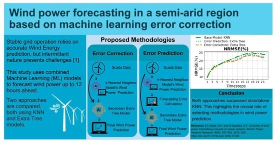
In this paper, we explore the potential of combined machine learning (ML) models for wind power forecasting up to 12 h ahead. We compare two distinct methodologies, error prediction, and error correction, each utilizing KNN as the primary model and Extra Tree as the secondary model. The methodologies vary based on the target for the second model and the flow of information, with the shared goal of improving the accuracy of predictions. Our main contribution is to evaluate these two techniques with Supervisory Control and Data Acquisition (SCADA) power data from a real wind farm operated inside one of the main Brazilian Northeast hotspots, with complex land surface and atmospheric local patterns. The findings will facilitate more efficient and reliable power generation in the region. The contributions of this paper are summarized as follows:
Introducing innovative error correction methods to enhance short-term wind power forecasting, potentially addressing machine learning model limitations in handling wind energy’s intermittent nature. Many studies often emphasizes the need for robust models in this context.
Focusing on a specific wind turbine SCADA dataset demonstrates practicality and addresses data availability challenges. It serves as a real-world data example. The Literature recognizes data quality challenges for training complex models, especially in regions with limited monitoring.
Innovative error correction methods aim to improve prediction accuracy up to 12 h ahead, addressing uncertainties in weather patterns and model generalization across diverse geographic locations. The existing literature acknowledges the inherent uncertainty in short-term weather patterns, impacting prediction accuracy.
Balancing computational complexity while extending short-term forecasts, offering insights into practicality. It can make advanced models more suitable for operational use. Studies notes that machine learning model complexity can hinder real-time implementation in operational forecasting.
Achieving significant prediction error reductions, though complete elimination remains challenging due to wind pattern variability. The existing literature presents various error correction techniques, but complete error elimination remains a challenge.
2. Materials and Methods
2.1. Study Area and SCADA Wind Power Data
In this paper, we looked at the Casa Nova II wind farm, operated by the Eletrobras CHESF, and installed in Casa Nova municipality, Bahia, Brazil (
Figure 1). This location has a Köppen classification defined as BSh, a semi-arid climate pattern, with hot and dry conditions all year. The wet season, which lasts from December to March, brings most of the annual rainfall, while the dry season lasts the rest of the year. This semi-arid climate puts Casa Nova at risk of drought during extended periods of low rainfall, leading to water scarcity concerns. The local vegetation and terrain have evolved to these conditions, including robust plant species suited to arid areas, such as the common Caatinga biome. Another important aspect of Casa Nova is its susceptibility to the local impact of the Sobradinho reservoir on its near-surface wind patterns and other meteorological dynamics [
24]. Functioning as an artificial lake designed for hydroelectric power generation under the auspices of Eletrobras CHESF, the Sobradinho reservoir contributes significantly to the region’s energy infrastructure. Eletrobras CHESF, recognized as one of Brazil’s prominent electricity providers with a capacity exceeding 10 GW, operates within the Northeastern region. Further insights can be found at their official website:
https://www.chesf.com.br/ (accessed on 12 July 2023).
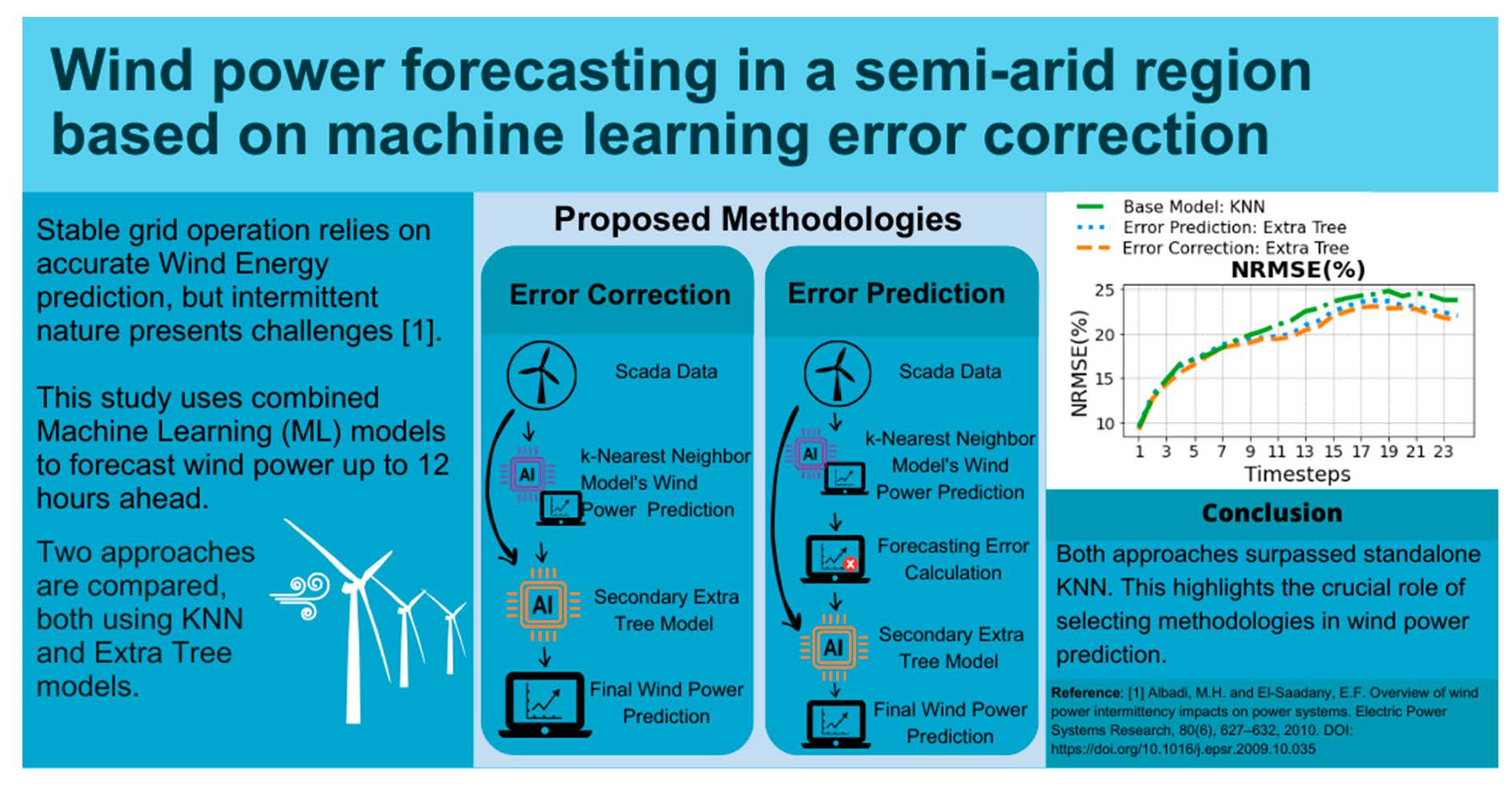
The dataset used in this work originates from a single Enercon E92 wind turbine’s SCADA system. With a 2350 kW rated power, this upwind turbine features a 92-m rotor diameter, resulting in a sizable 6648 m2 swept area. Its tower reaches a hub height of 98 m. Operational wind speeds range from a 2 m/s cut-in to a 25 m/s cut-off, with a rated wind speed of 13 m/s. Collected between 1 January 2020, and 30 April 2021, the dataset includes parameters recorded at 10-min intervals of wind speed, active power output, rotation, pitch, and yaw values. While pitch and yaw angles are presented in averaged values, the others encompass maximum, average, and minimum readings.
Wind speed (m/s) critically impacts power generation, improving turbine behavior predictions and power output estimates. It is a foundational feature in machine learning models, enabling the capture of wind-condition-to-power relationships. Our work focuses on forecasting active wind power (kW), leveraging real-time active power data to enhance short-term accuracy. Integration of this predictor empowers models to adapt swiftly to dynamic fluctuations. Additionally, pitch (degrees) influences turbine response, enhancing predictions during changing wind conditions. Incorporating pitch angle information refines forecasts under varying scenarios. Yaw (degrees), representing rotor misalignment, and rotation (RPM) are vital variables. Models considering yaw angles account for orientation effects, enhancing precision. Rotor speed inclusion captures dynamic rotational–power interactions, amplifying forecasting capabilities.
The wind power output data from the wind SCADA system were assessed according to the criteria applied by the Brazilian ONS and described in [
25], where a few adjustments were applied. In a nutshell, the wind power values were considered invalid under the following conditions: (1) negative values; (2) exceeding 10% of the turbine’s maximum nominal power, i.e., higher than 2585 kW; (3) frozen (unchanged) measurements during 1 h or more; (4) and finally, the last filter applied to the data series involves the elimination of data that includes days with less than 2.5 valid hours in the series. In this case, if a day does not have at least 2.5 h of valid data (fifteen values at 10-min intervals), the day is discarded. After the application of these filters, the removed values were not numerically filled.
Figure 2 illustrates the results of the quality control on the wind turbine’s power curve, while
Table 1 presents the statistical summary of the wind power values before and after the application of the quality filtering process, resulting in the removal of approximately 8% of the data. Within the wind power curve, a detailed examination revealed a significant portion of invalidated data points, notably characterized by negative values. Additionally, a distinct subset of data points exhibiting invalid characteristics was identified within intervals where power levels registered below 1000 kW. These discrepancies and anomalies in the data, if left unaddressed, could severely compromise the accuracy and reliability of subsequent analyses and predictions.
The authors in [
26] suggested that the invalidation of these intermediary data points could potentially be attributed to technical anomalies within the wind turbine itself or errors during the storage and transmission of information. Such technical discrepancies might arise due to sensor malfunctions, communication disruptions, or even system errors. Understanding the paramount significance of data quality in the realm of machine learning applications, the elimination of these outliers assumes pivotal importance. The process of identifying and removing these invalidated data points, or outliers, serves as a fundamental prelude to the subsequent implementation of machine learning forecasting models [
27]. By meticulously cleansing the dataset of these irregularities, the integrity of the data is upheld, paving the way for accurate and reliable training of machine learning models.
The recognition and removal of these outliers not only mitigate the potential introduction of misleading patterns but also foster the creation of robust and dependable predictive models. In the context of machine learning-based wind power forecasting, the meticulous curation of input data constitutes an essential step toward ensuring the validity and effectiveness of the models’ predictive outcomes. Therefore, the procedure of outlier elimination acts as a foundational measure to enhance the quality and utility of subsequent machine learning-based wind power forecasting endeavors.
Following the qualification procedures, a resampling step was performed to adjust the data to a 30-min frequency. Subsequently, a rigorous data cleaning process was executed, with a primary focus on the meticulous management of null or missing values. This process was undertaken to safeguard the integrity and reliability of the dataset, ensuring its suitability for subsequent analyses and modeling.
2.2. Machine Learning: Preprocessing and Forecasting Techniques
Meteorological variables are influenced by the time of day and season. They are usually represented by integers that typically range from 0 to 23 for hours and from 1 to 365 for days. However, the use of these values fails to account for the cyclical nature of time. For example, midnight (0 h) and 11 pm (23 h) are only an hour apart, but the numerical difference between their encodings is 23. In an ML context, hours that are temporally close should be represented with similar values to be accurately understood.
To address this issue, an alternative approach known as sine/cosine encoding or cyclic encoding was applied to capture daily and seasonal patterns in wind energy generation, and thus, provide a piece of important information for the predictive models. This method captures the periodic and gradual characteristics of time by combining the integer value with the periodicity of the trigonometric function, resulting in two variables derived from sine and cosine functions. This process essentially curls the time axis into a circle, connecting its start and end. The position of a time point on this circle is then represented by a pair of sine and cosine values, reflecting the cyclical nature of time. The equation for this technique is as follows [
28,
29]:
In which, is the integer value representing a particular time point of interest. The x-value corresponds to the horizontal direction on the X-axis, while the Y-axis represents the vertical direction, together establishing a rectangular coordinate system within the trigonometric circle. The variable n denotes the total number of hours in a day or the total number of days in a year, depending on the nature of the variable t. With the cosine-sine decomposition, a total of 16 features were obtained.
Both methods involved multi-step predictions, for that is necessary to construct a target that contains all of the information for the 24 time steps ahead. However, this approach led to data points being lost where there were missing data between the steps ahead. When data are missing, the current step can not be utilized, reducing the dataset from 23,328 to 17,190.
The performance of ML models is typically assessed by partitioning the data into distinct training and test sets. In this study, a dual-model methodology was employed. In the configuration of the initial model, an 80–20 split was implemented, that is 80% of the data (13,752 data points) were allocated for the training phase and the remaining 20% (3438 data points) were reserved for the testing phase. This split was designed to provide an ample volume of data for model training, while still reserving a significant subset for the unbiased evaluation of the model’s performance on unseen data. For the second model in the sequence, we further segmented the 20% holdout data from the original dataset. In this partitioning, 80% of the holdout data (2788 data points) were utilized for training and the remaining 20% (697 data points) were allocated for testing. By using this nested data splitting strategy, the two-model approach tested in our methodologies not only maintains data integrity and avoids overfitting but also validates the generalizability of the models on completely new, unseen data. Data normalization was also applied, calculated based on the training data, and later extended to the test data. This approach prevented contamination in the test set and mitigated variable dominance, ensuring a balanced and reliable analysis.
Two distinct approaches were explored in this study, both of which employed a two-step sequential modeling technique for predicting wind power (WP). The primary model across both methodologies is a KNN algorithm, which processes SCADA data to predict WP output across a horizon of 24 future time steps of 30 min, equivalent to a 12-h forecast window. The difference between the two approaches lies in the configuration and target assigned to a second model, that uses the Extra Trees Regressor algorithm. A more detailed description is exposed in the next section.
2.2.1. First Approach to ML Forecasting: Error Prediction
Systematic errors, which are typically responsible for consistent overestimation or underestimation in model predictions, are likely to affect all prediction models. However, the precision of these predictions can be improved by incorporating residual error values into the predicted series. This strategy helps to mitigate the negative effects of systematic errors, thereby enhancing the model’s overall accuracy to some extent [
30]. In this sense, for the first approach, the second model was introduced to estimate and correct the prediction error generated by the initial model, following the studies in [
21,
22]. A schematic representation of how the model receives the same SCADA data and the predicted output from the initial KNN model applied in this article was proposed by [
30]. The target of this model is the prediction error obtained from the first model. The error is calculated by Equation (
4). After receiving the output from the first model, the second model predicts the potential error. This predicted error is then summed up with the original output from the KNN model to adjust the forecasted WP. Mathematically, this correction process is represented by Equation (
5).
where,
is the wind power predicted by the KNN model,
is the actual observed wind power and
the error that the second model expects for the KNN model predictions. This methodology represents an innovative approach to correcting and fine-tuning predictive models by utilizing a second model to adjust the forecasted values based on anticipated errors.
2.2.2. Second Approach to ML Forecasting: Error Correction
The second approach also employs a two-model structure, in which the first model is the same KNN model used in the first methodology. However, the second model here uses the SCADA data and the KNN model’s output to directly predict the WP, instead of focusing on the predicted error. This approach, which corrects the prediction of WP, is represented by the flowchart shown in
Figure 3, and follows the proposed method in [
23]. The aim of the second methodology is to have a second model that learns from the initial model’s forecasts and SCADA data to predict the WP output. Essentially, the second model works as a fine-tuning layer to the KNN model’s output, which might result in an improved prediction. The corrected WP output in this methodology is the output from this second model. Hence, no explicit addition or correction operation is performed, unlike the first approach. This two-tiered approach combines the strengths of multiple models and provides a robust and adaptable system for predicting WP output based on the SCADA data. The effectiveness and performance of these methodologies were subsequently evaluated and compared using statistical metrics and time series comparison.
2.3. ML Performance Evaluation
The statistical metrics used in this study were traditional parameters such as the mean bias (MB), root mean square error (RMSE), normalized root mean squared error (NRMSE), and coefficient of correlation (R). These indices are recommended by various studies to assess the reliability and representativeness of the forecasting (e.g., Refs. [
18,
19,
21,
22,
23,
31]). The error metrics are defined in:
where
is the observed value;
is the predicted value at the time
i;
N is the number of tested samples; max
denotes the highest observed output class; and min
signifies the lowest observed output class. BIAS is defined as the mean error (MB) corresponding to the systematic error. The MB, NRMSE, and RMSE are error-based indices that quantify the deviations between the model predictions and the observed data. Smaller values of these indices indicate higher accuracy and better simulation quality. The RMSE stands out as an absolute measure of error, quantifying the magnitude of discrepancies between predictions and observations.
On the other hand, the NRMSE provides a relative perspective on the error. Due to its normalized nature, the NRMSE becomes especially useful when comparing errors across datasets of different scales or units. Considering the MB, this metric provides insight into the direction of the error. A positive bias indicates that the model, on average, overestimates the observations, while a negative bias suggests it underestimates them. Values of this index which are closer to zero indicate better alignment between predictions and observations, signifying superior simulation quality. On the other hand, the R serves as an indicator of linear association and agreement between the modeled and observed data. A value close to zero suggests a lack of correlation, while values closer to 1 or −1 indicate a strong positive or negative correlation between the two datasets.
To facilitate a quantitative analysis, a metric used by the authors in [
18,
21,
22] defines the degree of improvement of an advanced object concerning a reference object. This metric is also based on error evaluation, as illustrated below:
where
M represents the metric used for evaluation (e.g., the RMSE and NRMSE), and
denotes the improvement degree. When
is a positive value, it indicates that the advanced model outperforms the reference model, and vice versa. Here,
denotes the metric value obtained by a reference model, while
M represents the metric value being compared against the reference.
3. Results and Discussion
In this section, we divide our results into two parts. First, we present the main findings in a general analysis.This is followed by a detailed discussion and comparison with other studies related to wind power forecasting using ML methods, analyzing the performance of the two approaches explored in the present study.
Figure 4 presents the part of the results referred to at the 2nd, 6th, 12th and 24th wind power forecast time steps, between 15 and 29 of April. It only shows part of the test data Given that each time step represents 30 min, these correspond to 1, 3, 6, and 12 h ahead, respectively. It is noticed that the predictions utilizing solely the KNN model have greater difficulty in predicting peak values of the observed wind power values on more distant time steps (e.g., 6 and 12 h ahead). In the meantime, both the first and the second approaches demonstrate apparent improvements in addressing this issue. However, they overestimate the results during lower values, as shown between the dates 18 and 29 of April.
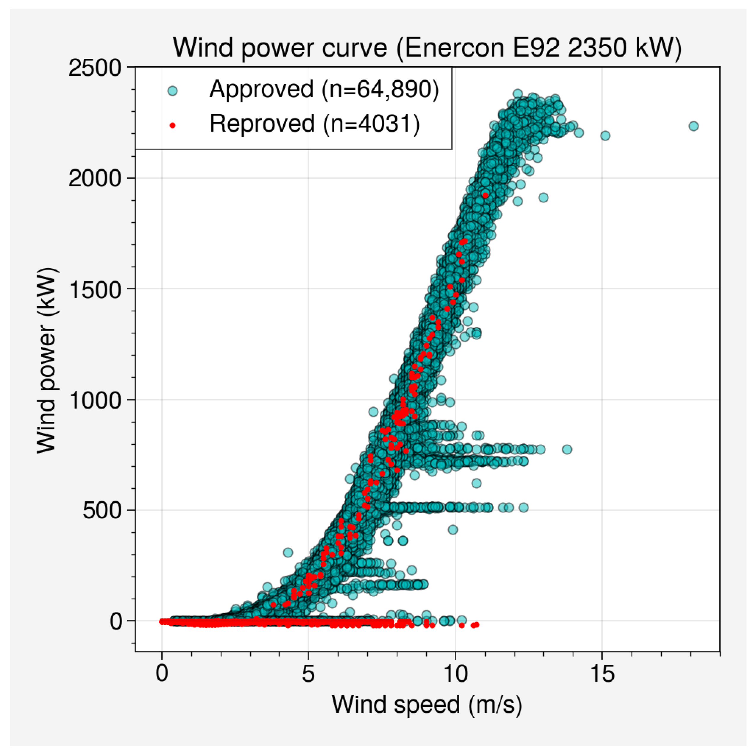
Figure 5 displays the average statistical metrics (RMSE, NRMSE, MB, R
2) obtained by comparing the predicted wind power to the observed values across all 24 time steps. The results indicate that the optimal methodology in this scenario is the error correction, evidenced by its lowest error values (e.g., the RMSE and NRMSE), indicating that its predictions align more closely with actual wind power values in short-term forecasts. In addition, its highest R
2 values suggest that a larger proportion of the total variance in the wind power data is explained by its forecasts, which reinforces the notion that the error correction approach provides a more precise forecast in the short-term.
Both approaches exhibit a reduced bias (values closer to zero) across all predictions, when comparing to the base model, suggesting fewer systematic errors and superior calibration when compared to the second approach. While the base model underestimates the values, the proposed approaches overestimate them, but in lower magnitude.
Table 2 displays the statistical metric values derived from both the combined approaches and the base model (KNN). Although the models predicted 24 time steps (which corresponds to 12 h ahead with 30 min frequency), only the 2nd, 6th, 12th, and 24th time steps are presented for clarity, as shown in
Figure 4.
The error correction model (second approach) consistently had the lowest RMSE values across time steps, when compared to the error prediction model (first approach), and the KNN base model. Specifically, the RMSE values for the error correction model ranged from 281.06 to 425.40 kW, while the corresponding range for the KNN model was 312.27 kW to 481.31 kW and for the error prediction model was 295.87 kW to 448.07 kW. The error correction model also demonstrated superior performance in terms of the NRMSE. It registered values between 44.48% and 69.53% across time steps. Conversely, the base model presented NRMSE values ranging from 46.94% to 74.69% and the error prediction model had values between 44.48% and 66.01%.
Our study’s findings are consistent with the existing literature in the domain of wind power prediction. Specifically, Ref. [
18] employed a KNN wind power prediction model leveraging multi-tupled meteorological input data and achieved an NRMSE of 17.8% for a 10-min ahead forecast. As aforementioned, our KNN base model’s NRMSE values were lower for 30 min ahead. Considering this time horizon, the EC approach yielded 31.15%, while the second (EP method) recorded 32.26%. For the 12-h-ahead prediction, these figures were 59.12% and 61.38% for the first and second approaches, respectively.
In the literature, a clear consensus on the normalization of metrics has yet to be reached. In our work, we opted to calculate the RMSE normalization based on the magnitude of the data, specifically by dividing it by the capacity range (difference between the maximum and minimum) observed in the dataset. This approach aligns with the method used in [
18]. However, it is worth noting that certain other papers utilize a different normalization by the installed capacity, which is more tailored to the operational environment’s reality [
19,
21].
Notably, Ref. [
21] had achieved NRMSE values ranging from 9.01% to 20.53% depending on the model, methodology, and prediction horizon used for multistep forecasting. On the other hand, in [
19] were developed multiple time step predictions up to 48 h, refining NWP predictions, and an NRMSE of less than 20% was consistently achieved.
Finally, the absolute value was considered for the bias evaluation to inform the degree of variation of the forecasts from the actual measurements, regardless of the direction of deviation. In this sense, the error correction model exhibited relatively lower absolute values of the bias in comparison to the base model, with values ranging between 42.81 and 78.00 kW, whereas the bias of the base model had a greater variation from 42.25 to 109.07. Nevertheless, the best performance of bias was achieved by the error prediction model with absolute bias values between 28.04 and 66.34.
Table 3 compares the performance improvements of both models (the error prediction model and the error correction model) to the base model for the error metrics RMSE and bias. It was unnecessary to include the NRMSE, as its improvement is the same as RMSE.
Relative to the base model, both models demonstrated enhancements with respect to the error metrics across the time steps. The error prediction model (first approach) presented improvements in the RMSE ranging from 5.25% to 9.47%. On the other hand, the error correction model featured a greater enhancement, spanning from 9.99% to 13.19%. An examination of the bias improvement degree reveals that the error prediction model showed significant enhancements, with values extending from 33.63% to 78.01% across the evaluated time steps. The error correction model started to show improvements in the 3 h ahead forecast: the values ranged between −1.34% and 56.69%. On average, the error prediction model demonstrated an overall degree of improvement of approximately 8.06% in the RMSE, and 51.12% in bias. Concurrently, the error correction model, on average, achieved notable progress with 11.43% in the RMSE and 48.19% in bias.
In conclusion, both the error prediction and error correction models displayed remarkable advancements across all evaluated metrics and time steps. The error correction model registered more pronounced progress in the RMSE index, while the error prediction model demonstrated significantly higher enhancements in the bias value.
This might be because the error correction model consistently overpredicts, generating a positive bias of high magnitude. These consistent overpredictions indicate that while the model’s predictions are always above the actual values, the RMSE and NRMSE remain relatively low, for they are not erratically far from the truth.
On the other hand, the error prediction model bias is closer to zero, combined with its high error metric values, which indicates that its predictions do not consistently lean in one direction. Instead, the model’s predictions oscillate between underpredicting and overpredicting, which averages out to a bias nearer to zero.
4. Summary, Conclusions and Future Work
The present study focused on the short-term wind power forecasting, evaluating two machine learning correction approaches, namely the error prediction (first) and the error correction (second) methods, aiming to highlight their capability for enhanced forecasting performance using a machine learning model, specifically a KNN model. A SCADA system dataset utilized in this work was collected by an Enercon E92 turbine at Casa Nova II wind farm in a semi-arid region, located near Sobradinho reservoir in Bahia state, Brazil.
Based on the analysis, when considering both metric values and the degree of improvement in error metrics, both the error prediction and error correction models demonstrated substantial progress compared to the base model across the examined time steps and metrics. The second approach exhibited superior metric results with lower errors and higher R2 values. The error prediction approach improved bias and the RMSE more than 78.01% and 9.47%, respectively, in comparison to the baseline machine learning model, KNN. Overall, this study contributes to the understanding of wind power forecasting methodologies and highlights the strengths and limitations of each approach. The findings emphasize the importance of considering requirements of the aimed problem to select the most appropriate methodology.
Some future research is worth exploring in the context of wind power forecasting based on data-driven machine learning approaches. Deep learning models, for instance, may offer improvements in accuracy due to their proficiency in representing temporal dependencies and nonlinear relationships which are latent within the data. Furthermore, the extension of forecasting analysis to encompass all turbines within a wind farm presents an intriguing avenue for improvement, mainly if other data are also available (i.e., weather stations). Integrating data-driven machine learning methods with deterministic forecasts, such as NWP models, could enhance predictive capabilities from intra-day to day-ahead time.

 ,
, 


