Article

Numerical Modeling and Application of Horizontal-Axis Wind Turbine Arrays in Large Wind Farms

1
College of Shipbuilding Engineering, Harbin Engineering University, 145 Nantong Street, Harbin 150001, China
2
Guangdong Haizhuang Offshore Wind Power Research Center Co., Ltd., Guangdong 524000, China
*
Author to whom correspondence should be addressed.
Wind 2023, 3(4), 459-484; https://doi.org/10.3390/wind3040026
Submission received: 3 August 2023 / Revised: 14 September 2023 / Accepted: 7 October 2023 / Published: 10 October 2023

Abstract

:
The global supply of energy is still tight, even with the rise of renewable energy utilization and abundant wind energy. More and more large wind farms have been installed globally. As of 2020, China’s total installed capacity accounted for 38.8%, far ahead of other countries. The layout of horizontal-axis wind turbine (HAWT) arrays in large wind farms poses three main issues: (1) How to select a site. (2) How to arrange the HAWT arrays to achieve greater power extraction at a specific wind farm. (3) How to reduce the noise generated by HAWTs. The numerical simulation of a HAWT wake field generally includes the analytical method (AM), vortex-lattice or vortex particle method (VM), panel method (PM), blade element momentum method (BEM), generalized actuator method (GAM), and direct modeling method (DM). Considering the computational cost, this paper combines DMs and mainly adopts the BEM-CFD coupling method, including uniform and non-uniform loading of axial force. Forty specially designed numerical experiments were carried out, which show that: (1) the BEM-CFD method greatly improves the calculation speed within the accuracy range of a thrust coefficient less than 2.5%, making it very suitable for the calculation of large wind farm HAWT arrays; (2) for regular HAWT arrays, it is reasonable to choose a 6 D spacing in the wind direction and a 4 D spacing in the crosswind direction for simplicity in practice.

1. Introduction

Wind field is a technical term used in environmental impact assessment to evaluate the inconsistency of local wind speed, direction, and other factors within a region. According to the causes of wind formation, there are various types of wind including sea–land wind, water–land wind, valley wind, and the urban heat-island effect [1]. When valley winds occur, they are often accompanied by a temperature inversion layer [2], and the atmosphere appears solid state, making it difficult for pollutants to dilute and diffuse. If pollutants are drawn into the circulating current, they will remain in the valley for a long time, causing serious air pollution events. In ancient China, there was a sacrificial wind field for the Naxi ethnic group in Yunnan. In the eyes of the Naxi people, the wind was a symbol of the divine power of nature, accompanying them like a shadow and always present. The power of the wind seemed endless. People placed their reverence for nature and their desire to protect it in wind-worship activities, and also used the power of the wind to transcend death, allowing a smooth ascent to heaven and return to their ancestors. In the past few decades, due to global energy shortages, the use of renewable energy has emerged. Wind energy is a type of renewable energy. More and more large wind farms using wind turbines have been installed globally. The total installed capacity of wind turbines in various countries around the world by 2020 is shown in Figure 1, including the sum of onshore and offshore capacity [3].
The layout of wind-turbine arrays in large wind farms poses three main issues: (1) How to select a location; it is necessary to simulate the Earth’s wind field in order to select a suitable location for arranging wind-turbine arrays. (2) How to arrange a wind-turbine array to achieve greater power extraction at a specific wind farm. (3) How to reduce the noise generated by HAWTs. When simulating the wake field of a wind turbine, there is a significant difference between the far and near fields. The near wake is an area approximately 1 ~ 2 D ( D is the rotor’s diameter) downstream from a wind turbine, where the geometry of the wind turbine directly affects the flow field, resulting in a different blade tip-vortex; the tip-vortex and root-vortex lead to large velocity gradients and extreme turbulence intensity; for a very high tip speed ratio (TSR), the tip-vortex produces a continuous vorticity-sheet and a shear-layer. In the far wake, the axial velocity decreases while the turbulence intensity increases, which can only indirectly feel the impact of the actual wind turbine shape. Turbulence is the main physical process in the far wake of a wind turbine, which generally comes from three sources: (1) atmospheric turbulence, coming from the roughness of the Earth’s surface and thermal effects; (2) mechanical turbulence, coming directly from the wind-turbine blades, nacelle, and tower; (3) wake turbulence, resulting from the breaking down of the wind-turbine blade tip-vortex. Turbulence, as an effective mixer, can restore velocity-loss and reduce turbulence intensity overall. In the far downstream, the velocity deficit becomes approximately axisymmetric, Gaussian and shows self-similarity. Wake meandering [4] is a large-scale motion, which is believed to be driven by large-scale turbulent structures, and it may further reduce loss of velocity, although it greatly increases the fatigue and ultimate load of downstream wind turbines.
High power wind turbines are usually HAWTs. HAWTs can be divided into micro, mini, household, commercial small-scale, commercial mesoscale, commercial large-scale, and commercial super-large-scale types according to the diameter of the rotor [5]. The HAWT used in this study belongs to the commercial mesoscale type. Some researchers have studied the influence of large-scale wind farms on climate conditions and concluded that the installation of large-scale wind farms using wind turbines may have changed global climate conditions to some extent and had adverse effects on the atmosphere, changing surface temperature and rainfall to some extent [6,7,8]. It is reasonable to assume that the flow field of a wind turbine is incompressible, as the wind-speed upstream and downstream of a wind-turbine placed in the atmosphere is usually within the range of 5–25 m/s. This compressibility effect may be important only when calculating the aerodynamics of the blade tip. For non-neutral atmospheres, Boussinesq approximation is commonly used to explain buoyancy effects, and additional equations of temperature must be solved. The Earth’s rotational effect expressed using the Coriolis terms is often ignored in many wind-turbine-wake studies, but this can have a certain impact when studying large wind farms using wind turbines.
In the atmospheric boundary layer (ABL), the maximum turbulence scale is 1 km, while the minimum turbulence scale is 1 mm. However, in the blade boundary layer, the minimum scale is even smaller. The scale-range of turbulence depends on the Reynolds number (Re). The large Reynolds number encountered in wind-turbine-wake calculations results in a large-scale range, which makes computer simulation very expensive. Therefore, it is not feasible to use the so-called direct-numerical-simulation (DNS) [9] to solve all scales in the flow. It is necessary to build a turbulence model and model the unsolved small-scale effects based on large-scale behavior. However, even if a turbulence model is used to reduce calculation costs, the boundary layer on the wind-turbine blade and the turbulence structure in the wake flow cannot be solved at the same time. We need to simplify representation of the wind turbine in wake calculations and representation of the wake in boundary layer calculations of the blade. Research shows that mechanical turbulence, atmospheric turbulence and wind-turbine-wake characteristics are likely to be very insensitive to the blade Reynolds number [10].
The aerodynamic numerical simulation of the wind turbine wake generally observes the following six methods: (1) Analytical method (AM) [11]; the blades are represented by setting a thrust coefficient, and the expressions of velocity deficit and turbulence intensity are obtained by using the self-similarity property of the far wake. (2) Vortex-lattice [12] or particle method (VM), assuming inviscid and incompressible flow, and describing the blades with vorticity concentrated in thin sheets or particles, with blade elements represented by lift lines or surfaces. (3) Panel method (PM) [13], also describing inviscid flow-field, but more accurately considering the geometry of the blade; the blade is represented by surface grids, and viscous effect can be included using a boundary-layer code. (4) Blade element momentum method (BEM) [14], which is an application of the quasi one-dimensional momentum theory for blade elements. (5) Generalized actuator method (GAM); in this method, a wind turbine rotor-blade is represented by a physical force superposed on the flow field, including the actuator disk (AD) [15], actuator surface (AS) [16], and actuator line (AL) model [17,18], as shown in Figure 2 below; this method avoids explicit calculation of the blade boundary layer, reduces calculation costs, and simplifies grid generation. (6) The direct modeling (DM) method, which discretizes actual blades on a computational grid for calculation, is the most reasonable method for calculating flow around the wind turbine through a body-fitted grid; direct modeling is also helpful in understanding the mechanism of fan-wake aerodynamics.
In the DM method, the blade is accurately represented. However, for an accurate simulation of the blade boundary layer, including transition, separation and stall, the calculation cost is very high. Moreover, the compressible effect at the tip needs to solve the compressible N-S equation, while the wake basically retains compressibility. The generation of a high-quality moving-body fitted-mesh is also a tough task. Mesh generation is generally carried out through what is known as overlapping or embedding grids, which communicate information with each other through different overlapping grids. This method is currently not applicable for calculation of the wind-turbine wake in large wind farm wind-turbine arrays. For the general actuator method, from the thrust coefficient required by the uniform-load AD to the local lift and drag coefficients required by the non-uniform-load AD and AL methods, and to the distribution of pressure and friction force required by the AS method along the chord length of blade section, improvements in accuracy are accompanied by a higher calculation cost and more detailed airfoil data. The steady-state characteristics of the AD method limit its application in Reynolds average Navier–Stokes equation simulation (RANS). The unsteady characteristics of the AL and AS methods make them very suitable for large eddy simulation (LES). Considering the computational cost, the AL and AS methods are applied to the study of a single wake field, and most wind turbine arrays in wind farms are simulated using the AD method. This article uses the BEM-CFD method, which is similar to the AD method.
From the above review, it can be seen that there have been many studies on modeling individual wind turbines and their flow fields, but few on the arrangement of wind-turbine arrays in large wind farms. Due to limited article length, our study aims to address two main issues:
  • Conducting theoretical research on various numerical simulation wind-turbine models, seeking feasible (with acceptable computational costs) wind-turbine models for large-scale wind-farm calculations, and selecting the BEM-CFD coupling method on the basis of balancing practicality, accuracy, and cost;
  • Customizing the solver in open-source OpenFOAM, applying the BEM-CFD coupling method to wind-farm calculations, studying the impact of different array wind-turbine arrays on wind farms and the interaction between wind-turbine arrays, and drawing some very practical conclusions.
The research objective is to provide certain strategies for selecting and arranging HAWTs in practical scenarios, as well as optimizing the design of wind turbines in wind farms, both of which have strong practical significance.

2. Research Method

This section introduces the experimental HAWT geometrical characteristics, control equations of flow field around HAWT, HAWT modeling, and numerical experimental settings adopted by the research.

2.1. Description of Experimental HAWT

Our study has adopted a commercial mesoscale Nordbank NTK 500/41 three blade (B = 3) wind turbine [19], which is a fixed pitch and stall adjustment type with a rotor radius of R = 20.5 m and a hub center height of h h u b = 35.0 m, with cut-in wind-speed of 4 m/s and cut-out wind-speed of 25 m/s, and a rotating speed of n = 27.1 rpm; the relative chord length ( c = c / c t i p ) and torsion angle ( β ) distribution of airfoil-sections along the blade span are shown in Figure 3a. Two six-digit laminar flow airfoils, NACA63-210 and NACA63-412, are used, and their lift and drag coefficients at different angles of attack and Reynolds numbers are calculated, as shown in Figure 3b–d. The lift coefficient of the NACA63-210 airfoil becomes more stable with the increase in the Reynolds number, and the stall angle also increases, while the un-steady region tends to be stable at a certain Reynolds number. At Re = 10 6 , lift, the coefficient of the NACA63-412 airfoil is slightly larger than that of the NACA63-210 airfoil at different angles of attack, and they are basically parallel. The drag coefficient of the NACA63-210 airfoil decreases along with an increase in the Reynolds number. At Re = 10 6 , the difference between the drag coefficients of the two airfoils is very small, and the drag coefficient is one to two orders of magnitude smaller than the lift coefficient.

2.2. Governing Equation of Flow Field

The calculation of the wind-turbine wake-field is based on numerical simulation of the N-S equations system, and the turbulence model adopts the k ω SST model in the RANS equation system, which is different from the LES in that it uses statistical averaging in time rather than spatial averaging. For Newtonian fluids, based on the Boussinesq hypothesis, that is, the Reynolds stress is a linear function of the average velocity-gradient; the Reynolds stress tensor can be directly modeled. For incompressible fluids, it can be simplified by introducing turbulent kinetic energy k and turbulent eddy viscosity μ t which is analogous to molecular viscosity, and length scale l can be used to represent μ t . Based on this representation, models can be divided into an algebraic model, one-equation model, two-equations model, and second-order closed model. Each model has its own advantages and disadvantages, and no model is universally applicable to all flow conditions. The two-equations model is the most popular in industrial applications, which solves two transport equations to solve μ t .
The k - ε model is the earliest and most popular of the two equation models. In the derivation process, it is assumed that flow is completely turbulent, and the molecular viscosity effect can be ignored. Therefore, this model is a high Reynolds-number model, which is only applicable to completely turbulent free-shear flow, and cannot be integrated to the wall (low Reynolds-number). It is also necessary to add damping functions or additional source terms to the equation of turbulent dissipation ε . In the two-equations model, stagnation point anomalies may occur, and the generation of turbulent kinetic energy may be overestimated when the intermediate level k encounters a large strain rate, which may be due to an overestimation of μ t or undervaluation of sink terms. To overcome this problem, a local turbulence time scale t s =   k / ε is introduced. Replacing ε with ω (the rate at which turbulent kinetic energy is converted to internal thermal energy per unit volume and time) yields the k ω model, which can be better applied to the calculation of separated flows with inverse pressure gradients. This model is sensitive to any defined ω in free flow, while the k - ε model does not have this problem. There are many modified and improved versions of k - ε model and k ω model. Considering the advantages and disadvantages of these two models, we can combine these two models for modeling, and then we get the BSL k ω model. This model is similar to the k ω model for boundary layer flow, and almost equivalent to k - ε model for free shear flow. In order to improve the influence of the reverse pressure gradient, Bradshaw’s hypothesis [20] is adopted; that is, main shear stress and turbulent kinetic energy in boundary layer are linearly correlated through the relation τ x y = ρ a 1 k to yield the SST k ω model used in this article. In physical space, the velocity field in the Cartesian coordinate system x = ( x 1 , x 2 , x 3 ) is u = ( u 1 , u 2 , u 3 ), and the equations for mass conservation and momentum conservation are respectively
u i , i = 0 ;   i = 1 , 2 , 3
u i , t + ( u i u j ) , j = p , i + ( ν + ν t ) ( u i , j + u j , i ) , j + f i ;   i = 1 , 2 , 3
where p = P / ρ is static pressure; ν is the kinematic viscosity of air molecules, assuming that ν is constant and uniform; ν t is the turbulent kinematic viscosity; f i or f is the physical force used to represent effect of wind turbine blades on convective field. Note that the relationship between kinematic viscosity ν and dynamic viscosity μ is ν = μ / ρ , and ρ is the density of air at normal temperature and standard atmospheric pressure. Two transport equations of the SST k ω model are
( ρ k ) , t + · ( ρ u k ) = · ( μ e f f . k k ) + P k β * ρ k ω
( ρ ω ) , t + · ( ρ u ω ) = · ( μ e f f . ω ω ) + C ¯ α P k ( ω / k ) C ¯ β ρ ω 2 + 2 ( 1 F 1 ) σ ω 2 ( ρ / ω ) k
where μ e f f . k = μ + μ t / σ ¯ k , μ e f f . w = μ + μ t / σ ¯ ω , μ t = ρ k / ω , k t = μ t / P r t , blending function F 1 = tan h ( γ 1 4 ) , γ 1 = min [ max [ k / ( β * ω d ) , 500 ν / ( d 2 ω ) ] , 4 ρ σ ω 2 k / ( C D k ω d 2 ) ] , d is the vertical distance from the wall surface, C D k ω = m a x [ 2 ρ σ ω 2 ω 1 k · ω ,   10 10 ] . All coefficients depend on the mixing function F 1 , which can be defined as ϕ ¯ = F 1 ϕ 1 + ( 1 F 1 ) ϕ 2 . Note there are model coefficients in the original SST kω model: C α 1 = 5/9, C β 1 = 0.075, β * = 0.09, σ k 1 = σ ω 1 = 2, P r t = 0.9; Model coefficients in the RANS-BSLkOmega model: Cα2 = 0.4404, C β 2 = 0.0828, σ k 2 = 1.0, σ ω 2 = 0.856, P r t = 0.9; Model coefficients in the k - ε model include: C ε 1 = 1.44, C ε 2 = 1.92, C μ = 0.09, σ k = 1.0, σ ε = 1.3, P r t = 0.9.

2.3. HAWT Modeling

In order to better illustrate the coupling simulation method of BEM and CFD used in this article’s calculation, this section includes three parts: (1) An introduction to one-dimensional momentum theory, which omits the detailed derivation process of one-dimensional momentum theory (readers who need it can deduce it themselves or send an email to the author requesting the derivation process file), only providing some important conclusions. (2) The classic BEM method is briefly presented, and a more detailed derivation process can be found in [21]. (3) The BEM-CFD method is given, which should be distinguished from the classical BEM method.

2.3.1. One-Dimensional Momentum Theory

In a one-dimensional model, the rotor is modeled as an ideal permeable disk (PD), which is frictionless and has no rotational velocity component in the wake. The PD acts as a drag device to drive wind speeds from U 0 far-upstream of the rotor to u at the rotor plane, and u 1 in the far wake. Therefore, the streamline is divergent, as shown in Figure 4a. Resistance is obtained by pressure drops on the rotor, and there is a small pressure rising upstream of the rotor, from atmospheric level p 0 to p , then there is a discontinuous pressure dropping at the rotor, and pressure downstream of the rotor continuously increases to atmospheric level. Assume that Mach number (Ma) is small, so density of air is constant, and the axial speed must change from U 0 to u 1 continuously. Typical distribution of axial velocity and pressure is shown in Figure 4b. Due to this assumption of an ideal rotor, we can take control-volume C V 1 (thin solid line, taken along the streamline) or C V 2 (thin dashed line, square zone) as shown in Figure 4c, where A is area of the rotor disc. The axial induction factor a satisfies the equation u = ( 1 a )   U 0 . According to the Bernoulli equation (from upstream to rotor tight front, from rotor tight rear to downstream), the relationship between the velocity U 0 , u 1 , u , thrust T and absorbed shaft power P can be easily derived. The effective power in a cross-section is calculated using P e = 0.5 ρ A U 0 3 , where A is area of the rotor disc, through which dimensionless power coefficient C P and thrust coefficient C T can be defined. To calculate the extreme value of C P about a , and obtain that when a = 1/3, there is a maximum value of C P . m a x = C P . B e t z = 16/27, this maximum value is called the Betz limit. We obtain
u = 0.5 ( U 0 + u 1 ) ,   u 1 = ( 1 2 a ) U 0
T = 2 a ( 1 a ) ρ U 0 2 A ,   P = 2 a ( 1 a ) 2 ρ U 0 3 A
C P = P / P e = 4 a ( 1 a ) 2 ,   C T = T / ( 0.5 ρ A U 0 2 ) = 4 a ( 1 a )
Simple one-dimensional momentum theory is not applicable to cases where a > 0.3 ~ 0.4 . The reason is that when velocity jump ( U 0 u 1 ) is too high and then vortices are formed, free-thin shear-layer at edge of the wake becomes unstable, thereby transferring momentum from external flow to the wake. The state in this situation is called a turbulent wake state [22], and this article only discusses the windmill state.
For an ideal rotor, there is no rotational component in the wake flow, but actual wind-turbine wake-flow has rotational effects. Let absolute speed after the rotor be ( C r , C θ , C a ) , where C θ is the azimuth component, as shown in Figure 5a with u the axial velocity passing through rotor. Note we have U a = C a = u. Axial speed of the rotor is given by axial induction factor a . By assuming that the rotating speed of the wake can also be given by another induction factor a , i.e., C θ = 2 a ω r , then we can obtain d P = 2 π r 2 ρ u ω C θ d r = 4 π a ( 1 a ) ρ U 0 ω 2 r 3 d r , total power and power-coefficient can be expressed respectively as
P = 4 π ρ U 0 ω 2 0 R a ( 1 a ) r 3 d r , C P = ( 8 / λ 2 ) 0 λ a ( 1 a ) x 3 d x
where, λ (= ω R / U 0 ) is the tip speed ratio, x (= ω r / U 0 ) is the ratio of local rotating-speed to wind-speed. For given power P and wind speed U 0 , azimuth velocity-component C θ in wake decreases as rotating speed ω increases. So, from an efficiency perspective, it is necessary to have a high-rotating wind turbine to minimize loss of kinetic energy contained in the rotating wake. In order to optimize power, it is necessary to maximize the expression f ( a , a ) = a ( 1 a ) . If local angle of attack is less than the stall angle, a and a are not independent, and the relationship x 2 a ( 1 + a )   = a ( 1 a ) which can be directly derived from Figure 5b is used, the optimal relationship between a and a can be simply derived as a = ( 1 3 a ) / ( 4 a 1 ) . Relationship between a , a and x is shown in Figure 5c. It can be seen that as rotating speed ω increases, x (= ω r / U 0 ) also increases, the optimal value of a tends to 1/3; this value is consistent with that of simple momentum theory of an ideal rotor. Calculate the relative optimal power coefficient C P / C P . m a x through integral Equation (8). The results are shown in Figure 5d. It shows that when λ > 6, the loss caused by rotating is relatively small. Note: θ represents the local pitch angle of the blade, that is, the local angle between chord and rotor rotation plane, which can be expressed as θ = θ P + θ T , with θ P the angle between blade-tip chord and the rotor plane, θ T the torsional angle measured relative to chord of the blade-tip. ϕ is the angle between rotation plane and relative velocity U r e l , then a local attack angle α(= ϕ θ ) can be determined. It is worth noting that in 1935, Glauert [23] also conducted research on wind-turbine power under different λ , his results are basically consistent with the results in Figure 5d. Burton and colleagues [24] believe that for all tip speed ratios, when a = 1/3, the maximum value of C P is 16/27, independent of the tip speed ratio.

2.3.2. Classic BEM Method

Classical BEM theory uses global momentum balance and two-dimensional blade elements to calculate the aerodynamic characteristics of blades. It can calculate stable loads under different wind speeds, rotating speeds and pitch angles, and then calculate thrust and power. In order to calculate the time-series of time-varying input loads, engineering models must be added. In one-dimensional momentum theory, the actual geometric shape of the rotor, such as the number of blades, the distribution of twist and chord, and the airfoil used, is not considered. The BEM method combines momentum theory with local events that occur in actual blades, discretizing flow tubes into annular height elements ( d r ). Lateral boundaries of these elements are streamlined, implying there is no flow between the elements. We make these assumptions: (1) There is no radial dependency, meaning that what happens in one element cannot be felt by other elements; (2) For each annular element, the force exerted by the blades on the flow is constant, corresponding to a rotor with countless blades, while actual rotor blades are finite.
The derivation of all necessary equations for both steady and unsteady BEM models can be found in [21], and only the calculation steps for steady BEM are briefly provided here. For unsteady BEM, time iteration is introduced by considering the dynamic stall model, dynamic wake model, and yaw model, without solving the flow field. Under the assumption that different control-volumes are independent, each annular band can be computed separately. Before solving for another radius, the solution at one radius can be calculated. For each control volume, the steady BEM is calculated using the following eight steps:
  • Initialize a and a , usually a =   a = 0;
  • Calculate flow angle ϕ according to Figure 5b;
  • Calculate the local angle of attack α according to Figure 5b;
  • Find and read C l ( α ) and C d ( α ) from the given table;
  • Calculation C n = p N / ( 0.5 ρ V r e l 2 c ) = C l cos ϕ + C d s i n ϕ and C t = p T / ( 0.5 ρ V r e l 2 c ) =   C l sin ϕ C d c o s ϕ ;
  • Calculate a = 1 / ( 4 s i n 2 ϕ / ( σ C n ) + 1 ) and a = 1 / ( 4 s i n ϕ cos ϕ / ( σ C t ) 1 ) , where, solidity σ is defined as proportion of annular area covered by blades in the control volume, i.e., σ ( r ) = c ( r ) B / ( 2 π r ) , wherein B the number of blades, c ( r ) the local chord length, and r the radial position of the control volume;
  • If a and a have changed by more than a certain margin of error, proceed to step 2 or complete;
  • Calculate the local load of blade segments.
Above is the basic algorithm of BEM method. In order to get a better result, the algorithm needs to be modified twice (affect step 6 of the BEM algorithm):
  • Ludwig Prandtl’s tip loss factor. It corrects the assumption that the number of blades is infinite. The derivation of it is very complicated, but a complete description can be found in [21]. Therefore, when the corrected load is uniformly distributed along the azimuth and used for the momentum equation, their blade induction results are very similar to the case of a finite number of blades by using a = 1 / ( 4 F s i n 2 ϕ / ( σ C n ) + 1 ) and a = 1 / ( 4 F s i n ϕ cos ϕ / ( σ C t ) 1 ) , where F is correction factor for aerodynamic loads;
  • Glauert correction. It is an empirical relationship between thrust coefficient C T and axial induction factor a , when a > 0.2~0.4, simple momentum theory fails, and the relationship derived by one-dimensional momentum theory no longer holds.

2.3.3. BEM-CFD Coupling Method

Whether uniform or non-uniform axial-loads, the BEM-CFD coupling method can introduce tangential forces on the surface of the ideal rotor to account for rotational effects. The study by [25] showed that for uniformly distributed loads, including rotational and non-uniform loads in the prediction of average velocity and turbulence intensity can lead to significant improvements, especially in the near-wake center. A uniformly loaded rotor leads to an underestimate of wake-loss and turbulence intensity, and effects of rotational and non-uniform loads basically disappear downstream. The research of [26] applied it to LES simulation and showed that the influence of tangential force on wake flow appears to be negligible in cases of medium power-coefficient and high tip-speed-ratio. Considering that, in large wind-turbine wind farms, more attention is paid to the power output of the actual wind-turbine array and downstream wind-turbine characteristics in the slightly distant wind-turbine wake-flow-field, the model used in this article does not include tangential forces and only loads axial uniform or non-uniform loads. The boundary layer is not explicitly simulated, but its influence is considered through lift and drag coefficients, which greatly reduces the computer resources required.
This method is different from the classical BEM method, where, U r e f is obtained through an iterative process using global momentum balance, and Prandtl blade loss correction and Glauert correction for high axial induced velocity are applied. In the calculation of N-S equations, this is unnecessary because the flow field will take the presence of blades into account, and therefore induction will automatically change. A flow chart of the BEM-CFD method is shown in Figure 6a. However, using two-dimensional airfoil data still requires calibration in order to obtain the correct flow angle and velocity [22]. A related issue is to determine local α to find c L and c D , and [27] developed a technique that can determine α based on information slightly upstream of the rotor.
The implementation of the BEM-CFD method is achieved using a custom solver (windFarmLienFoam) on the open-source software OpenFOAM, using a finite volume calculation method. In the custom solver, the force applied to the blade is loaded into uniform or non-uniform volume cells in the rotor plane, that is, f i is added to Equation (2). When subjected to non-uniform loading, as shown in Figure 6b, thrust distribution is assumed to be T ( r ) = ( C 0 + C 1 r 2 + C 2 r 4 ) T , where, r is the local radius of the rotor, T is the thrust calculated through uniform loading, and C 0 = 0.1, C 1 = 0.5 and C 2 = 0.01 is a polynomial coefficient.

2.3.4. Jensen Wake Model

To demonstrate the reliability of the BEM-CFD coupling model, here is a brief introduction to the Jensen wake model [28] for subsequent comparison. The Jensen wake model is briefly described in Figure 6c. The wake effect between two turbines, with the upstream i wind turbine ( W T i ) and downstream j wind turbine ( W T j ) located at coordinates ( x i , y i ) and ( x j , y j ) , respectively. Assuming that the wake effect is axisymmetric, its strength depends on the distance and wind direction between the two turbines. Wind speed at downstream W T j position x j is determined using the following formula:
u j = u i ( z ) ( 1 i N j ( 2 a / ( 1 + k x i j / r j ) 2 ) 2 )
where, u i ( z ) is incoming wind-speed at the shaft height z of upstream W T i , N j is numbers of all upstream HAWTs that affect W T j . The Jensen model assumes a linear expansion of the downstream wake zone, so the wake radius at the downstream W T j position is r j =   k x i j + r i with r i the radius of upstream W T i , x i j the distance measured along wind direction between HAWTs i and j . k is a dimensionless parameter that determines the expansion rate of the wake region, the value of which is calculated from the empirical formula k = 0.5 / ( ln ( z / z 0 ) ) proposed by Frandsen et al., where z 0 is the length of surface roughness, which depends on the terrain characteristics. If the terrain information of the pre-installed location of the wind turbine cannot be accurately obtained, generally, k = 0.075 is taken for onshore wind turbines, k = 0.05 is taken for offshore wind turbines, and the value of water roughness is usually 0.0002, although it may increase with changes in sea conditions. a is axial flow induction factor of the HAWT, which relates to the thrust coefficient C T , there is a = ( 0.51 1 C T ( u i ) ) , where C T ( u i ) is the thrust coefficient of the i -HAWT that varies with wind speed. The Jensen model assumes that the wake region of the HAWT is in a fully turbulent state and ignores the blade-tip vortices generated by the HAWT, so its applicable range is the far-wake region, which is the area after 3 D downstream of the HAWT, where D is the HAWT diameter.

2.4. Numerical Experiments Setting

2.4.1. Calculating Domain

A total of 40 numerical experiments were carried out in this paper, including a single HAWT, two HAWTs at the front and back, two HAWTs at the left and right, three staggered HAWTs, a three-rows and three-columns HAWTs array, and a one-row and three-columns HAWTs array in random mountainous areas with ABL, as shown in Table 1. The setting of the calculation domain is shown in Figure 7, where D is diameter of the HAWT rotor, d 1 is the distance between front and rear HAWTs, d 2 represents the distance between left and right HAWTs, ( x , y , z ) represents Cartesian coordinate system, and flow direction points towards the positive x -axis.

2.4.2. Meshing

For the DM method of a single HAWT, use three-level grid zones as shown in Figure 8a, with total grid numbers of approximately 7.6 million. Coarse to fine grid zones are region 1, region 2, and region 3, respectively. Grid sizes of these three zones are approximately δ x δ y δ z 0.1 D , δ x δ y δ z 0.0125 D and δ x δ y δ z 0.00625 D , respectively. The meshing of BEM-CFD method is shown in Figure 8b. The coarse grid size of a single HAWT is approximately δ x 0.36 D and δ y δ z 0.41 D , and the internal refine grid size is approximately δ x 0.045 D and δ y δ z 0.052 D , gradually transitioning from coarse to fine grids. For other multiple HAWTs, the grid size setting is similar. After the grid is divided, the grid cells are renumbered before calculation to reduce bandwidth and accelerate the calculation process.

2.4.3. Initial and Boundary Conditions

To accelerate convergence, the initial velocity of the flow field is set to (10 0 0) m/s. The boundary conditions for the DM method of single HAWT calculation with cases (1–3) are: (1) at the inlet, with a fixed uniform flow velocity U x = (10 0 0) m/s and zero pressure gradient; (2) at the outlet, it is the pressure inlet and outlet velocity, and fixed value pressure; (3) the boundary layer on the wall surface of the HAWT blades or nacelle is not directly calculated, and the wall function and zero pressure gradient are used; (4) elsewhere, a slip boundary is adopted, as shown in Table 2. The BEM-CFD method with case (4–40) does not have blade or nacelle walls, and other initial and boundary conditions are the same as the DM method, except for the bottom surface of case (40), as described in Section 3.3.2.

2.4.4. Schemes and Algorithms

For transient calculations, the algorithm of pressure-implicit-with-splitting-operators method (PISO) is used to solve N-S system Equations (1) and (2) and two transport Equations (3) and (4) of the turbulence model. A second-order implicit Crank–Nicholson method is used for time discretization. Space adopts a standard finite-volume discretization of Gaussian integral, and the value from cell-center to face-center takes linear interpolation. The gradient is limited, so that when the calculated gradient is used to extrapolate cell-value to face-value, face-value will not exceed the range of values in the surrounding cells, thus ensuring boundedness. In order to maintain second-order accuracy, explicit non-orthogonal correction is taken for non-orthogonality grids. The pressure Poisson-equation is solved by using a geometric aggregated algebraic multi grid (GAAM) method. For steady-state calculations, the semi-implicit method for pressure-linked equations method (SIMPLE) is used to solve the N-S system Equations (1) and (2) and the two transport Equations (3) and (4) of the turbulence model; there is no time discretization term, and other discretization is similar to transient calculations.

3. Results and Discussion
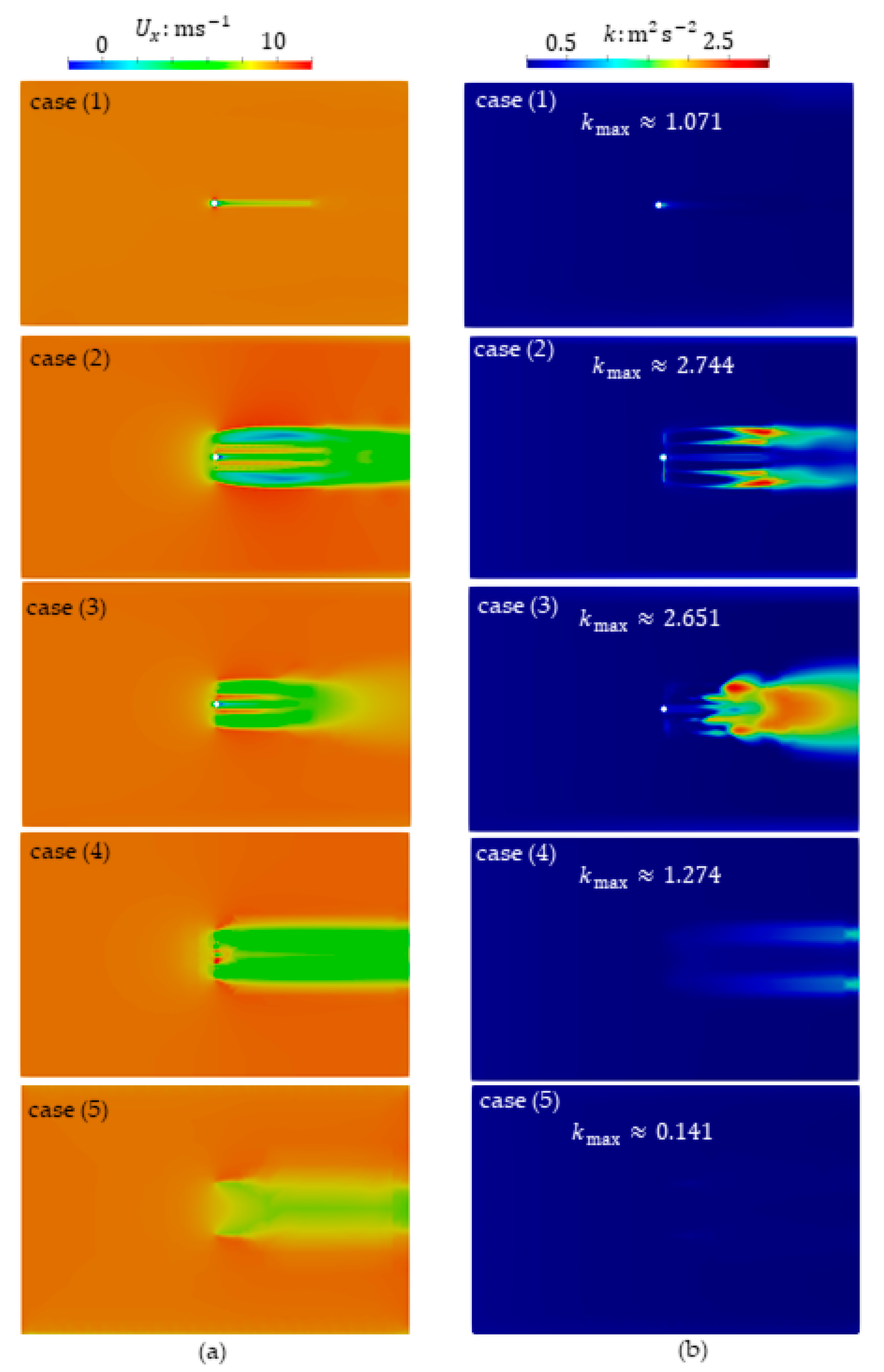
3.1. Single HAWT

In order to demonstrate the reliability of the BEM-CFD method in large-scale wind farms, five single HAWT cases were specially designed. Case (1) is only a sphere nacelle of radius 0.12 R ; case (2) and case (3) are a sphere nacelle with three blades of NACA63-412 or NACA63-210 for the blade airfoil; all of these three cases use the DM method. Case (4) and case (5) adopt the BEM-CFD method with uniform or non-uniform loading. The inlet of cases (1–5) is a uniform fixed speed U x = 10 m/s; the HAWT rotating speed and blade tip speed ratio are n = 0.452 rps and T S R = 5.818, respectively. The HAWT advance speed coefficient is J = U x / ( n D ) = 0.54. Case (6–14) adopts the BEM-CFD method with uniform loading, and there is still U x = 10 m/s, but the HAWT rotating speed is different in range of T S R = 4~12 integers. Note that the blade airfoil of cases (4–40) adopts NACA63-412.

3.1.1. Thrust Coefficient and Calculation Cost

Comparison of thrust coefficients and calculation costs between the single wind-turbine DM method with cases (1–3) and the uniformly or non-uniformly loaded BEM-CFD method with case (4) or case (5) is shown as Table 3. Based on results listed in the table, the following five main conclusions can be drawn:
  • Under the same HAWT geometry, the thrust coefficients calculated by the uniformly loaded BEM-CFD method with case (4) are larger than those calculated by the DM method with case (2), due to the underestimation of wake defects and turbulence intensity when using the BEM-CFD method;
  • The DM method with case (2) needs more time-cost in order to converge to a sufficient accuracy value (based on the clock time taken by the computer to calculate until t = 0.66 s as the standard). Cost of DM method is about 5042 or 90 times that of the uniformly-with-case (4) or non-uniformly-with-case (5) loaded BEM-CFD method;
  • Using the results of the DM method with case (2) as a reference value, the relative errors of the thrust coefficients of the uniformly loaded BEM-CFD method with case (4) and the non-uniformly loaded BEM-CFD method with case (5) are 1.8% and 2.1%, respectively. (Here, non-uniform loading has a certain degree of arbitrariness, so the error is slightly larger. It is possible to achieve better or worse results by assuming different thrust-distribution functions);
  • In the DM method, the thrust coefficient of case (2) with NACA63-412 is greater than that of case (3) with NACA63-210 when the rotor blades of the HAWT adopt different airfoil sections and other settings are the same, which is because the lift coefficient of airfoil NACA63-412 is greater than that of airfoil NACA63-210;
  • The thrust coefficient of a single nacelle in case (1) is approximately 0.6% of the nacelle and blades combination in case (2), and its impact can be almost ignored.
From the above five results, it can be concluded that after balancing the cost calculation, the BEM-CFD method is very practical in engineering, regardless of whether the force is uniform or non-uniform.

3.1.2. Calculated and Measured Power

Calculation and measurement values of HAWT power are shown in Figure 9a. It can be seen that shaft power of a HAWT with T S R 6 calculated through the BEM-CFD method is basically consistent with the classical BEM method and measurement results. Figure 9b shows the variation of measured and computed power coefficient with the tip-speed-ratio λ , while Figure 9c shows the variation of measured power coefficient with reciprocal of the tip-speed-ratio. It can be seen that the results start to diverge after case (11) due to using the same grid for cases (6–14) for convenience. The results of cases (11–14) are no longer valid. In order to converge the results, either a new refined grid is needed, different rotor modeling methods must be used for calculation, or certain modifications can be made directly. Regardless of the method used, the calculation results can be consistent with the measured values again. There is no need to do more cases here, because in the later calculation of HAWTs arrays in large wind farms, there is always a hypothesis of a < 0.221.

3.1.3. Axial-Velocity and Turbulent-Kinetic-Energy Field

Axial-velocity U x and turbulent kinetic energy k of cases (1–5) are shown as Figure 10. Case (1–3) take, respectively, t = 0.645 s, t = 0.66 s and t = 0.327 s. Case (4) and case (5) are steady calculations. As shown in the figure, compared with a separate nacelle for case (1), the axial velocity at the hub of the HAWT with nacelle and blades for cases (2,3) decreases more. When there is only the nacelle of sphere shape for case (1), there is a small turbulent kinetic energy region immediately behind the nacelle. However, in the presence of blades in cases (2,3), this small turbulent kinetic energy region weakens. When different blade cross-section airfoils are used and other conditions are set the same, the wake-velocity loss of case (2) with NACA63-412 at t = 0.66 s is more than that of case (3) with NACA63-210 at t = 0.327 s. This is due to the different blade airfoil cross-section characteristics of the two, and on the other hand, due to the insufficient calculation time of case (3), which was specially designed by us to explain another physical phenomenon in the future. Compared with the DM method in case (2), the uniformly loaded BEM-CFD method in case (4) significantly averages the wake, especially in the near-field of the HAWT, while in the far-field it is reasonable to expect that the two will ultimately be similar. Compared with the BEM-CFD method with uniform loading in case (4), the non-uniform loading in case (5) reduces the velocity loss at the wake of the HAWT. Compared with case (2), there is a larger range of turbulent-kinetic-energy zones in the HAWT wake in case (3); this is because the calculation time taken by case (3) is smaller than that of case (2), which is intentional by us. However, in the near-wake region of the HAWT, the turbulent kinetic energy of the two is basically the same. This indicates from one side that the rotating wake turbulence of the HAWT can stabilize the flow. It can be predicted that as the calculation time of case (3) increases, the distribution of turbulent kinetic energy at wake of the two will tend to be similar to case (4)’s mode; note that the rotating flow field of the HAWT is a quasi-steady flow field. Maximum turbulent kinetic energy in the wake of the BEM-CFD non-uniformly loaded HAWT for case (5) is very small, about 0.141   m 2 s 2 , depending on the selection of thrust distribution form.

3.1.4. Flow Fields at Different TSRs

Comparisons of velocity components ( U x , U y , U z ) , pressure p , turbulent kinetic energy k , turbulent dissipation ε or ω , and turbulent viscosity ν t for different TSRs with case (6) and case (9) are shown as Figure 11. It can be observed that, when the incoming wind speed is fixed, as the HAWT rotating speed increases, axial velocity loss in the wake increases, corresponding to an increase in power of a single HAWT; from an efficiency perspective, it is necessary to have a fast-rotating-speed HAWT to minimize the loss of kinetic energy included in a rotating wake. The higher the rotational speed, the greater the pressure difference, and the greater the thrust coefficient and power coefficient of HAWT. Compared with case (9) at a higher rotation speed, the turbulent kinetic energy and turbulent viscosity of case (6) at a lower rotation speed are basically negligible. However, after scaling down and enlarging the case (6) scale, it can be seen that it follows roughly the same mode as case (9), which is also a manifestation of self-similarity to some extent. Note that ω = ε / ( C μ k ) , its mode is similar at different rotating speeds.

3.2. Two and Three HAWTs

3.2.1. Two HAWTs at Front and Rear

As shown in Table 4 below, power coefficients of each wind turbine are given. From it we can obtain that: When the distance d 1 between the front and rear HAWTs is 1 D , the effective power of the rear HAWT is basically 60.1% of that of the front. As the distance between front and rear HAWTs increases, the power of the rear wind turbine gradually increases, until the power of the rear HAWT is about 88.4% of that of front HAWT at a distance of 10 D . When the distance between the two HAWTs reaches 6 D , the front HAWT has the highest power with C P = 0.452.
To set T S R = 7 for the front HAWT, the distance d 1 = 6 D between front and rear HAWTs, and the rotating speed in the same value. If the rotating speed direction is the same or opposite, we get case (21) or case (22). Case (23) and Case (24) only change the distance to d 1 = 1 D , other settings are the same as case (21) and case (22) respectively. The axial velocity and turbulent kinetic energy of these four cases are shown in Figure 12. As shown in the figure, when the rear HAWT rotating reverses, the axial velocity loss zone at the wake of the rear HAWT becomes fuller, and the turbulent kinetic energy becomes more blurred. To some extent, the reversal reduces the turbulence between the front and rear HAWTs, which provides a certain basis for the selection of HAWTs in large wind farms to reduce downstream HAWTs’ fatigue. In order to obtain maximum output power of a HAWTs array in a wind farm, different parameters of HAWTs in the wind farm may be the optimal choice, rather than the usual arrangement of HAWTs with the same parameters in order to reduce costs, which provides a more in-depth consideration for engineering applications. When the distance of front and rear HAWTs reduces from d 1 = 6 D to d 1 = 1 D , the same pattern is seen.

3.2.2. Two HAWTs at Left and Right

The power coefficients of each HAWT are shown in Table 5. When the distance d 2 between the left and right HAWTs is 2 D (case (26), looking towards the positive x -axis), the total power of the two left-right HAWTs has the smallest value 0.719. When the distance d 2 increases to 4 D or decreases to 1.2 D , the total power coefficient of both case (25) and case (27) increases to 0.804 and 0.850, respectively. Considering that the BEM-CFD method is less accurate in calculating the near-field, we mainly focus on the far-field. It can be seen that the best distance d 2 between the left and right HAWTs is set to 4 D . To set TSR = 7 for the right HAWT, the distance d 2 = 1.2 D between left and right HAWTs, and the rotating speed in the same value. If the rotating speed direction is the same or opposite, we get case (28) or case (29). Case (30) and Case (31) only change the distance to d 2 = 4 D , other settings are the same as case (28) and case (29) respectively. The axial velocity and turbulent kinetic energy of these four cases are shown in Figure 13. We can learn from this figure that, when Rotor2 reverses, the subsequent axial velocity loss weakens. When the distance between the two HAWTs is d 2 = 4 D , after the turbulence kinetic energy is amplified, three regions of turbulence kinetic energy size can be seen, which are represented by the size of a circle in the Figure 13e. After the rotating direction of Rotor2 reverses, the size of the region mode changes.

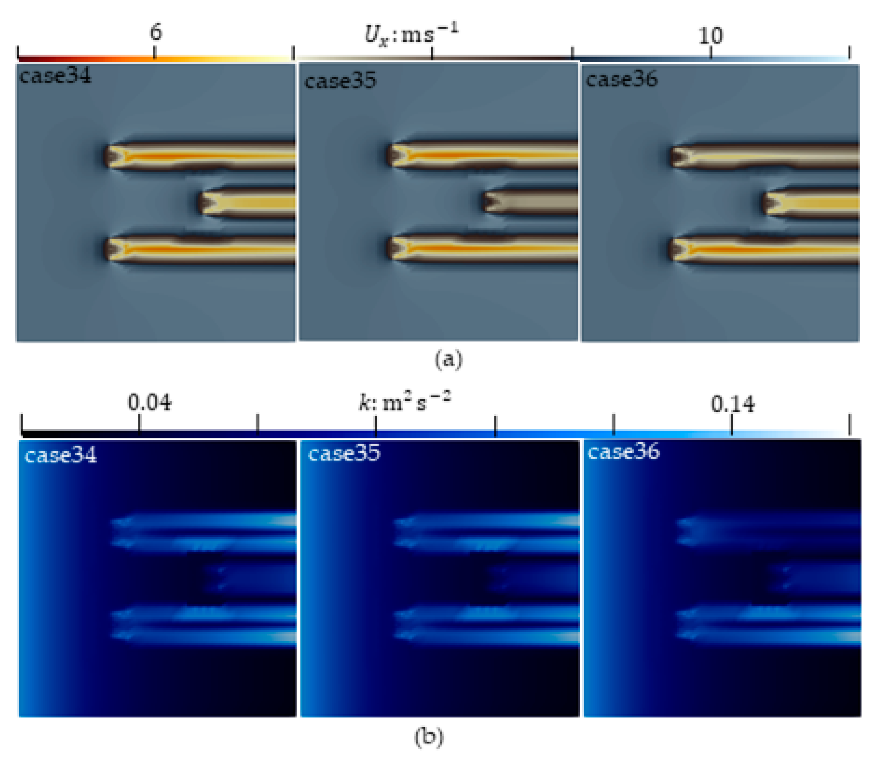
3.2.3. Three Staggered HAWTs

Power coefficients for the three staggered HAWTs are shown in Table 6. Combined with the previous calculation results, it can be seen that: The power of each HAWT in Case (32) is basically equal with d 1 = 4 D and d 2 = 4 D ; As the distance d 1 = 1 D and d 2 = 1.2 D between the front-rea1r and left-right HAWTs increase to d 1 = 4 D and d 2 = 4 D , the total power coefficient increases from 1.087 to 1.272. Comparing case (33) with case (25), after placing a HAWT in the center back of the two left–right HAWTs with d 2 = 1.2 D , the total power of the front two left–right HAWTs decreases from 0.804 for case (25) to 0.776 for case (33). Comparing case (32) with case (17) and case (27), it can be seen that when the left and right spacing is d 1 = 4 D , the power of each front left–right HAWTs is basically equal, and the power of the rear Rotor3 is equivalent to that of the front left and right HAWTs; However, when the two front–rear HAWTs rotate on the same axis, the power of the rear HAWT decreases to 70.1% of that of the front HAWT; This result to some extent indicates the superiority of a staggered arrangement of wind farm HAWTs. To set TSR = 7 for the right HAWT, the distance d 1 = 4 D and d 2 = 4 D , and the rotating speed in the same value. If the rotating speed direction of Rotor3 is the same or opposite, we get case (34) or case (35). Only when the Rotor2 has the opposite rotating direction and other settings are the same, it is case (36). The axial velocity and turbulent kinetic energy of these three cases are shown in Figure 14. From the figure, it is apparent that, when the rotating speed directions of the three HAWTs are the same, the axial velocity has a significant decrease at the blade hub. When only one HAWT reverses, the wake flow of the reversed HAWT is blurry, and there will no longer be a significant decrease in axial velocity at the hub, such as the rear Rotor3 in case (35) and the left Rotor2 in case (36). Distributions of turbulent kinetic energy in the same rotating direction of three HAWTs in case (34) and in case (35) with only Rotor3 reversing are similar; when only the left Rotor2 reverses direction, turbulent kinetic energy at the wake of both Rotor3 and Rotor2 is comparable to that of case (34) and case (35), while turbulent kinetic energy at the wake of Rotor2 decreases.

3.3. HAWTs Arrays

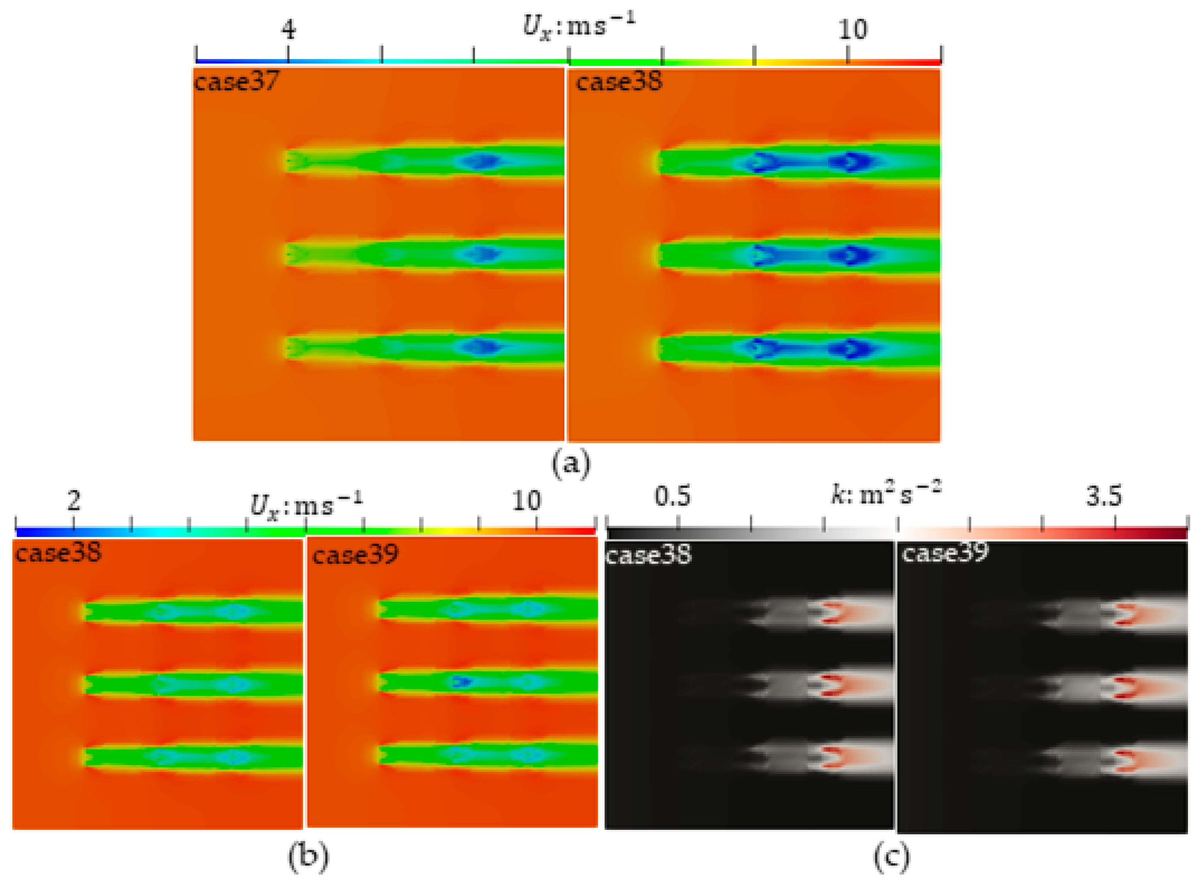
3.3.1. A Three-Rows and Three-Columns HAWTs Array

A three-rows and three-columns HAWTs array with uniform distances d 1 = 4 D and d 2 = 4 D is set. All HAWTs have the same rotating speed. Note case (37) with the first row HAWTs of TSR = 4, case (38) and case (39) with the first row HAWTs of TSR = 7, and case (39) has only the middle HAWT (Rotor5) turning in the opposite direction. Axial-velocity and turbulent-kinetic-energy field are shown in Figure 15, which shows that, as the TSR of the first row HAWTs increases, the overall wake velocity loss and region size increase, as shown in Figure 15a. Comparing case (37) with case (38), when TSR = 4, there is basically no low axial velocity component at the center of the first and second rows HAWTs wake. As TSR increases, an axial velocity component similar to the third row HAWTs wake appears at the second row HAWTs wake. Comparing case (38) with case (39), the turbulent kinetic energy region is basically the same, as shown in Figure 15c. A larger axial velocity loss in the wake of the middle HAWT (Rotor5) in case (39) can be observed, as shown in Figure 15b.

3.3.2. A One-Row and Three-Columns HAWTs Array with ABL

In order to consider the actual flow field of HAWTs arrays in the wind farm, a scene has been specially designed here, where a one-row and three-columns HAWTs array is placed in a mountainous area, as shown in Figure 16a. The mountain shape here is randomly generated, with the lowest point of the mountain being 100 m above sea level and the highest point of the mountain being 207.3 m above sea level. The atmospheric boundary layer model [29,30] is added. An inlet velocity profile is obtained from ground surface friction velocity, flow direction (positive direction of x -axis) and “vertical” direction. The lowest point of the ground and the surface roughness height are set respectively as z = 0 m and z 0 = 0.1 m. The reference speed at a height of 20 m above the ground is U r e f = 10 m/s. Axial velocity and turbulent kinetic energy fields are given in Figure 16b,c. We can derive from these that the axial velocity loss is greater in the closest rotor to the mountain surface (Rotor1) and the farthest from the mountain surface (Rotor2), as shown in Figure 16b, which indicates the importance of terrain on the influence of HAWTs wake flow. The axial velocity loss areas of the three HAWTs are similar. The turbulence kinetic energy caused by the HAWT farthest from the ground is the smallest, and due to different mountain terrain, turbulence kinetic energy in the wake of the three HAWTs shows different sizes, as shown in Figure 16c.

3.4. Sensitivity Analysis

In order to conduct an in-depth analysis of the performance of wind-turbine arrays with different arrangements for practical selection decisions, and for simplicity, here we only perform a sensitivity analysis on the two HAWTs arrangement to study the effect of power coefficients relative to different spacing between wind turbines in different directions. The results are shown in Figure 17. From the figure, it can be seen that in the direction of the wind, the distance d 1 between the front and rear HAWTs has a significant impact on the power of the rear HAWT. However, when d 1 > 6 D , there is basically no gain in HAWT power after increasing d 1 . The power of the upstream HAWT only slightly decreases with d 1 being too small or too large, and remains basically unchanged overall. In the crosswind direction, as the distance d 2 between the left and right HAWTs changes, the power changes of the left and right HAWTs are consistent, which is also in line with our usual intuition. At around d 2 = 2 D , whether it is a single HAWT power or two total power, there is a minimum value. When the left and right HAWTs do not collide, the total power will increase when d 2 < 2 D , and its increase rate is greater than when d 2 > 2 D .

4. Conclusions

This article reviews and studies six different numerical modeling methods for HAWTs. A series of numerical experiments were conducted on a commercial mesoscale Nordbank NTK 500/41 three-blade HAWT using different methods, including single-HAWT and multi-HAWTs flow fields. In the single-HAWT numerical experiment, DM and BEM-CFD methods were used, and also different blade cross-section airfoils were used, to explain why the BEM-CFD method was used in the calculation of HAWT array flow fields in large wind farms. In numerical experiments on multiple HAWTs, the BEM-CFD method was mainly used to study the flow field of HAWT arrays with different arrangements and the power obtained by the HAWTs, and some beneficial results were obtained. In line with the two main issues proposed in the first section of this article, here we only provide our two most important conclusions, accordingly:
  • The BEM-CFD method greatly improves the calculation speed within an accuracy range of thrust coefficients less than 2.5%, making it very suitable for the calculation of large wind farm HAWT arrays; By using the results of uniform loading in the BEM-CFD method, the HAWT can be subjected to any desired non-uniform loading, which is very meaningful for optimizing the design of the HAWT.
  • For regular HAWT arrays, it is reasonable to choose a 6 D spacing in the wind direction and a 4 D spacing in the crosswind direction for simplicity in practice. In order to improve the total power acquisition of a large wind farm HAWT array, we can adopt irregular HAWT array arrangements. Among them, this irregularity includes: the rotation direction of the HAWT arrays can be inconsistent, the size of the HAWTs and the cross-sectional airfoil of the HAWT blades cannot be the same, and so on. Further research is needed on which of these irregularly arranged HAWT arrays or regular HAWT arrays with real-time control systems has the lower cost.
Note that our research also has certain limitations, such as our numerical experiments being conducted under the assumption of an incompressible flow field. The wind always follows one direction without considering the real-time control system of the HAWT, and the HAWT does not perform any yaw or tilt movements. Consideration of the complexity of real atmosphere is also insufficient. However, these limitations do not affect our intention to answer the two main questions that this article aims to explore.

Author Contributions

Conceptualization, L.Y. and X.Z.; Methodology, L.Y. and X.Z.; Software, L.Y.; Validation, L.Y.; Formal analysis, L.Y.; Investigation, L.Y.; Resources, L.Y.; Data curation, L.Y. and E.G.; Writing—original draft, L.Y.; Writing—review & editing, X.Z. and E.G.; Supervision, X.Z. All authors have read and agreed to the published version of the manuscript.

Funding

This research was funded by National Key Research and Development Program of China, grant number No.2020YFB1506701, National Natural Science Foundation of China, grant numbers Nos.51739001/51879051, Open Fund of the Key Laboratory of Far-shore Wind Power Technology of Zhejiang Province in China, grant number ZOE20200007, Natural Science Foundation of Heilongjiang Province in China, grant number LH2020E071, Guangdong Branch of National Engineering Research Center for Offshore Wind power in China, grant number 2019B090904005.

Institutional Review Board Statement

Not applicable.

Informed Consent Statement

Not applicable.

Data Availability Statement

Not applicable.

Conflicts of Interest

The authors declare no conflict of interest.

Abbreviations

The following abbreviations are used in this article, which are given according to their order of appearance:
HAWThorizontal-axis wind-turbine
AManalytical method
VMvortex-lattice or particle method
PMpanel method
BEMblade element momentum method
GAMgeneralized actuator method
DMdirect modeling method
CFDcomputational fluid dynamics
TSRtip-speed ratio
ABLatmospheric boundary layer
ReReynolds number
DNSdirect numerical simulation
ADactuator disk method
ASactuator surface method
ALactuator line method
RANSReynolds average Navier–Stokes equation
LESlarge eddy simulation
PDpermeable disk
MaMach number
BCsboundary conditions
ICsinitial conditions
PISOalgorithm of pressure-implicit splitting-operators
GAAMgeometric aggregated algebraic multi grid method
SIMPLEsemi-implicit method for pressure linked equations

References

  1. Gyimah, R.R. The hot zones are cities: Methodological outcomes and synthesis of surface urban heat island effect in Africa. Cogent Soc. Sci. 2023, 9, 2165651. [Google Scholar] [CrossRef]
  2. Huang, C.H.; Tsai, H.H.; Chen, C.H. Observation of the vertical structure of atmospheric boundary layer in subtropical UHI by radiosonde. Geocarto Int. 2023, 38, 2208553. [Google Scholar] [CrossRef]
  3. Global Wind Report 2021. Available online: https://gwec.net/GWEC (accessed on 1 September 2022).
  4. Mao, X.; Sørensen, J.N. Far-wake meandering induced by atmospheric eddies in flow past a wind turbine. J. Fluid Mech. 2018, 846, 190–209. [Google Scholar] [CrossRef]
  5. Tummala, A.; Velamati, R.K.; Sinha, D.K.; Indraja, V.; Krishna, V.H. A review on small scale wind turbines. Renew. Sustain. Energy Rev. 2016, 56, 1351–1371. [Google Scholar] [CrossRef]
  6. Wang, C.; Prinn, R.G. Potential climatic impacts and reliability of very large-scale wind farms. Atmos. Chem. Phys. 2010, 10, 2053–2061. [Google Scholar] [CrossRef]
  7. Fiedler, B.H.; Bukovsky, M.S. The effect of a giant wind farm on precipitation in a regional climate model. Environ. Res. Lett. 2011, 6, 045101. [Google Scholar] [CrossRef]
  8. Ruan, Z.; Lu, X.; Wang, S.; Xing, J.; Wang, W.; Chen, D.; Nielsen, C.P.; Luo, Y.; He, K.; Hao, J. Impacts of large-scale deployment of mountainous wind farms on wintertime regional air quality in the Beijing-Tian-Hebei area. Atmos. Environ. 2022, 278, 119074. [Google Scholar] [CrossRef]
  9. Fröhlich, J.; Kuerten, H.; Geurts, B.J.; Armenio, V. Direct and Large-Eddy Simulation IX; Springer International Publishing: Cham, Switzerland, 2015. [Google Scholar] [CrossRef]
  10. Dasari, T.; Wu, Y.; Liu, Y.; Hong, J. Near-wake behaviour of a utility-scale wind turbine. J. Fluid Mech. 2019, 859, 204–246. [Google Scholar] [CrossRef]
  11. Hansen, M.O.L.; Sorensen, J.N.; Voutsinas, S.; Sørensen, N.; Madsen, H.A. State of the art in wind turbine aerodynamics and aeroelasticity. Prog. Aerosp. Sci. 2006, 42, 285–330. [Google Scholar] [CrossRef]
  12. Joshi, H.; Thomas, P. Review of vortex lattice method for supersonic aircraft design. Aeronaut. J. 2023, 25, 1–35. [Google Scholar] [CrossRef]
  13. Chen, C.W.; Peng, N. Prediction and analysis of 3D hydrofoil and propeller under potential flow using panel method. MATEC Web Conf. 2016, 77, 01013. [Google Scholar] [CrossRef]
  14. Amoretti, T.; Huet, F.; Garambois, P.; Roucoules, L. Configurable dual rotor wind turbine model based on BEM method: Co-rotating and counter-rotating comparison. Energy Convers. Manag. 2023, 293, 117464. [Google Scholar] [CrossRef]
  15. Fan, S.L.; Liu, Z.Q. Proposal of fully-coupled actuated disk model for wind turbine operation modeling in turbulent flow field due to complex topography. Energy 2023, 284, 128509. [Google Scholar] [CrossRef]
  16. Kim, T.; Oh, S.; Yee, K. Improved actuator surface method for wind turbine application. Renew. Energy 2015, 76, 16–26. [Google Scholar] [CrossRef]
  17. Yu, Z.Y.; Zheng, X.; Ma, Q.W. Study on actuator line modeling of two NREL 5-MW wind turbine wakes. Appl. Sci. 2018, 8, 434. [Google Scholar] [CrossRef]
  18. Kleine, V.G.; Hanifi, A.; Henningson, D.S. Non-iterative vortex-based smearing correction for the actuator line method. J. Fluid Mech. 2023, 961, A29. [Google Scholar] [CrossRef]
  19. Min, B. Introduction to Nordbank NTK 300kW Wind Turbine Generator. Available online: http://www.cqvip.com (accessed on 1 September 2022).
  20. Moukalled, F.; Mangani, L.; Darwish, M. The Finite Volume Method in Computational Fluid Dynamics; Springer International Publishing: Cham, Switzerland, 2016. [Google Scholar]
  21. Hansen, M.O.L. Aerodynamics of Wind Turbines; Library of Congress Cataloging-in-Publication Data: Washington, DC, USA, 2015. [Google Scholar]
  22. Ferrer, E.; Montlaur, A. CFD for wind and tidal offshore turbines. In Springer Tracts in Mechanical Engineering; Springer International Publishing: Cham, Switzerland, 2015. [Google Scholar] [CrossRef]
  23. Glauert, H. Aerodynamic Theory: Airplane Propellers; Springer: New York, NY, USA, 1935; Volume 4, pp. 169–360. [Google Scholar]
  24. Burton, T.; Jenkins, N.; Sharpe, D.; Bossanyi, E. Wind Energy Handbook; John Wiley and Sons, Ltd.: Chichester, UK, 2011. [Google Scholar]
  25. Peña, A.; Mirocha, J.D.; Laan, M.P.V.D. Evaluation of the fitch wind-farm wake parameterization with large-eddy simulations of wakes using the weather research and forecasting model. Am. Meteorol. Soc. 2022, 150, 3051–3064. [Google Scholar] [CrossRef]
  26. Calaf, M.; Meneveau, C.; Meyers, J. Large eddy simulation study of fully developed wind-turbine array boundary layers. Phys. Fluids 2010, 22, 015110. [Google Scholar] [CrossRef]
  27. Shen, W.Z.; Sorensen, J.N.; Mikkelsen, R. Tip loss correction for actuator/Navier-Stokes computations. J. Sol. Energy Eng. 2005, 127, 209–213. [Google Scholar] [CrossRef]
  28. Ma, Y.; Archer, C.L.; Vasel-Be-Hagh, A. The Jensen wind farm parameterization. Wind Energy Sci. 2022, 7, 2407–2431. [Google Scholar] [CrossRef]
  29. Hargreaves, D.M.; Wright, N.G. On the use of the k-epsilon model in commercial CFD software to model the neutral atmospheric boundary layer. J. Wind Eng. Ind. Aerodyn. 2007, 95, 355–369. [Google Scholar] [CrossRef]
  30. Deremble, B.; Wienders, N.; Dewar, W.K. CheapAML: A simple, atmospheric boundary layer model for use in ocean-only model calculations. Am. Meteorol. Soc. 2013, 141, 809–821. [Google Scholar] [CrossRef]
Figure 1. Top 10 countries with installed capacity and their proportion in the world as of 2020.
Wind 03 00026 g001
Figure 2. Wind turbine blade-modeling.
Wind 03 00026 g002
Figure 3. Geometry description of wind turbine: (a) Relative chord length and twist angle distribution; (b) Two NACA six-digit laminar airfoils; (c) Lift coefficient (black solid line represents NACA63-210 airfoil at Re = 10 6 ; orange solid line represents Re = 5 × 10 5 , blue solid line represents Re = 5 × 10 4 ; and red solid line represents NACA63-412 airfoil at Re = 10 6 ); (d) Drag coefficient.
Wind 03 00026 g003
Figure 4. Schematic diagram of one-dimensional momentum theory: (a) Streamlines past the rotor; (b) Velocity and pressure distribution; (c) Control volume.
Wind 03 00026 g004
Figure 5. Influence of rotor rotation and optimal power output. (a) Relative velocity upstream and downstream of airfoil; (b) The local loads on a blade and velocities at the rotor plane; (c) The numerical relationships between a , a and x ; (d) Optimal power output of rotors with different TSRs.
Wind 03 00026 g005
Figure 6. BEM-CFD method and analytical model. (a) Flow chart of BEM-CFD method; (b) Non-uniform loading; (c) Jensen wake model.
Wind 03 00026 g006aWind 03 00026 g006b
Figure 7. Description of numerical calculation domain with d 0 = 4 D : (a) Single HAWT (top view); (b) Two front-rear HAWTs; (c) Two left-right HAWTs; (d) Three staggered HAWTs; (e) A 3-rows and 3-columns HAWTs array.
Wind 03 00026 g007
Figure 8. Overall meshing: (a) Meshing for DM method; (b) Meshing for BEM-CFD method.
Wind 03 00026 g008
Figure 9. Wind turbine power: (a) Comparison of calculated and measured power (the red solid line is the measured result, the black triangle dots are the results of the modified BEM method by Glauert and Prandtl, the hollow circle dots are the results of our BEM-CFD methods with T S R = 4–12 integers from the bottom to the top, and the yellow solid circle dot represents the result of T S R = 6); (b) Variation of power-coefficient with tip-speed-ratio (blue line is the measured value, orange circle dots are the results of our cases (6–14) from left to right, black circle dot is the results of a refinement meshing); (c) Variation of power-coefficient with reciprocal of tip-speed-ratio.
Wind 03 00026 g009
Figure 10. Comparison of results between DM method and BEM-CFD method: (a) Axial velocity; (b) Turbulent kinetic energy.
Wind 03 00026 g010
Figure 11. Comparison of flow fields under different TSRs: (ac) Velocity components; (d) Pressure; (e) ω ; (f) Turbulent viscosity; (g) Turbulent kinetic energy; (h,i) Case (6) close-up ν t and k .
Wind 03 00026 g011
Figure 12. Comparison of the same and opposite rotating speeds of two front–rear HAWTs: (a) Axial velocity; (b) Turbulent kinetic energy; (c,d) Results with same setting as case (21,22) except d 1 = 1 D .
Wind 03 00026 g012
Figure 13. Comparison of the same and opposite rotating speeds of two left–right HAWTs: (a) Axial velocity; (b) Turbulent kinetic energy; (c,d) Results with same setting as case (28,29) except d 2 = 4 D ; (e) Close-up turbulence kinetic energy of case (30,31).
Wind 03 00026 g013
Figure 14. Comparison of three staggered HAWTs with the same and only one HAWT with opposite rotational speeds: (a) Axial velocity; (b) Turbulent kinetic energy.
Wind 03 00026 g014
Figure 15. Flow field of A 3-rows and 3-columns HAWTs array: (a) Axial velocity comparison with different TSRs; (b) Axial velocity comparison of case (38) and case (39); (c) Turbulent kinetic energy comparison of case (38) and case (39).
Wind 03 00026 g015
Figure 16. A wind-turbine array in the atmospheric boundary layer: (a) Specially designed scenarios (the lower-right corner is a screenshot in the HAWTs rotor plane); (b) Axial velocity; (c) Turbulent kinetic energy.
Wind 03 00026 g016
Figure 17. A sensitivity analysis of two HAWTs arrangements: (a) At front-and-rear; (b) At left-and-right.
Wind 03 00026 g017
Table 1. Forty cases of numerical experiments.
Number of HAWTsCasesDomain
singlecase (1–14)cylinder
two at front and rearcase (15–24)cylinder
two at left and rightcase (25–31)block
three staggeredcase (32–36)block
3-rows and 3-columnscase (37–39)block
1-row and 3-columns 1case (40)block
1 With ABL.
Table 2. Initial and boundary conditions.
BCs U : m/s p : m2 · s−2 k : m2 · s−2 ε : m2 · s−3 ω : s−1 ν t : m2 · s−1
Inletfixed valuezero gradientfixed valuefixed valuefixed valuecalculated
Outletinlet outletfixed valueinlet outletinlet outletinlet outletcalculated
Wallsno slipzero gradientwall functionwall function-wall function
Othersslipslipslip-slipslip
Note: Initial velocity of the flow field is set to (10 0 0) m/s for all cases except for specific instructions.
Table 3. Thrust coefficient and calculation cost.
Case C T Relative ErrorCostMethod
(1)0.005--DM
(2) 10.823ReferencevalueDM
(3) 20.767--DM
(4) 10.8361.8%5042BEM-CFD
(5) 10.8402.1%90BEM-CFD
1 With airfoil NACA63-412. 2 With airfoil NACA63-210.
Table 4. Two front-rear HAWTs.
Case d 1 Rotor1-Front C P Rotor2-Rear C P Rotor2/Rotor1
(15) 1 D 0.4430.26660.1%
(16) 2 D 0.4470.30067.2%
(17) 4 D 0.4490.31570.1%
(18) 6 D 0.4520.37983.9%
(19) 8 D 0.4470.38986.9%
(20) 10 D 0.4450.39388.4%
Table 5. Two left–right HAWTs.
Cased2Rotor1-Right C P Rotor2-Left C P Rotor2 + Rotor1
(25) 1.2 D 0.4110.3930.804
(26) 2 D 0.3540.3650.719
(27) 4 D 0.4220.4280.850
Table 6. Staggered three HAWTs.
Case d 1 d 2 Rotor1-Right C P Rotor2-Left C P Rotor3-Rear C P Rotor (1 + 2 + 3) C P
(32) 4 D 4 D 0.4200.4280.4241.272
(33) 1 D 1.2 D 0.3940.3820.3111.087
Disclaimer/Publisher’s Note: The statements, opinions and data contained in all publications are solely those of the individual author(s) and contributor(s) and not of MDPI and/or the editor(s). MDPI and/or the editor(s) disclaim responsibility for any injury to people or property resulting from any ideas, methods, instructions or products referred to in the content.

