Knowledge-Based Image Analysis: Bayesian Evidences Enable the Comparison of Different Image Segmentation Pipelines ^†

Abstract

The analysis and evaluation of microscopic image data is essential in life sciences. Increasing temporal and spatial digital image resolution and the size of data sets promotes the necessity of automated image analysis. Previously, our group proposed a Bayesian formalism that allows for converting the experimenter’s knowledge, in the form of a manually segmented image, into machine-readable probability distributions of the parameters of an image segmentation pipeline. This approach preserved the level of detail provided by expert knowledge and interobserver variability and has proven robust to a variety of recording qualities and imaging artifacts. In the present work, Bayesian evidences were used to compare different image processing pipelines. As an illustrative example, a microscopic phase contrast image of a wound healing assay and its manual segmentation by the experimenter (ground truth) are used. Six different variations of image segmentation pipelines are introduced. The aim was to find the image segmentation pipeline that is best to automatically segment the input image given the expert knowledge with respect to the principle of Occam’s razor to avoid unnecessary complexity and computation. While none of the introduced image segmentation pipelines fail completely, it is illustrated that assessing the quality of the image segmentation with the naked eye is not feasible. Bayesian evidence (and the intrinsically estimated uncertainty $\sigma$ of the image segmentation) is used to choose the best image processing pipeline for the given image. This work illustrates a proof of principle and is extendable to a diverse range of image segmentation problems.

1. Introduction

Identifying regions of interest in data sets of biological processes from microscopic imaging is of central interest in physiology and cell biology. Data sets might be recorded at high temporal and spatial resolution. Thus, the increase in data size prompts the need for automated image segmentation. However, this task is often performed manually by experimenters, who apply their expert knowledge to the data set. Knowledge-based analysis describes the concept of transferring expert knowledge into machine-readable data or a code to subsequently apply this to new data sets. Bayesian inference can be used for this purpose, where the expert knowledge is converted to posterior distributions of model parameters, as previously demonstrated by our group [1]. These parameters represent a variety of image features, such as brightness thresholds or smoothing kernel filter sizes of the applied image segmentation pipeline.

During discussions with members of the life science community on our previous work [1], the question of why certain image processing pipelines should be chosen over others arose. In the present work, we use Bayesian evidences to compare different pipelines for image segmentation. This allows for generating robust image segmentation pipelines without overfitting. The performances of these algorithms are illustrated with real-world problems, such as the analysis of the temporal cellular closure of a wound.

2. Materials and Methods

2.1. Data

Wound healing assays are commonly used to quantify collective cell motility over time. Cells are seeded in two compartments of a separating insert, resulting in two cell populations with a defined gap. After the removal of the insert, cells move into the cell-free gap area. While cell migration is recorded over time, one representative region of interest was selected on a single frame as an illustrative example in this work (see Figure 1).

2.2. Workflow

Data processing, as suggested in our previous work, [1] follows a three-step protocol:

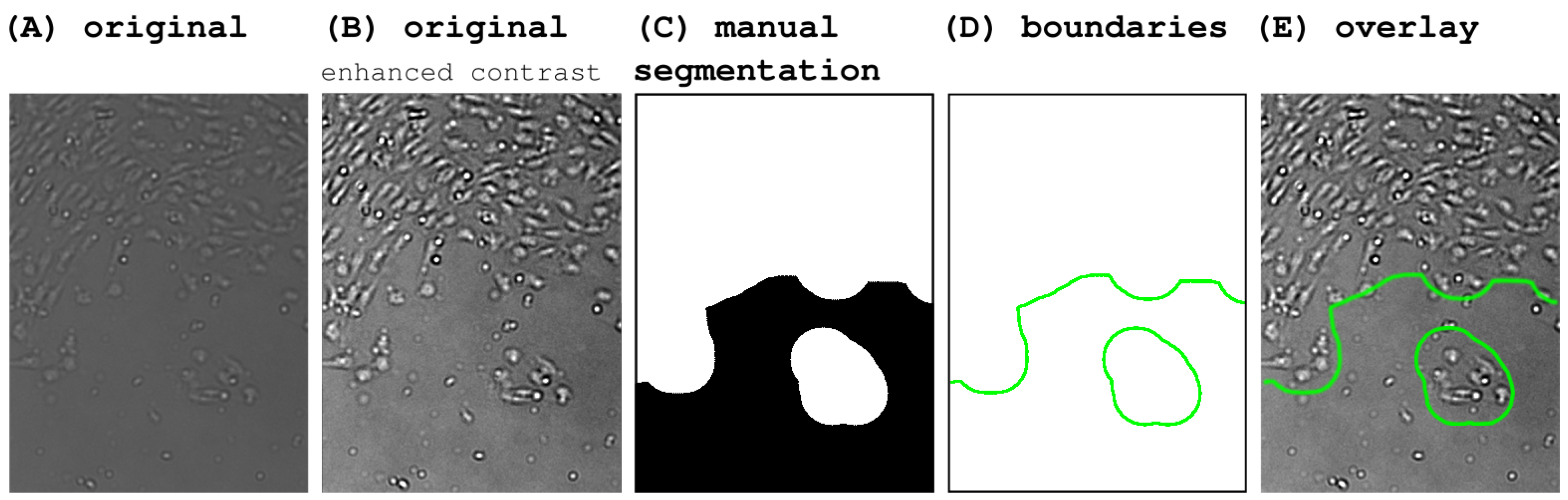
• User input: The experimenter manually marks regions with and without cells, resulting in a manually segmented image from the time series (see Figure 1).
• Bayesian parameter and evidence estimation: Bayesian inference is applied to different parameter-dependent image segmentation pipelines using the manually segmented image as input data. A metric distance is applied to measure the difference between the manually segmented image and the pipeline-generated images (see below). During parameter estimation, the distance between the manually and the pipeline-segmented image will be optimized, resulting in the conversion of the expert knowledge to machine-readable posterior distributions of parameters.
• Application: Based on the estimated Bayesian evidences as quality criteria of the image segmentation pipelines, one image segmentation pipeline can be chosen, and the optimized parameter set can be applied to the entire image series.

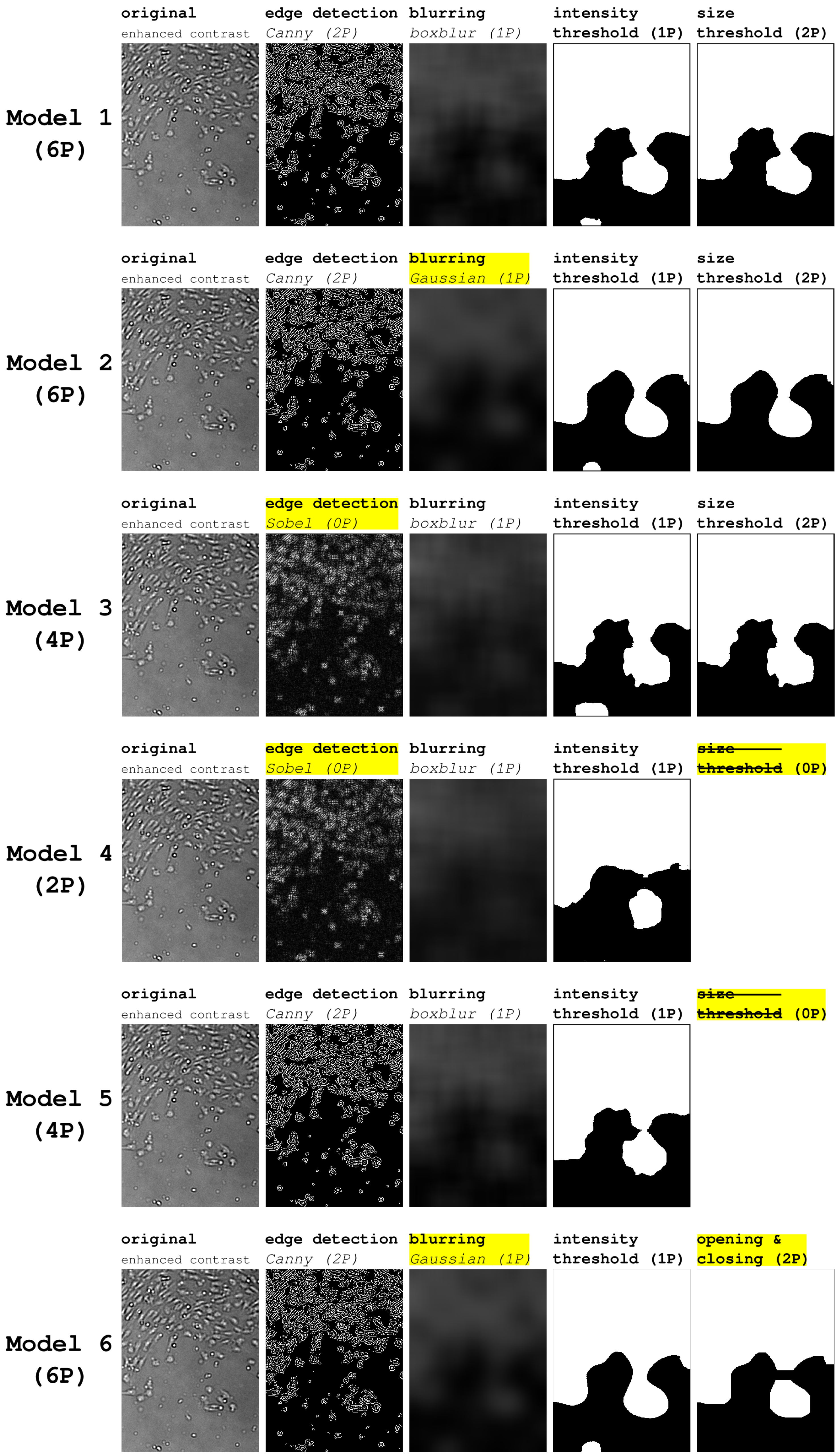
2.3. Image Segmentation Pipelines

In our previous work, we used an image segmentation pipeline consisting of a sequence of different filters [2,3]. A similar approach with manual adaptation of parameters was described previously [4]. Figure 2 illustrates the different image segmentation pipelines used throughout this work. All image segmentation pipelines were implemented in the Python programming language using scipy and opencv libraries [5,6].

Model 1

consists of the following elements: A canny edge detection with two free parameters is performed under the assumption that cell-covered areas have more edges than cell-free areas. Consecutively, the resulting image is blurred by using a box blur filter to merge the previously found edges into an area. An intensity threshold is used to obtain a binary image. Furthermore, on the binary image, two size thresholds for contiguous small areas of black or white pixels are applied under the assumption that, most likely, small areas represent artifacts. Model 1 has 6 free parameters.

In the following, the variations of Models 2–6 in comparison with Model 1 are highlighted.

Model 2

uses a Gaussian filter instead of the box blur. While the Gaussian filter is computationally more expensive than the box blur, it is assumed to better reproduce the natural curves of the cells in the image than the rectangular box blur. Model 2 has 6 free parameters.

Model 3

uses the Sobel filter with a fixed parameter set (of kernel size 3 pixels) instead of the canny edge detection. The Sobel filter is a less computational expensive edge detection algorithm and a more general approach. Model 3 has 4 free parameters.

Model 4

also uses a Sobel filter. Further, Model 4 does not apply size thresholds for small areas of black or white pixels. Thus, it is the least computational expensive model in this series, but does not correct for any artifacts. Model 4 has 2 free parameters.

Model 5

is the same as Model 1 without size thresholds and, therefore, does also not correct for small artifacts. Model 5 has 4 free parameters.

Model 6

is similar to Model 2 as it uses Gaussian blurring, but instead of size thresholds, it applies opening and closing image filters, which are commonly used to filter out small regions. Model 6 has 6 free parameters.

2.4. Distance Metrics

To quantify the distance between the manually segmented and the pipeline-generated images, we focused on the border between the black and the white pixels since it condenses the most important information of the binary image. For two boundaries, we performed a pixelwise distance to the closest point operation [7]. We defined that the pixelwise distance to the closest point is always measured from the longer to the shorter boundary to make the distance metric. Further, the distance from the shorter to the longer boundary would result in a convergence of the length of the pipeline-generated image towards 0.

Thus, the distance between every pixel position $a_i$ of the longer boundary A (of length m) and the shorter boundary B (of length n) is noted as follows:

$$d_i(a_i,B{P}_B)=\underset{j=1\dots n}{min}\left|\right|b_j-a_i\left|\right|$$

(1)

where $\left|\right|x-y\left|\right|$ denotes the Euclidean distance between two points and $B{P}_B$ denotes all n points of the boundary B. We call the ensemble of all distances the boundary distance $BD$ with $\{d_1\dots d_m\}$.

It is noteworthy that $BD$ is a spatial metric, which is different from other commonly used pixel-based metrics. Therefore, it not only is more intuitive for intended users, such as physiologists, but also allows for assessing the spatial uncertainty from the Bayesian inference (see below).

2.5. Bayesian Inference

We used Bayesian inference to select the optimal image segmentation pipeline and consecutively perform a parameter estimation of the parameter set $\mathit{\theta }$ of the selected image segmentation pipeline. An optimal image segmentation pipeline in the Bayesian logic requires sufficient free parameters to cover the characteristics of the image, but does not overfit using too many parameters (principle of Occam’s razor; see below).

Derived from the general Bayes’ theorem

$$P\left(A|B\right)=\frac{P\left(B\right|A)\times P(A)}{P\left(B\right)}$$

(2)

we want to assess the conditional probability $P\left(\mathit{\theta }\right|K)$ of the parameter set $\mathit{\theta }$ given the expert knowledge K. We choose the Bayesian a priori probability $P\left(\mathit{\theta }\right)$ of the parameter set $\mathit{\theta }$ to be constant for all parameters as they represent spatial or intensity dimensions. The term $P\left(K\right)$ corresponds to the Bayesian evidence.

$$P\left(\mathit{\theta }|K\right)=\frac{P\left(K\right|\mathit{\theta })\times P(\mathit{\theta })}{P\left(K\right)}$$

(3)

The term $P\left(K\right|\mathit{\theta })$ represents the Bayesian likelihood (LH) and describes the similarity between the manually segmented image using the expert knowledge K and a pipeline-generated image using a parameter set $\mathit{\theta }$. Under the assumption of a Gaussian distributed uncertainty $\sigma$ of the boundary distance $BD=\{d_1\dots d_m\}$ between the manually segmented and the pipeline-segmented image, we denote the likelihood as

$$LH\left(K|\mathit{\theta }\right)=\prod _{i=1}^m\frac{1}{\sqrt{2\pi {\sigma }^2}}\times exp\left(-\frac{1}{2}\frac{d_i^2}{{\sigma }^2}\right)$$

(4)

Model selection will be performed based on the principle of Occam’s razor, which avoids unnecessary and unjustified complexity. If large areas of the parameter space have a high likelihood, the Bayesian evidence $P\left(K\right)$ has a higher value compared with parameter-likelihood spaces with large areas of low likelihood [8]. This can be paraphrased more simple as Bayesian evidence is high if the ratio of high likelihood to parameter space given by the model is justified. Thus, Bayesian evidence is taking the complexity of the models into account during model evaluation and is therefore used for model selection. For computational ease, the logarithmic evidence $ln\left(Z\right)$ will be used throughout this work.

2.6. Numerical Implementation

We used the multinested sampling algorithm [8,9,10] in its Python implementation [11]. This approach can be summarized in a simplified way as follows: The prior-likelihood space is scattered with a cloud of a random set of live points. For each live point, the likelihood is evaluated. Once all likelihoods of all live points in the cloud are evaluated, the one with the lowest likelihood is eliminated and replaced by a new random point with a higher likelihood. This replacement is performed iteratively. During the iteration process, the evidence can be calculated as the weighted sum of the sorted likelihoods.

We want to investigate whether the number of live points is critical to ensure that the prior likelihood space is scanned correctly (see Section 3.1).

3. Results

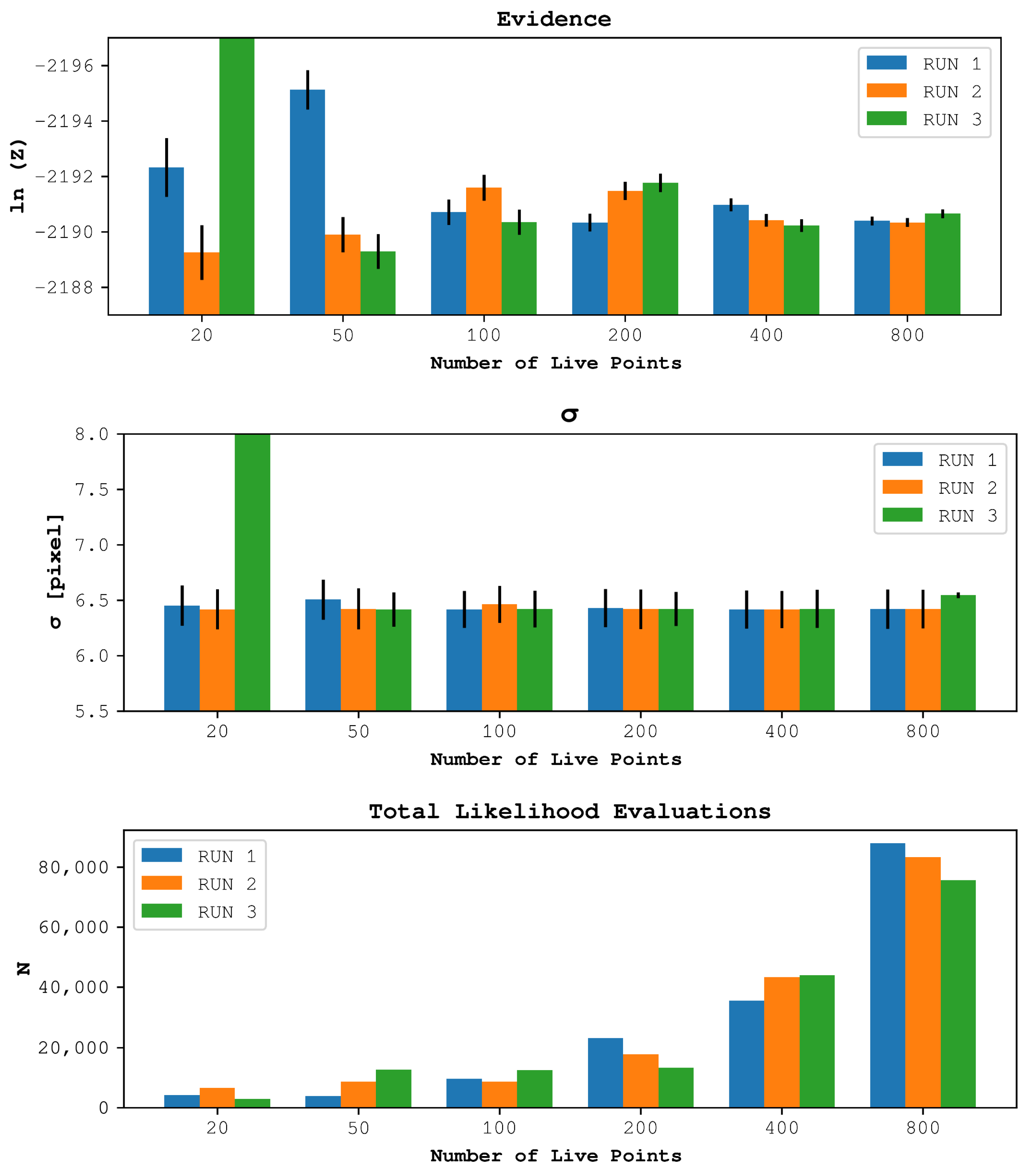
3.1. Determining the Necessary Number of Live Points

As explained above, the number of live points is critical for a sufficient sampling of the prior-likelihood space. Here, we applied the introduced formalism with different numbers of live points (20, 50, 100, 200, 400, 800) using Model 1. For each number of live points, Bayesian inference was applied three times independently. Consecutively, the estimated evidence, the estimated uncertainty $\sigma$, and the total number of likelihood evaluations during the iterative process were evaluated.

Results are shown in Figure 3: For 100 live points and above, the estimated logarithmic evidence $ln\left(Z\right)$ and the estimated uncertainty $\sigma$ remain stable. Thus, 100 live points were chosen throughout this work as they represent the optimized balance between computational workload and stability.

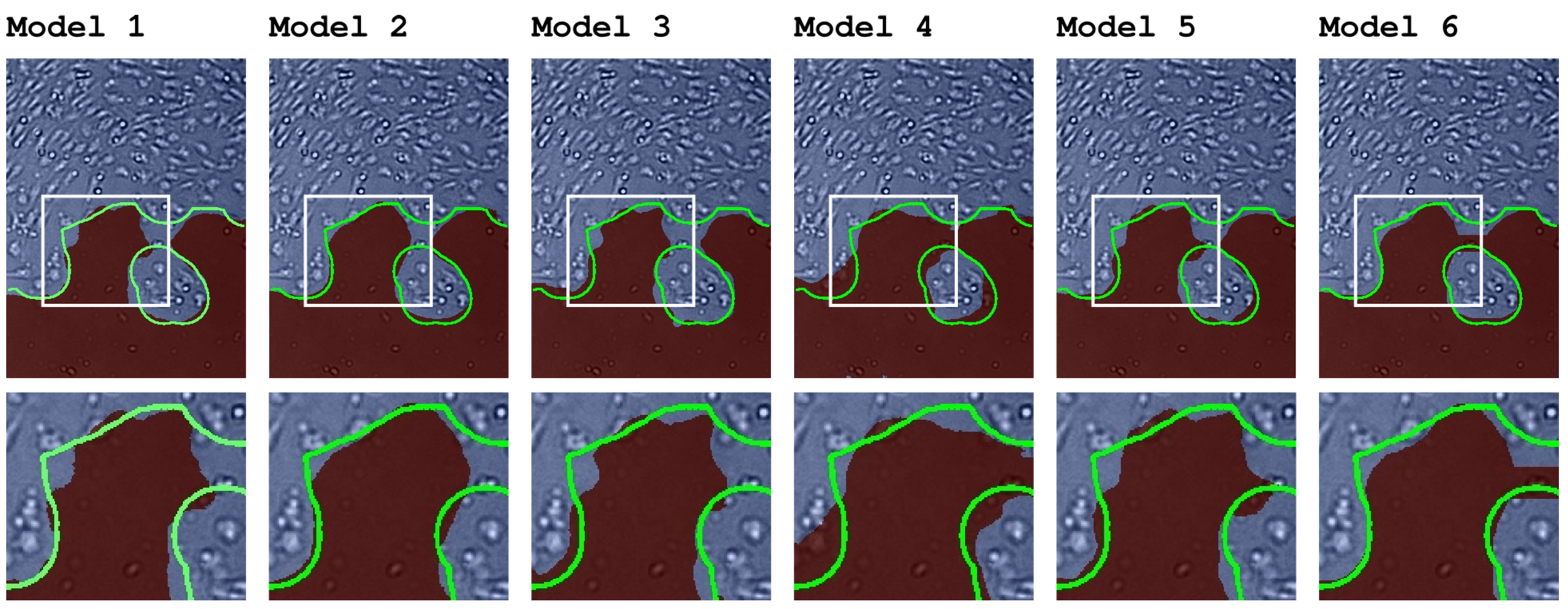
3.2. Image Segmentation Using the Estimated Posterior Parameters

Using Bayesian inference, we obtained the posterior distributions for parameter sets of Models 1–6. Consecutively, these posteriors were applied to obtain pipeline-generated images (see Figure 4, red and blue). At first sight, small differences in the segmentation of Models 1–6 became obvious. However, with the naked eye, it is infeasible to tell which algorithm is closest to the manually segmented image (see Figure 4, green). Please note that, for example, Models 4 and 6 are the only two models that fully surround the small island of cells in the lower center right of the original figure—as it was suggested by the manually segmented image. Furthermore, it seems impossible to decide which algorithm to select over the others only by looking at Figure 4.

3.3. Choosing the Image Segmentation Pipeline

Bayesian inference allows for choosing an image segmentation pipeline based on the Bayesian evidence, which is the probability that the given pipeline is capable of recreating the expert knowledge. Thus, the image segmentation with the highest Bayesian evidence should be chosen. According to

Table 1. Comparison of the different models based on Bayesian evidence (best results per column are marked in bold font).

	ln(Z)	$\mathbf{\sigma }$[pxl]	Calc. Time *
Model 1	$-\pm 0.5$	$6.40\pm 0.16$	02 min 59 s
Model 2	$-\mathbf{2098}.\mathbf{4}\pm \mathbf{0}.\mathbf{5}$	$\mathbf{5}.\mathbf{62}\pm \mathbf{0}.\mathbf{14}$	11 min 15 s
Model 3	$-2299.1\pm 0.4$	$7.48\pm 0.21$	01 min 11 s
Model 4	$-2559.5\pm 0.4$	$11.40\pm 0.34$	00 min 20 s
Model 5	$-2256.1\pm 0.5$	$7.09\pm 0.19$	01 min 03 s
Model 6	$-2112.2\pm 0.5$	$5.70\pm 0.15$	27 min 23 s

* Processor: i5-2520M CPU @ 2.50 GHz.

, Model 2 has the highest Bayesian evidence. Additionally, Model 2 shows the lowest uncertainty $\sigma$.

4. Discussion

While multiple image segmentation implementations focus on Bayesian decision trees for pixel-based classification [12], our group previously demonstrated the usage of Bayesian inference to perform a parameter estimation for a pre-setup imaging pipeline based on the segmentation of an input image, which is trained with expert knowledge. A possible advantage of this approach might consist of more consistently taking into account spatial correlations such as textures within image data than pixel-based Bayesian decision trees. Contrary to pixel-based classification, this approach uses a metric distance of boundaries of conjoined regions, which is more intuitive than pixel-based uncertainties in the perception and processing. This approach enables the logically consistent handling of Bayesian uncertainties of segmentation boundaries.

Our approach enables experimenters with little knowledge in computer science to manually segment one image of an image series and then use this expert knowledge to automatically choose the best image segmentation pipeline from a collection of tested pipelines with an optimized parameter set. In this work, we were able to demonstrate that (I) the needed number of live points can be assessed in a simple straightforward approach. However, it is worth mentioning that other implementations of nested sampling have the ability to correct the number of live points on the run [13]. (II) Objectively assessing the quality of pipeline-generated images is infeasible with the naked eye. (III) Bayesian evidence logically consistently enables the systematic selection of the best image segmentation pipeline among those tested.

As a future prospect, the developed technique can be further applied to other segmentation problems, such as time lapse series or 3D volume data.

References

1. Moskopp, M.L.; Deussen, A.; Dieterich, P. Bayesian inference for the automated adjustment of an image segmentation pipeline—A modular approach applied to wound healing assays. Knowl.-Based Syst. 2019, 173, 52–61. [Google Scholar] [CrossRef]
2. Canny, J. A Computational Approach to Edge Detection. IEEE Trans. Pattern Anal. Mach. Intell. 1986, PAMI-8, 679–698. [Google Scholar] [CrossRef]
3. Burger, W.; Burge, M.J. Digitale Bildverarbeitung: Eine Einführung mit Java und ImageJ; mit 16 Tabellen; eXamen.press; Springer: Berlin/Heidelberg, Germany, 2005. [Google Scholar]
4. Jonkman, J.E.N.; Cathcart, J.A.; Xu, F.; Bartolini, M.E.; Amon, J.E.; Stevens, K.M.; Colarusso, P. An introduction to the wound healing assay using live-cell microscopy. Cell Adhes. Migr. 2014, 8, 440–451. [Google Scholar] [CrossRef] [PubMed]
5. Virtanen, P.; Gommers, R.; Oliphant, T.E.; Haberland, M.; Reddy, T.; Cournapeau, D.; Burovski, E.; Peterson, P.; Weckesser, W.; Bright, J.; et al. SciPy 1.0: Fundamental algorithms for scientific computing in Python. Nat. Methods 2020, 17, 261–272. [Google Scholar] [CrossRef] [PubMed]
6. The OpenCV Reference Manual; Manual, Edition: 2.4.13.7; OpenCV: Palo Alto, CA, USA, 2014.
7. Chalana, V.; Kim, Y. A methodology for evaluation of boundary detection algorithms on medical images. IEEE Trans. Med. Imaging 1997, 16, 642–652. [Google Scholar] [CrossRef] [PubMed]
8. Feroz, F.; Hobson, M.P. Multimodal nested sampling: An efficient and robust alternative to Markov Chain Monte Carlo methods for astronomical data analyses: Multimodal nested sampling. Mon. Not. R. Astron. Soc. 2008, 384, 449–463. [Google Scholar] [CrossRef]
9. Skilling, J. Nested sampling for general Bayesian computation. Bayesian Anal. 2006, 1, 833–859. [Google Scholar] [CrossRef]
10. Von Toussaint, U. Bayesian inference in physics. Rev. Mod. Phys. 2011, 83, 943–999. [Google Scholar] [CrossRef]
11. Buchner, J.; Georgakakis, A.; Nandra, K.; Hsu, L.; Rangel, C.; Brightman, M.; Merloni, A.; Salvato, M.; Donley, J.; Kocevski, D. X-ray spectral modelling of the AGN obscuring region in the CDFS: Bayesian model selection and catalogue. Astron. Astrophys. 2014, 564, A125. [Google Scholar] [CrossRef]
12. Arganda-Carreras, I.; Kaynig, V.; Rueden, C.; Eliceiri, K.W.; Schindelin, J.; Cardona, A.; Sebastian Seung, H. Trainable Weka Segmentation: A machine learning tool for microscopy pixel classification. Bioinformatics 2017, 33, 2424–2426. [Google Scholar] [CrossRef] [PubMed]
13. Buchner, J. UltraNest—A robust, general purpose Bayesian inference engine. J. Open Source Softw. 2021, 6, 3001. [Google Scholar] [CrossRef]
Figure 1. Image data and manual segmentation. (A) A typical region of interest on an image of a wound healing assay can be seen. (B) The same region of interest as in panel (A) is shown with enhanced contrast for illustrative purposes. (C) A manual image segmentation for a cell-free (black) and cell-covered (white) area is shown. (D) The boundary between the black and the white pixels of the manual segmentation is indicated by a green line. This boundary is essential for distances between manually segmented images and pipeline-segmented images (see below). (E) An overlay of the contrast-enhanced original image and the boundary is given for visual clarification.
Psf 09 00020 g001
Figure 2. Image segmentation pipelines. The image segmentation pipelines (Models 1–6) consist of a sequence of image filters and algorithms that depend on one (1P) or two (2P) parameters. Further, some algorithms are applied with a fixed set of parameters (0P), so that no free parameters were used during parameter estimation. Differences of the applied filters with respect to Model 1 are highlighted in yellow. The original image is displayed with enhanced contrast for illustrative purposes only—calculations and shown results are based on the native original image (see Figure 1A).
Psf 09 00020 g002
Figure 3. Evaluation of the necessary number of live points. This figure shows the results for estimated logarithmic evidence l n ( Z ) , estimated uncertainty σ , and the total number of likelihood evaluations (N) for three independent applications of the previously introduced formalism using either 20, 50, 100, 200, 400, or 800 live points. With 100 live points or more, the estimated evidences l n ( Z ) and estimated uncertainties σ remain stable. Of the tested values with stable results, 100 live points require the least likelihood evaluations and are therefore computationally the most effective. (Data are shown as mean and Bayesian uncertainty (error bars) of the posterior distribution. Each estimation was independently run three times to evaluate reproducibility. In RUN 3 with 20 live points, results are 3095.7 ± 1.2 for l n ( Z ) and 40.5 ± 0.1 p i x e l for σ ; both are off the charts. These extreme results indicate a failure due to very few live points. For illustrative purposes, they were not taken into consideration for the limits of the y-axes.)
Psf 09 00020 g003
Figure 4. Image segmentation for Models 1–6. After applying the above-introduced formalism, estimated posterior parameters were used to obtain one pipeline-segmented image for Models 1–6. These images are overlays of the original input image (see Figure 1A). The pipeline-generated image is superimposed with dark red indicating a cell-free area and blue indicating a cell-covered area. The green line represents the boundary between a cell-free and a cell-covered area in the manually segmented image (see Figure 1D). The white box shows a region of interest, which is magnified in the lower part of the figure to magnify the details.
Psf 09 00020 g004