Snowballing Nested Sampling ^†

Abstract

A new way to run nested sampling, combined with realistic MCMC proposals to generate new live points, is presented. Nested sampling is run with a fixed number of MCMC steps. Subsequently, snowballing nested sampling extends the run to more and more live points. This stabilizes the MCMC proposal of later MCMC proposals, and leads to pleasant properties, including that the number of live points and number of MCMC steps do not have to be calibrated, that the evidence and posterior approximation improve as more compute is added and can be diagnosed with convergence diagnostics from the MCMC community. Snowballing nested sampling converges to a “perfect” nested sampling run with an infinite number of MCMC steps.

1. Introduction

Nested sampling [1] is a popular [2] Monte Carlo algorithm for Bayesian inference, estimating the posterior distribution and the Bayesian evidence. A set of K live points are initially drawn from the prior, and their likelihoods are evaluated. In each iteration of the algorithm, the live point with the lowest likelihood is discarded and becomes a dead point. It is replaced with a new point sampled from the prior, under the constraint that the likelihood of the discarded point is exceeded. This likelihood-restricted prior sampling (LRPS) can be achieved in various ways (see Buchner [3] for an extensive review).

Skilling [1] originally proposed Markov Chain Monte Carlo (MCMC) random walk algorithms for the LRPS. This is still the most popular choice for high-dimensional problems, including slice sampling variants (e.g., [4]), recently compared for efficiency and reliability in [5]. Such algorithms start from a randomly chosen live point and make M transitions to yield the new live point. To avoid a collapse of the live point set, and sufficiently explore the likelihood-restricted prior, M has to be chosen large enough. However, as Salomone et al. [6] discusses, mild correlations between live points are acceptable. Thus, a suitably efficient LRPS algorithm has to be chosen by the user, as well as the size of the live points, K, which regulates the resolution of the sampling and the uncertainty on the outputs. Since M is not known beforehand, to obtain reliable outputs [7] recommended to repeatedly run nested sampling with ever-doubling M until the Bayesian evidence stabilizes. However, this may discard information built with substantial computational resources.

This work highlights that there is an interplay between M and K: If the number of live points is large, nested sampling discards only a small fraction of the prior in each iteration ($1/K$ of its probability mass), and a large set of live points is representing the likelihood distribution of the restricted prior. The higher K, and the slower nested sampling traverses the likelihood, the more acceptable correlations between points should be.

At termination, nested sampling provides posterior samples from the dead points. Each sampled point is weighted by the likelihood times the prior volume discarded at that iteration. Because nested sampling iterates with a fixed speed through the prior, the number of samples with non-negligible weight may be low. Two solutions have been proposed for this: (1) to keep intermediate “phantom” points [4] from the MCMC chains to represent the dead point, instead of a single estimate. A drawback here is memory storage. (2) to dynamically widen K in a selected likelihood interval (dynamic nested sampling, [8]). The latter can rerun likelihood intervals where most of the posterior weight is, bulking the posterior samples. The uncertainty on the evidence is dominated by the stochastic sampling of a limited number of K live points up to this point. Therefore, for enhanced precision on the evidence, all iterations have to be extended to more live points.

In this work, we present a relatively derivative form of nested sampling which (1) avoids choosing M and K carefully beforehand, (2) does not discard previous computations, (3) achieves an arbitrarily large effective number of posterior samples as compute increases, and (4) can be diagnosed for convergence despite an imperfect LRPS.

2. Method

Instead of improving nested sampling convergence with a limited Markov Chain by increasing the number of steps M, we increase the number of live points K.

2.1. Basic Algorithm

The basic algorithm proposed here, Snowballing Nested Sampling, is listed below (Algorithm 1).   

Algorithm 1: Basic Snowballing Nested Sampling

   At each iteration, this algorithm produces nested sampling results (evidence, posterior samples). “Running nested sampling” means running with a MCMC LRPS with a fixed number of steps, M, until termination. For example, one can adopt a nested sampling termination criterion that makes the integral contribution remaining in the live points negligible (e.g., $Z_{\mathrm{live}}/Z_i<{10}^{-6}$).

2.2. Convergence Analysis

The rate of compression in (vanilla) nested sampling is $\frac{K-1}{K}$ [9]. Thus, after t iterations, the likelihood-restricted prior has volume ${\left(\frac{K-1}{K}\right)}^t$. The same restricted prior volume can be reached after $t^{\prime }=2\times t$ iterations with $K^{\prime }=1+\sqrt{1-1/K}\approx 2$ times the number of live points. With twice the number of iterations, there are twice as many dead points. Loosely speaking, each dead point from a run with K is split into two dead points from a run with $K^{\prime }$ live points. The noise in the nested sampling estimate due to more dead points is also reduced, because the variance is inversely proportional to K [10,11]. However, here, we focus on analyzing the convergence requirements of the LRPS.

We assume an MCMC random walk with a fixed number of steps M is adopted as an LRPS method. With the restricted prior compressing twice as slowly, and each dead point being split into two dead points, naturally, we find the following equivalence: A nested sampling run with M steps and K live points is comparable to a run with $K\times 2$ live points but $M/2$ steps, in terms of correlations between live points that could be problematic for nested sampling. Based on this, $K\to \infty$ with fixed M achieves the properties of $M\to \infty$ with fixed K, i.e., a perfect LRPS algorithm for vanilla nested sampling. For the latter case, Ref. [9] proved unbiasedness and convergence of Z and the posterior distribution. A perfect LRPS algorithm is reached with a proposal kernel that is unbounded (or has the support of the prior), as $M\to \infty$. Therefore, the results of [9] also hold for snowballing NS, as $K\to \infty$.

2.3. Improved Algorithm

For practical purposes, the algorithm above can be improved slightly. Some LRPS methods need at least a few times the dimensionality of the parameter to build effective transition kernels. Therefore, the iterations with the lowest K can be skipped, and we start at $K_0$. Since there may be some computation overhead beyond model evaluations in nested sampling, K can be incremented in steps of $K_{\mathrm{inc}}$.

It is also not necessary to discard runs from previous iterations and start from scratch. Firstly, a subsequent nested sampling run can be initialized with the same initial prior samples as in the previous iterations, and $K_{\mathrm{inc}}$ additional ones. Subsequently in each nested sampling iteration, a live point is discarded, and replaced with a new point. In continuous likelihood functions without plateaus, the call to the LRPS at each dead point, creating a new prior sample based on a threshold $L_{\min }$, has a uniquely identifiable input, $L_{\min }$. Therefore, the LRPS call can be memoized. That is, the result of the function is stored with the argument, $L_{\min }$, as its identifier, and when later the function evaluation with the same argument is needed, the result is returned based on a look-up. Only if the identifier is not stored yet does the LRPS call at that $L_{\min }$ needs to be made. See [5,7,12,13] for previous work on resuming or combining nested sampling runs.

Put together, the improved algorithm is listed below as Algorithm 2:

Algorithm 2: Basic Snowballing Nested Sampling

3. Results

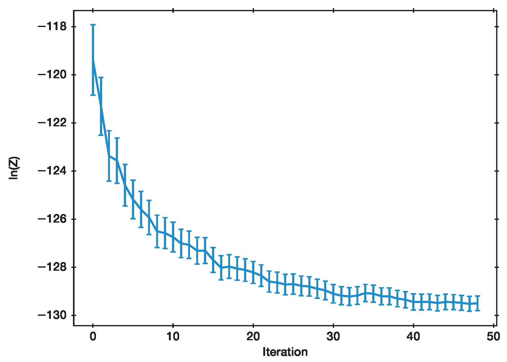
We test the algorithm on the Rosenbrock function over a flat prior from −10 to +10 in $d=20$ dimensions. The likelihood is:

$$ln\mathcal{L}\left(\theta \right)=-2\times \sum _i\left(100\times \left({\theta }_{i+1}-{\theta }_i^2\right){}^2+{\left(1-{\theta }_i\right)}^2\right)$$

With $K_0=20$, and $K_{\mathrm{inc}}=20$, and $M=20$, we observe that $ln\left(Z\right)$ evolves as shown in Figure 1. From an initial high value, the estimate declines approximately proportional to $1/(M\times K)$ towards the (presumably true) value if nested sampling was run with $K=\infty$.

4. Discussion

We have presented an iterative form of applying nested sampling. It can be understood as a kind of dynamic nested sampling. The proposed algorithm has several amicable properties:

• the number of live points and the number of steps do not have to be chosen carefully,
• an initial quick look result is available,
• the evidence estimate improves as more compute is added,
• in multi-modal settings, additional peaks are discovered as more compute is added,
• the convergence can be observed and tested with conventional methods based on MCMC,
• the posterior sample size increases proportionally to the compute,
• it is easy to implement.

The convergence as more compute is added, the revisiting and further exploration of missed peaks, and the possibility to use conventional MCMC convergence diagnostics, are properties shared with diffusive nested sampling [14]. That algorithm is based on likelihood levels. Instead of monotonically switching to higher likelihoods, the sampler can randomly go up or down in levels, and add more samples (live points) there. Unlike diffusive nested sampling, snowballing nested sampling provides an uncertainty estimate on the evidence Z.

Finally, we make some remarks on adaptive MCMC algorithms. Salomone et al. [6] pointed out that on-the-fly adaptation of MCMC algorithms is problematic, and a warm-up nested sampling run should be performed, the adapted proposal kernel (parameters) at each iteration stored, and applied without adaptation in a second, fresh nested sampling run. If the MCMC transition kernel is created based on estimating a sample covariance matrix of the live point population, this estimate stabilizes as K increases. Newly added $K_{\mathrm{inc}}$ live points only mildly alter the estimate as $K\to \infty$. Another popular adaptation is to alter the proposal scale in Metropolis random walks to target a certain acceptance rate. If the proposal scale is chosen based on the acceptance rate of the previous K points and their proposal scale, through a weighted mean targeting an acceptance rate of 23.4 percent, then we have a situation of a vanishing adaptation see [15] with convergence to the true posterior. Furthermore, as the sampling is more faithful, the live points are also more faithfully distributed, which in turn improves the sampling, leading to a positive feedback effect. This accelerates the convergence further.

References

- Skilling, J. Nested sampling. AIP Conf. Proc. 2004, 735, 395. [Google Scholar] [CrossRef]
- Ashton, G.; Bernstein, N.; Buchner, J.; Chen, X.; Csányi, G.; Fowlie, A.; Feroz, F.; Griffiths, M.; Handley, W.; Habeck, M.; et al. Nested sampling for physical scientists. arXiv 2022, arXiv:2205.15570. [Google Scholar] [CrossRef]
- Buchner, J. Nested Sampling Methods. arXiv 2021, arXiv:2101.09675. [Google Scholar] [CrossRef]
- Handley, W.J.; Hobson, M.P.; Lasenby, A.N. POLYCHORD: Nested sampling for cosmology. MNRAS 2015, 450, L61–L65. [Google Scholar] [CrossRef]
- Buchner, J. Comparison of Step Samplers for Nested Sampling. Phys. Sci. Forum 2022, 5, 46. [Google Scholar] [CrossRef]
- Salomone, R.; South, L.F.; Drovandi, C.C.; Kroese, D.P. Unbiased and Consistent Nested Sampling via Sequential Monte Carlo. arXiv 2018, arXiv:1805.03924. [Google Scholar]
- Higson, E.; Handley, W.; Hobson, M.; Lasenby, A. NESTCHECK: Diagnostic tests for nested sampling calculations. MNRAS 2019, 483, 2044–2056. [Google Scholar] [CrossRef]
- Higson, E.; Handley, W.; Hobson, M.; Lasenby, A. Dynamic nested sampling: An improved algorithm for parameter estimation and evidence calculation. arXiv 2017, arXiv:1704.03459. [Google Scholar] [CrossRef]
- Chopin, N.; Robert, C.P. Properties of nested sampling. Biometrika 2010, 97, 741–755. [Google Scholar] [CrossRef]
- Chopin, N.; Robert, C. Contemplating Evidence: Properties, Extensions of, and Alternatives to Nested Sampling; Technical report, Technical Report 2007-46; CEREMADE, Université Paris Dauphine: Paris, France, 2007. [Google Scholar]
- Skilling, J. Nested sampling’s convergence. AIP Conf. Proc. 2009, 1193, 277–291. [Google Scholar] [CrossRef]
- Skilling, J. Nested sampling for general Bayesian computation. Bayesian Anal. 2006, 1, 833–859. [Google Scholar] [CrossRef]
- Speagle, J.S. DYNESTY: A dynamic nested sampling package for estimating Bayesian posteriors and evidences. MNRAS 2020, 493, 3132–3158. [Google Scholar] [CrossRef]
- Brewer, B.J.; Pártay, L.B.; Csányi, G. Diffusive nested sampling. Stat. Comput. 2011, 21, 649–656. [Google Scholar] [CrossRef]
- Andrieu, C.; Thoms, J. A tutorial on adaptive MCMC. Stat. Comput. 2008, 18, 343–373. [Google Scholar] [CrossRef]
Figure 1.
Estimate of for each algorithm iteration.
Disclaimer/Publisher’s Note: The statements, opinions and data contained in all publications are solely those of the individual author(s) and contributor(s) and not of MDPI and/or the editor(s). MDPI and/or the editor(s) disclaim responsibility for any injury to people or property resulting from any ideas, methods, instructions or products referred to in the content. |
© 2023 by the author. Licensee MDPI, Basel, Switzerland. This article is an open access article distributed under the terms and conditions of the Creative Commons Attribution (CC BY) license (https://creativecommons.org/licenses/by/4.0/).
Share and Cite
MDPI and ACS Style
Buchner, J. Snowballing Nested Sampling. Phys. Sci. Forum 2023, 9, 17. https://doi.org/10.3390/psf2023009017
AMA Style
Buchner J. Snowballing Nested Sampling. Physical Sciences Forum. 2023; 9(1):17. https://doi.org/10.3390/psf2023009017
Chicago/Turabian StyleBuchner, Johannes. 2023. "Snowballing Nested Sampling" Physical Sciences Forum 9, no. 1: 17. https://doi.org/10.3390/psf2023009017