The GRB Afterglows Flowchart ^†

Abstract

In this paper, we present a flowchart of the Gamma Ray Burst (GRB) afterglows, aiming to create a numerical FORTRAN code. Considering several proposed models, the hydrodynamic evolution describing the external shock of the jet with the environment surrounding the GRB source or the Interstellar medium is discussed. A comparison of the results and data, considering the synchrotron emission as a basic mechanism for the radiation part, was also carried out.

1. Introduction

“Gamma-Ray Bursts observations of a cosmic origin” is the title of the first article on this subject, published in 1973 [1], in which it was announced that this is the brightest event in the universe after the Bing Bang. Since then, many satellite missions and terrestrial projects have been carried out to solve this enigma. One of these satellites, called Beppo-SAX, definitively confirmed the cosmological origin of these bursts by detecting the first remnant emission (afterglow) of the GRB970228 with a Redshift = 0.835 [2], defined as the external shock of the jet with the environmental medium of the source of the gamma rays burst [3]. Most theorists focused their studies on the fireball model [4,5,6], which can describe the external shock. Accordingly, three hydrodynamic models were proposed in the literature to describe the evolution of the Lorentz factor: those of Chiang Dermer (1999) [7], Huang et al. (1999) [8] and Feng et al. (2002) [9]. A flowchart of these models will be presented in the following.

2. Hydrodynamic Evolution

2.1. Hydrodynamic Models

The bulk kinetic energy of the GRB fireball is expressed by [10]:

$$E_k=(\Gamma -1)(M_0+m)c^2+\Gamma U$$

(1)

where $\Gamma$ is the bulk Lorentz factor of the deceleration, m the mass of the surrounding medium that is swept up by the fireball. The radiated differential energy is given by [11]:

$$d{E}_{rad}=\epsilon \Gamma (\Gamma -1)dm{c}^2$$

(2)

and

$$\epsilon ={\epsilon }_e\frac{{t^{{}^{\prime }}}_{syn}^{-1}}{{t^{{}^{\prime }}}_{syn}^{-1}+{t^{{}^{\prime }}}_{ex}^{-1}}$$

(3)

where $\epsilon$ is the fraction of internal energy radiated by the fireball [12,13], $t_{syn}$, $t_{ex}$ are the synchrotron cooling and expansion times in the co-moving frame, respectively, and U is the internal energy, which has has many proposed definitions, as shown in

Table 1. Different internal energy for each model and its Lorentz factor evolution.

Models	Internal Energy		Lorentz Factor Evolution
Chaing [7]	$U=\int (\Gamma -1)dm$	$dU=(\Gamma -1)dm$	$\frac{d\Gamma }{dm}=-\frac{{\Gamma }^2-1}{M}$
Huang [8]	$U=(\Gamma -1)m{c}^2$	$dU=(\Gamma -1)dm{c}^2+m{c}^{2}d\Gamma$	$\frac{d\Gamma }{dm}=-\frac{{\Gamma }^2-1}{M_0+\epsilon m+2(1-\epsilon )\Gamma m}$
Feng [9]	$U=\int (1-\epsilon )d{U}_{ex}$	$dU=(1-\epsilon )d{U}_{ex}\backslash \backslash d{U}_{ex}=(\Gamma -1)dm{c}^2+m{c}^{2}d\Gamma$	$\frac{d\Gamma }{dm}=-\frac{{\Gamma }^2-1}{M_0+m+U/c^2+(1-\epsilon )\Gamma m}$

. Finally, the global conservation of energy is $d{E}_k=-d{E}_{rad}$, where the evolution of the Lorentz factor $\Gamma$ can describe the hydrodynamic evolution of the GRBs afterglows, as shown in Table 1.

2.2. The Flowchart of the Hydrodynamic Evolution

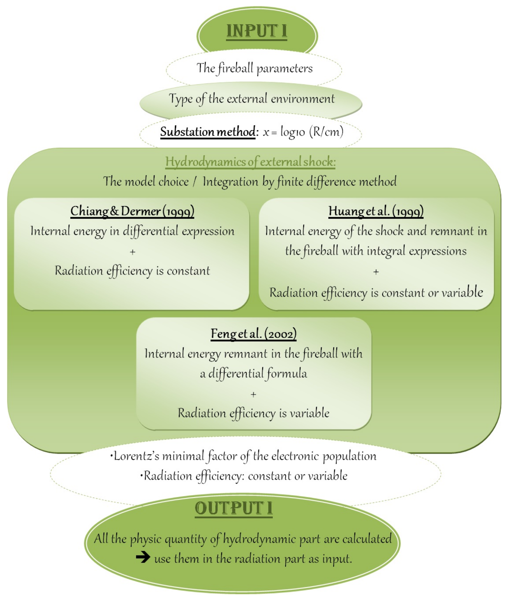
The basic aim of this work is to draw a flowchart of the hydrodynamic evolution for the GRB afterglows, then choose the most compatible model using the observational data (see Section 3.2). All steps for the first part are shown in Figure 1:

• Start with the initial parameters for all necessary physical quantities, such as those of the fireball and the external environment.
• Use the substitution $x={log}_{10}$ (R/cm) (logarithmic scale), which is suitable for large scales, dealing with large distances and long periods of time, such as the distance traveled.
• Specify the state of the fireball, such as whether it is radiated, constant or variable (depending on the effectiveness of the radiation). We will also choose a model with a minimum Lorentz factor.
• Choose the hydrodynamic model, then use the finite differences method as a numerical tool to obtain approximate solutions of the Lorentz factor differential equations as a function of the mass m of the surrounding medium that is swept up by the fireball. This method appears to be the simplest one. Furthermore, using this method in our code provides results that converge to the Sedov solution [14], and to the analytical solutions in case of an expanded and constant radiation.

3. Radiation Parte

3.1. Synchrotron Radiation and Self-Absorption

The synchrotron radiation power (OTS) at frequency ${\nu }^{\prime }$ from all the accelerated electrons in the commoving frame is given by [15]:

$$P_{{\nu }^{\prime }}=\frac{2\sqrt{3}{e}^2{\nu }_L}{c}{\int }_{{\Gamma }_{min}}^{{\Gamma }_{max}}{N}_e^{\prime }\left({\Gamma }_e\right)F\left(\frac{{\nu }^{\prime }}{{\nu }_c^{\prime }}\right)d{\Gamma }_e$$

(4)

where $F\left(x\right)$ is the symchrotron function [16], ${\nu }_L$ is the Larmor frequency and $N_e^{\prime }$ represents the electrons accelerated by the shock in the absence of radiation losses, written as a bower low distribution [13]:

$$N_e^{\prime }\left({\Gamma }_e\right)=\frac{d{N}_e^{\prime }}{d{\Gamma }_e}=C^{te}{\Gamma }_e^{-P},{\Gamma }_{min}\le {\Gamma }_e\le {\Gamma }_{max}$$

(5)

where ${\Gamma }_{max}$ (resp. ${\Gamma }_{min}$) is defined in [17,18] (resp. [19]).

Due to the cosmological nature of the GRBs, we must use the relativistic transformations: [15,20]:

$$\nu =\frac{(1+\beta )\Gamma }{1+z}{\nu }^{\prime }$$

(6)

$$d\Omega =\frac{1}{{(1+\beta )}^2{\Gamma }^2}d{\Omega }^{\prime }$$

(7)

$$t_{obs}=(1+z)t$$

(8)

to obtain the general expression of the instantaneous intensity in the Jansky of synchrotron emission as a function of the luminosity distance $D_L\left(z\right)$, where z is the redshift:

$${\left(F_{\nu }\right)}_{OTS}=\frac{1}{4\pi D_L{\left(z\right)}^2}4\pi {\left(\frac{d{P}_{\nu }}{d\Gamma }\right)}_{OTS}$$

(9)

The synchrotron self-absorption (SSA) at low frequencies plays an important role; when ${\alpha }_{{\nu }^{\prime }}$, the optical depth is [21]:

$${\alpha }_{{\nu }^{\prime }}=\frac{(p+1)}{8\Pi m_e{\nu }^{\prime }}{\int }_{{\Gamma }_{min}}^{{\Gamma }_{max}}{P}_e^{\prime }\left({\Gamma }_{{\nu }^{\prime },e}\right)\frac{N_e^{\prime }\left({\Gamma }_e\right)}{{\Gamma }_e}d{\Gamma }_e$$

(10)

so the instantaneous intensity for the SSA will be [22]:

$${\left(\frac{d{P}_{\nu }}{d\Gamma }\right)}_{SSA}={\left(\frac{d{P}_{\nu }}{d\Gamma }\right)}_{OTS}\frac{1}{{\alpha }_{{\nu }^{\prime }}{\Delta }^{\prime }}(1-e^{{\alpha }_{{\nu }^{\prime }{\Delta }^{\prime }}})$$

(11)

3.2. The Flowchart of the Radiation Emission

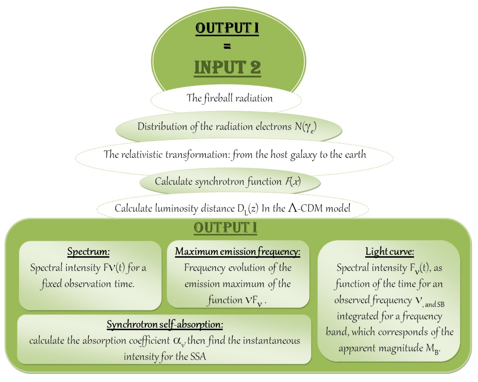
In the second part (Figure 2), we produce the light curves represented by the intensity as a function of time Equation (9). Similarly for the afterglow spectra, the same quantity is used as a function of the frequency.

Finally, the numerical curve presenting the frequency of the maximum emission is presented in terms of $\nu F\left(\nu \right)$.

• To observe the nature of the energy emitted by the afterglows as a function of time with the light curves, we introduce the frequency in the observations, then create a DO loop for various time values to calculate the spectral intensity $F_{\nu }\left(t\right)$. In this loop, we call the subroutines of the relativistic transformation for each distance R.
• For the spectra, the opposite is carried out; that is, we set the time then open a DO loop to evolve the frequency, and call the subroutine of the relativistic transformation at every distance R.
• For the third calculations, we make changes to the time and frequency with two DO loops and use the condition IF to save the frequency that gives the maximum of $\nu F\left(\nu \right)$.

To recognize this part, we use the $F\left(x\right)$ synchrotron function to determine the spectral power, by calculate the distribution of the radiating electrions, and consider the numbers of the electrons that radiate or do not radiate (adiabatic electrons, for which the characteristic time of emission is very small compared to the time scales). We identify all the relativistic transformations representing the physical quantities in the host galaxy $({\nu }^{\prime },d\Omega )$ due to the cosmological distance, which is used as the luminosity distance $D_L\left(z\right)$. Finally, we calculate the absorption coefficient ${\alpha }_{{\nu }^{\prime }}$ Equation (10) to obtain the instantaneous intensity for the SSA Equation (11) and present our results.

4. Numerical Results and Discussion

We used a fireball with an initial mass outflow, $M_0=2\times {10}^{-6}{M}_{\odot }$, Lorentz factor ${\Gamma }_0=65$ and a half-opening angle of the jet ${\theta }_{jet}={10}^{\circ }$, a deceleration within the ISM with a constant density $n=1$ cm${}^3$ and $k=0$ (n, k are parameters depending on the medium), $z=3.645$, lateral expansion $g=0$, numerical and spectral parameters $a=4$ and $p=2.3$, respectively. We also used ${\epsilon }_e=0.1$, ${\epsilon }_B=0.9$ as the electronic and magnetic efficiencies, with ${\epsilon }_e+{\epsilon }_B=1$. The main goal of this code is to study and understand this phenomenon. In fact, using this flowchart, we highlighted the most important results:

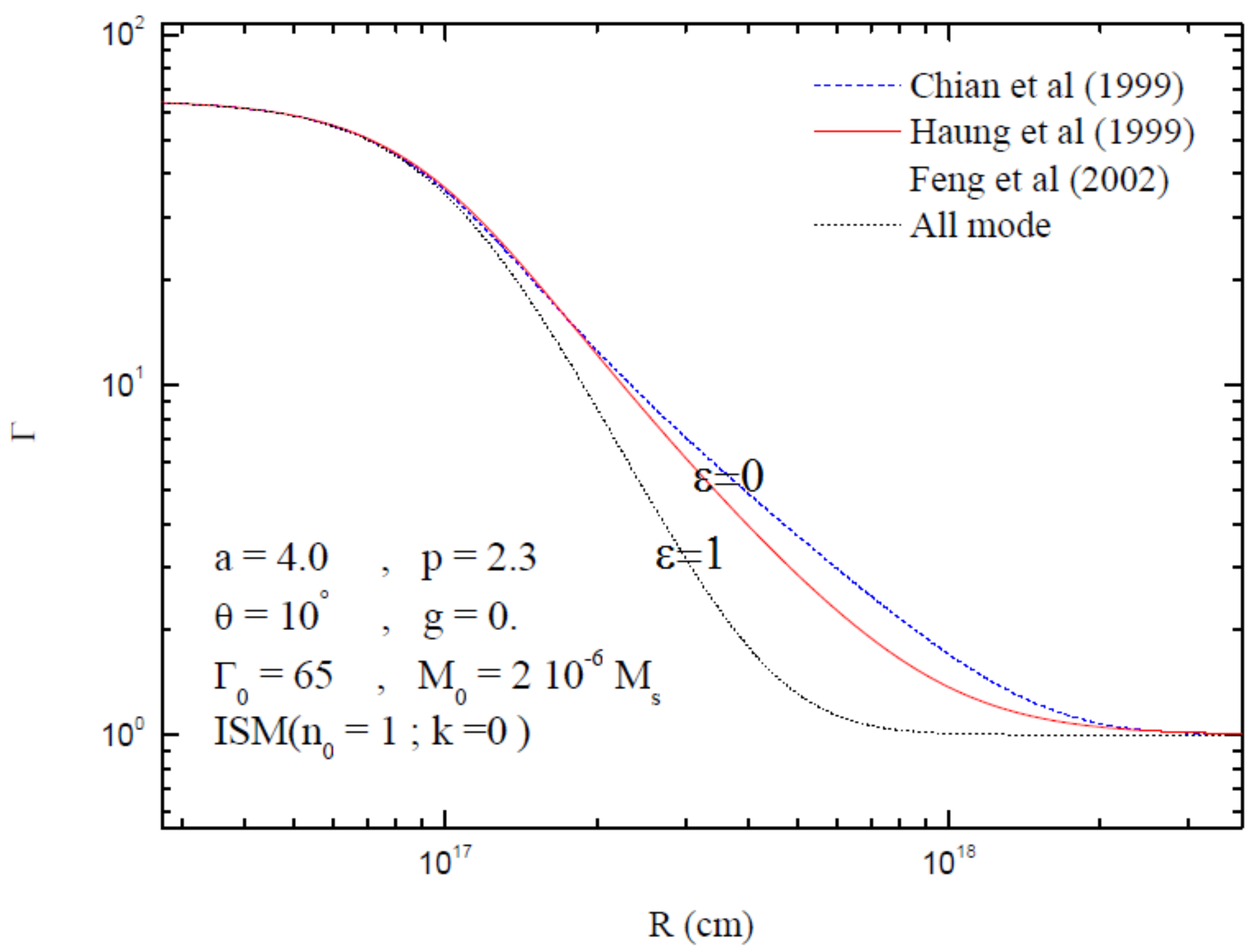
• Figure 3 shows that, in the adiabatic expansion case, the deceleration of the Lorentz factor is slower compared to that of a radiative regime that generates a faster deceleration due to radiation. Moreover, we can observe three sections of the deceleration, corresponding to:

  1.

  The ultra-relativistic phase.

  2.

  The relativistic phase.

  3.

  The non-relativistic phase.

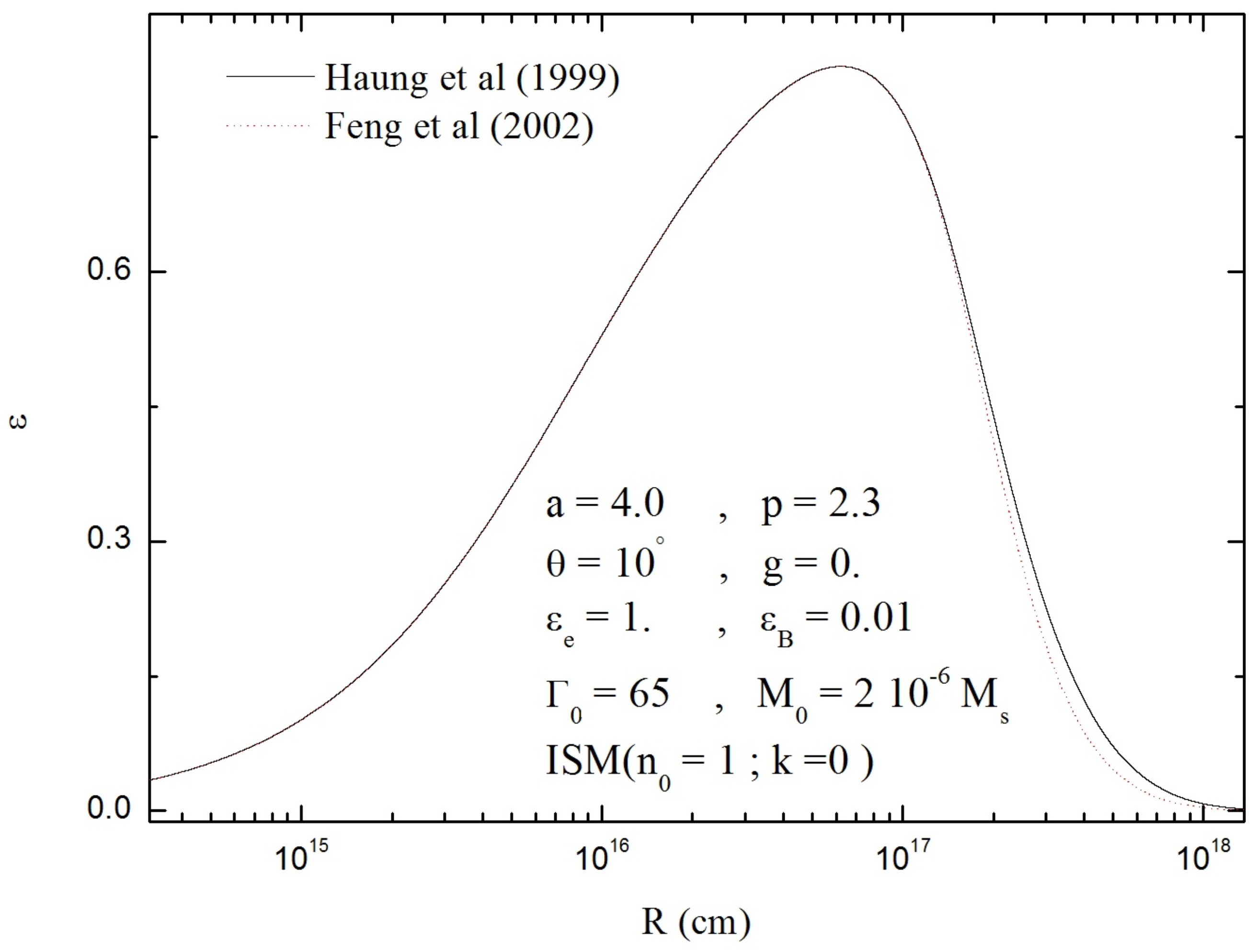
• Figure 4 displays the evolution of the radiative efficiency of the fireball as a function of the distance R, showing that the radiation in Haung’s models is more effective than that of Feng.
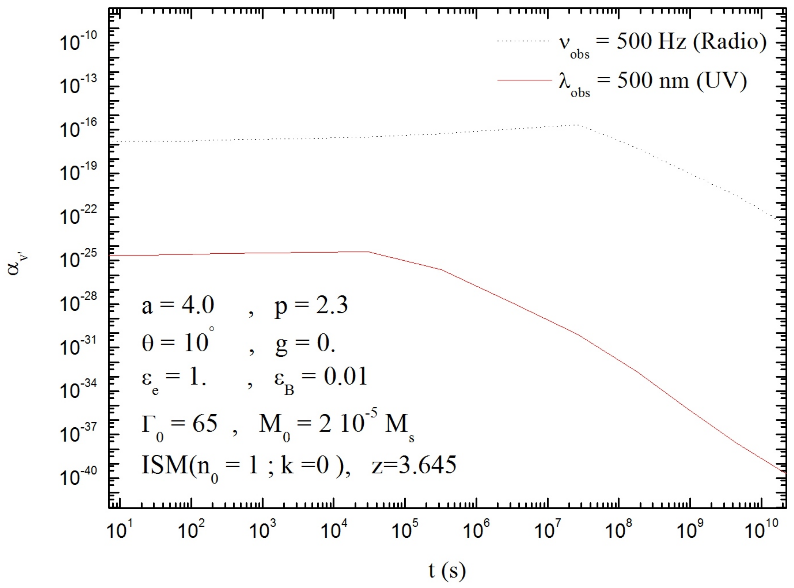
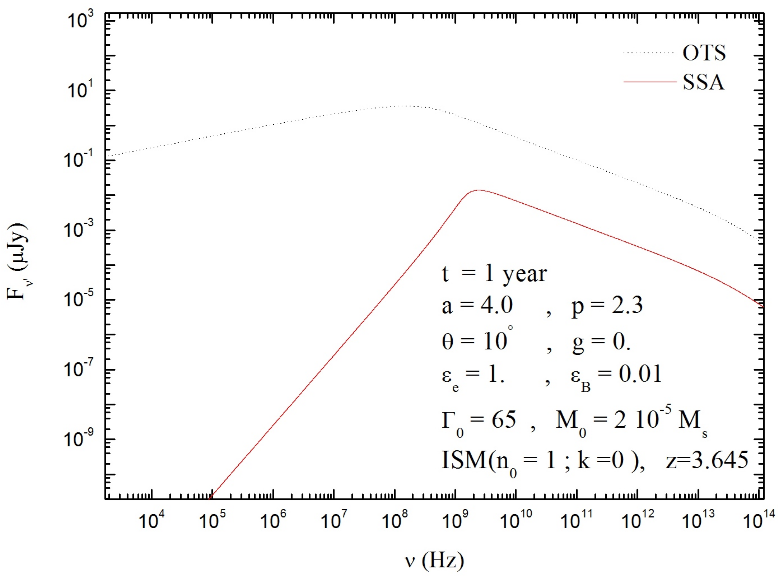
• Figure 5 shows the ratio between the absorption coefficient ${\alpha }_{{\nu }^{\prime }}$ for a radio frequency ${\nu }_{obs}=3·{10}^8 \mathrm{H}\mathrm{z}$ and an UV one ${\lambda }_{obs}^{-1}=500 \mathrm{c}{\mathrm{m}}^{-1}$. Note that this is more important at low frequencies. This result is confirmed in Figure 6, where the spectra of GRB afterglow consist of an increased absorption at low frequencies compared to higher frequencies.
• Figure 7 shows that the majority of the radiation during the GRB-afterglow emissions starts by the hard gamma to the radio bands. Therefore, the detection of the prompt emission of GRBs overlaps with the early afterglows
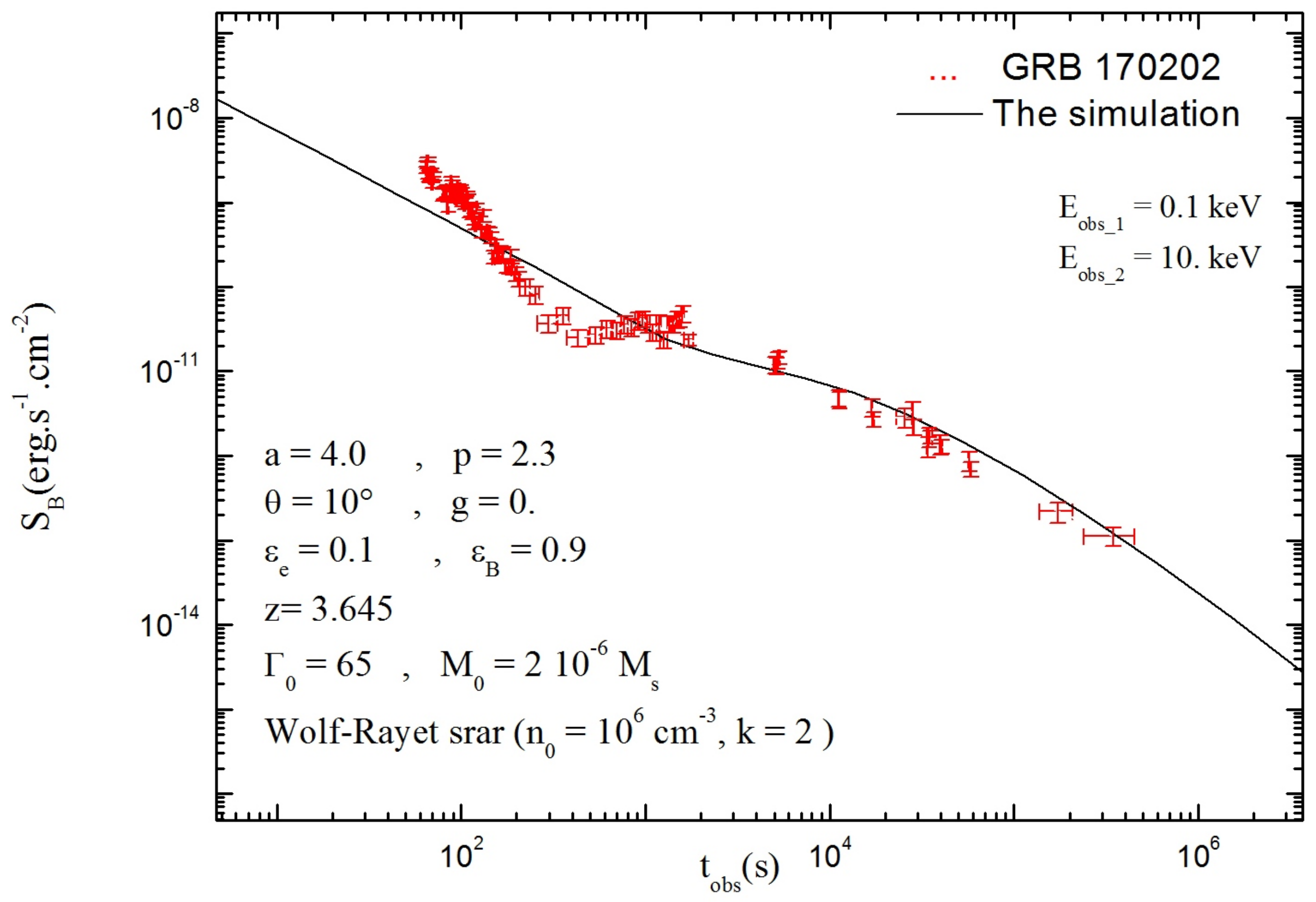
• Figure 8 shows a good concordance between the GRB170202 data supporting the proposed model.

5. Conclusions

In the presented work, we studied the evolving hydrodynamics of the afterglow and its emission. We show that the Feng’s model is the most interesting [23,24]. From the perspective of efficiency, the changes made later in the evolution of the fireball make it more realistic to describe the internal energy. It is worth mentioning that the Feng models are consistent with the Sedov solution, both the non-relativistic phase and adiabatic regime. We then studied the basic radiation of the GRB afterglow using the synchrotron emissions, which are not negligible. The self synchrotron absorption is an effect that plays an important role in the low-frequency range, providing a fairly good approximation of the real data, as in our case, where the profile of the GRB 170202 afterglow was detected by Swift/XRT.

References

- Klebesadel, R.W.; Strong, I.B.; Olson, R.A. Observation of Gamma-Ray Bursts of Cosmic Origin. Astrophys. J. 1973, 182, L85–L88. [Google Scholar] [CrossRef]
- Costa, E.; Frontera, F.; Heise, J.; Feroci, M.; in ’t Zand, J.; Fiore, F.; Cinti, M.N.; Fiume, D.D.; Nicastro, L.; Orlandini, M.; et al. Discovery of an X-ray afterglow associated with the γ-ray burst of 28 February 1997. Nature 1997, 387, 783–785. [Google Scholar] [CrossRef]
- Shaviv, N.J.; Dar, A. Fireballs in dense stllar regions as an explanation of gamma-ray bursts. Mon. Not. R. Astron. Soc. 1995, 277, 287–296. [Google Scholar]
- Sari, R.; Piran, T. Variability in gamma-ray bursts: A clue. Astrophys. J. 1997, 485, 270–273. [Google Scholar] [CrossRef]
- Dermer, C.D.; Mitman, K.E. Short-timescale variability in the external shock model of gamma-ray bursts. Astrophys. J. 1999, 513, L5–L8. [Google Scholar] [CrossRef]
- Zouaoui, E.; Mebarki, N.; Benslama, A. A dynamical evolution of GRB-afterglows in a new generic model. Mod. Phys. Lett. A 2021, 36, 2150268. [Google Scholar] [CrossRef]
- Chiang, J.; Dermer, C.D. Synchrotron and synchrotron self-compton emission and the blast-wave model of gamma-ray bursts. Astrophys. J. 1999, 512, 699–710. [Google Scholar] [CrossRef]
- Huang, Y.F.; Dai, Z.G.; Lu, T. A generic dynamical model of gamma-ray burst remnants. Mon. Not. R. Astron. Soc. 1999, 309, 513–516. [Google Scholar] [CrossRef]
- Feng, J.B.; Huang, Y.F.; Dai, Z.G.; Lu, T. Dynamical evolution of gamma-ray burst remnants with evolving radiative efficiency. Chin. J. Astron. Astrophys. 2002, 2, 525–532. [Google Scholar] [CrossRef]
- Panaitescu, A.; Mészáros, P.; Rees, M.J. Multiwavelength afterglows in gamma-ray bursts: Refreshed shock and jet effects. Astrophys. J. 1998, 503, 314–315. [Google Scholar] [CrossRef]
- Blandford, R.D.; McKee, C.F. Fluid dynamics of relativistic blast waves. Phys. Fluids 1976, 19, 1130–1138. [Google Scholar] [CrossRef]
- Dai, Z.G.; Lu, T. Gamma-ray burst afterglows: Effects of radiative corrections and non-uniformity of the surrounding medium. Mon. Not. R. Astron. Soc. 1998, 298, 87–92. [Google Scholar] [CrossRef]
- Dai, Z.G.; Huang, Y.F.; Lu, T. Gamma-ray burst afterglows from realistic fireballs. Astrophys. J. 1999, 520, 634–640. [Google Scholar] [CrossRef]
- Sedov, L. Similarity and Dimensional Methods in Mechanics; Ch. IV; Academic: New York, NY, USA, 1969. [Google Scholar]
- Rybicki, G.B.; Lightman, A.P. Radiative Processes in Astrophysics; Wiley and Sons: New York, NY, USA, 1979. [Google Scholar]
- Abramowiotz, M.; Stegum, I.A. Handbook of Mathematical Function; Dover: New York, NY, USA, 1965. [Google Scholar]
- De jager, O.C.; Harding, A.K. The expected high-energy to ultra-high-energy gamma-ray spectrum of the Crab Nebula. Astrophys. J. 1992, 4396, 161–172. [Google Scholar] [CrossRef]
- De Jager, O.C.; Harding, A.K.; Michelson, P.F.; Nel, H.I.; Nolan, P.L.; Sreekumar, P.; Thompson, D.J. Gamma-Ray Observations of the Crab Nebula: A Study of the Synchro-Compton Spectrum. Astrophys. J. 1996, 457, 253–266. [Google Scholar] [CrossRef]
- Sari, R.; Piran, T.; Narayan, R. Spectra and light curves of gamma-ray burst afterglows. Astrophys. J. Lett. 1998, 497, L17–L20. [Google Scholar] [CrossRef]
- Lind, K.R.; Blandford, R.D. Semidynamical models of radio jets-Relativistic beaming and source counts. Astrophys. J. 1985, 295, 358–367. [Google Scholar] [CrossRef]
- Jonathan, G.; Tsvi, P.; Reém, S. Synchrotron self-absorption in gamma-ray burst afterglow. Astrophys. J. 1999, 527, 236–246. [Google Scholar]
- Zouaoui, E.; Mebarki, N. Synchrotron Emission and Self-Absorption in GRB Afterglows. J. Phys. Conf. Ser. 2019, 1269, 012010. [Google Scholar] [CrossRef]
- Zouaoui, E.; Fouka, M.; Ouichaoui, S. Hydrodynamical Evolution of GRBs Afterglows: Realistic model with evolving radiative efficiency. Aip Conf. Proc. 2012, 1444, 359–362. [Google Scholar]
- Zouaoui, E.; Fouka, M.; Ouichaoui, S. L’evolution hydrodynamique des afterglows pour le modele de feng. Sci. Technol. A 2015, 41, 71–74. [Google Scholar]
Figure 1.
The flowchart of the hydrodynamic evolution of GRBs afterglows for Chiang Dermer (1999) [7], Huang et al. (1999) [8] and Feng et al. (2002) [9].
Figure 2.
The flowchart of the radiation of GRBs’ afterglows.
Figure 3.
Evolution of the Lorentz factor as a function of the distance R (in logarithmic scale), for Chiang Dermer (1999) [7], Huang et al. (1999) [8] and Feng et al. (2002) [9], for radiative and adiabatic cases.
Figure 4.
Evolution of the radiative efficiency of the fireball as a function of the distance R (in logarithmic scale), for Chiang Dermer (1999) [7], Huang et al. (1999) [8] and Feng et al. (2002) [9].
Figure 5.
Evolution of absorption coeffcient for radio frequency and UV frequency (for Feng model).
Figure 6.
Spectra of GRB afterglow in the two cases of OTS and SSA emissions (for Feng model).
Figure 7.
Frequency corresponding to the maximum emission in terms of as a function of the distance R (for Feng model).
Figure 8.
Comparison of calculated afterglow light curves (our code) to the observed data using the XRT / Swift satellite, considering of the integrated fluence, (in erg.s.cm units) in the X-ray band (E = 0.2–10 keV).
Disclaimer/Publisher’s Note: The statements, opinions and data contained in all publications are solely those of the individual author(s) and contributor(s) and not of MDPI and/or the editor(s). MDPI and/or the editor(s) disclaim responsibility for any injury to people or property resulting from any ideas, methods, instructions or products referred to in the content. |
© 2023 by the authors. Licensee MDPI, Basel, Switzerland. This article is an open access article distributed under the terms and conditions of the Creative Commons Attribution (CC BY) license (https://creativecommons.org/licenses/by/4.0/).
Share and Cite
MDPI and ACS Style
Zouaoui, E.; Mebarki, N. The GRB Afterglows Flowchart. Phys. Sci. Forum 2023, 7, 51. https://doi.org/10.3390/ECU2023-14045
AMA Style
Zouaoui E, Mebarki N. The GRB Afterglows Flowchart. Physical Sciences Forum. 2023; 7(1):51. https://doi.org/10.3390/ECU2023-14045
Chicago/Turabian StyleZouaoui, Esma, and Noureddine Mebarki. 2023. "The GRB Afterglows Flowchart" Physical Sciences Forum 7, no. 1: 51. https://doi.org/10.3390/ECU2023-14045