
Is Quantum Tomography a Difficult Problem for Machine Learning? †

Inria Saclay Ile-de-France, 91120 Palaiseau, France
†
Presented at the 41st International Workshop on Bayesian Inference and Maximum Entropy Methods in Science and Engineering, Paris, France, 18–22 July 2022.
Phys. Sci. Forum 2022, 5(1), 47; https://doi.org/10.3390/psf2022005047
Published: 7 February 2023
(This article belongs to the Proceedings of The 41st International Workshop on Bayesian Inference and Maximum Entropy Methods in Science and Engineering)
Abstract
:One of the key issues in machine learning is the characterization of the learnability of a problem. Regret is a way to quantify learnability. Quantum tomography is a special case of machine learning where the training set is a set of quantum measurements and the ground truth is the result of these measurements, but nothing is known about the hidden quantum system. We will show that in some case quantum tomography is a hard problem to learn. We consider a problem related to optical fiber communication where information is encoded in photon polarizations. We will show that the learning regret cannot decay faster than where T is the size of the training dataset and that incremental gradient descent may converge worse.
1. Introduction: Supervised Learning in General
With the invention of deep neural learning, the general public thinks there is a glimpse of a universal machine learning technology capable of solving arbitrary problems without any specific preparation on training data and learning strategy. Everything “is” be solvable as long as there are enough layers, enough processing power and enough training data. We arrived at the point that many people (among them the late Stephen Hawking) start thinking that machines may supersede human intelligence thanks to the greater performance of silicon neurons over biological neurons, and may be capable of cracking the last enigmas around the physical nature of the universe.
However, we should not forget that actual Artificial Intelligence (AI) has many limitations. However, due to the youth of technology, many of the present limits might be of teething nature. To learn a language the present algorithms need to be trained over millions of texts which is equivalent to a training period of 80 years if it were done at the learning pace of a child! Presently, deep neural training is very demanding in processing and it is the third major source of energy consumption among information technologies after Bitcoin and data centers. Deep learning is not yet such a good self-organizing learning process as some researchers would have thought [1]. There is also the obstacle of data sparsity to learning (the machine only recognizes the data on which it has been trained over and over as if a reader could only understand the texts on which (s)he has been trained).
To make it short the main limitations of machine learning technologies are: (i) the data sparsity; (ii) the absence of a computable solution to learn (e.g., the program halting problem); (iii) the presence of hard-to-learn algorithms in the solution. My present paper will address the third limitation.
A supervised learning problem can be viewed as a set of training data and ground truths. The machine acts as an automaton whose aim is to predict the ground truth from data. The loss measures the difference between the prediction and the ground truth and can be established under an arbitrary metric. The general objective of supervised machine learning is to minimize the average loss, but since the ground truth might contain some inherent stochastic variations (e.g., when predicting the result of a quantum measurement) it may be impossible to make the loss as small as we would like. Given an automaton architecture, there exists a setting that gives the optimal average loss. However, the optimal setting might be difficult to reach. However, there is still the question of the size of the training set needed to converge to the optimal settings.
All problems are not equal in front of learnability [2]. Some seem to be a perfect match with AI, some others are more difficult to adapt. In [3], the author shows that the random parity functions are just unlearnable. In fact, in a broader perspective, the “learnability” may not be a learnable problem [4].
The first contribution of this paper is a new definition of learning regret with respect to a given single problem submitted to a given learning strategy. Most regret expressions are infimum of regret over a large class (if not universal) of problems [5] and therefore lose the specificity of individual problems.
The second contribution is the application of this new regret definition to a quantum tomography problem. The specificity of the problem is that the hidden source probability distribution is indeed contained in the learning distribution class. The surprising result is that the regret is at least in the square root of the number of runs, hinting at a poor convergence rate of the learned distribution toward the hidden distribution. We conclude with numerical experiments with gradient descents.
2. Expressing the Convergence Regret
Let T be an integer and let be a sequence of features which are vectors of a certain dimension which define the problem (the notation with T is not for “transpose”, which should be noted , but for a sequence with T atoms). Each feature generates a discrete random label y. Let denote (S for “source”) the probability to have label y given the feature . If is the sequence of random labels given the sequence of feature : . The sequence of features and labels defines the problem for supervised learning.
The learning process will give as output an index which will be taken from a set of , such that each define a distribution (L for “learning”) over the label sequence given the feature sequence. In absence of side information the learning process leads to . Our aim is find how close is to when varies.
The distance between the two distributions can be expressed by the Kullback–Leibler divergence [6]
However, it should be stressed that the quantity does not necessarily define a probability distribution since may vary when varies, making equal to 1 unlikely. Thus, is not a distance, because it can be non-positive. One way to get through is to introduce with which makes a probability distribution. Thus, we will use which satisfies:
and is now a well-defined semi distance which we will define as the learning regret [5].
3. The Quantum Learning on Polarized Photons
We now include pure physical measurements in the learning process. There are several applications that involve physic, ref. [7] describes a process of deep learning over the physical layer of a wireless network. The issue with quantum physical effects is the fact that they are not reproducible and not deterministic. We consider a problem related to optical fiber communication where information is encoded in photon polarizations. The photon polarization is given by a quantum wave function of dimension 2. In the binary case, the bit 0 is given by polarisation angles and the bit 1 is given by angle . The quantity is supposed to be unknown by the receiver and its estimate is obtained after a training sequence via machine learning.
For this purpose, the sender sends a sequence of T equally polarized photons, along angle , the receiver measures these photons over a collection of T measurement angles , called the featured angles. They are pure scalar and are not vector (), therefore we will not depict them in bold font as in the previous section which is therefore of dimension 1. The labels, or ground truths, are the sequence of binary measurement obtained, , there are possible label sequences.
This problem is the most simplified version of tomography on quantum telecommunication since it relies on a single parameter. More realistic and more complicated situations will occur when noisy circular polarization is introduced within a more complex combination of polarizations within groups of photons. This will considerably increase the dimension of the feature vectors and certainly will make our results on the training process more critical. However, in the situation analyzed in our paper, we show that this simple system is difficult to learn.
If we assume that the experiment results are delivered in batches to the training process, that is the estimate does not vary for , the learning class of probability distribution is a function of with . The source distribution is indeed , thus the source distribution belongs to the class of learning distribution. For a given pair of sequence , let be the value of which maximizes . Since we will never touch the sequence which are the foundation of the experiments, we will sometimes drop the parameter and denote . The quantity which maximizes will satisfy . We have
We notice that for all is always strictly positive (but and are not continuous so ℓ is not convex). We now turn to displaying and proving our main results (two theorems), whose proof would need the following two next lemmas.
Lemma 1.
We have the expression
Proof.
Let which is homomorphic and is locally invertible (since is never zero). Let we denote the function . We have . For , let be the Fourier transform of function . Formally we have
and inversely
Thus
□
In fact, the function may have several extrema as we will see in the next section, thus may have several roots, thus is polymorphic. In order to avoid the secondary roots which contribute to the non-optimal extrema, we will concentrate on the main root in the vicinity of .
Let and be two sequence of real numbers. We denote .
Lemma 2.
For any we have the identity
For , we have
Proof.
This is just the consequence of the finite sums via algebraic manipulations. □
Theorem 1.
Under mild conditions, we have the estimate
Proof.
Let . Applying both lemma with and , thus we get
with
We notice that with
We notice that and when . The expression is obtained via saddle point method approximation, under the mild conditions being that it can be applied as in the maximum likelihood problem [8] (the error term would be the smallest possible)
with , and Since , the factor behaves like a gaussian function centered on with standard deviation of order . Thus, via saddle point approximation again, it comes:
with with is clearly .
Furthermore, , thus we have
□
Theorem 2.
We have
Remark 1.
This order of magnitude is much smaller than the main order of magnitude provided in Theorem 1, confirming that the overall regret is indeed . The regret per measurement is therefore the individual regrets nevertheless tend to zero when .
Proof.
It is formally a Shtarkov sum [5,9]. Using Lemma 1 and Lemma 2 gives
with and , thus ; has same expression as but with the new expression of and :
Developing further:
via the saddle point estimate (which consists to do a change of variable under the same conditions of Theorem 1 we get
We terminate with the evaluation , thus .
□
4. Incremental Learning and Gradient Descent
We investigate gradient descent methods to reach the value . There are many gradient strategies. The classic strategy, which we call, the slow gradient descent, where we define the loss by , since the average value of is , thus the average loss is (minimized at ) and the gradient updates is
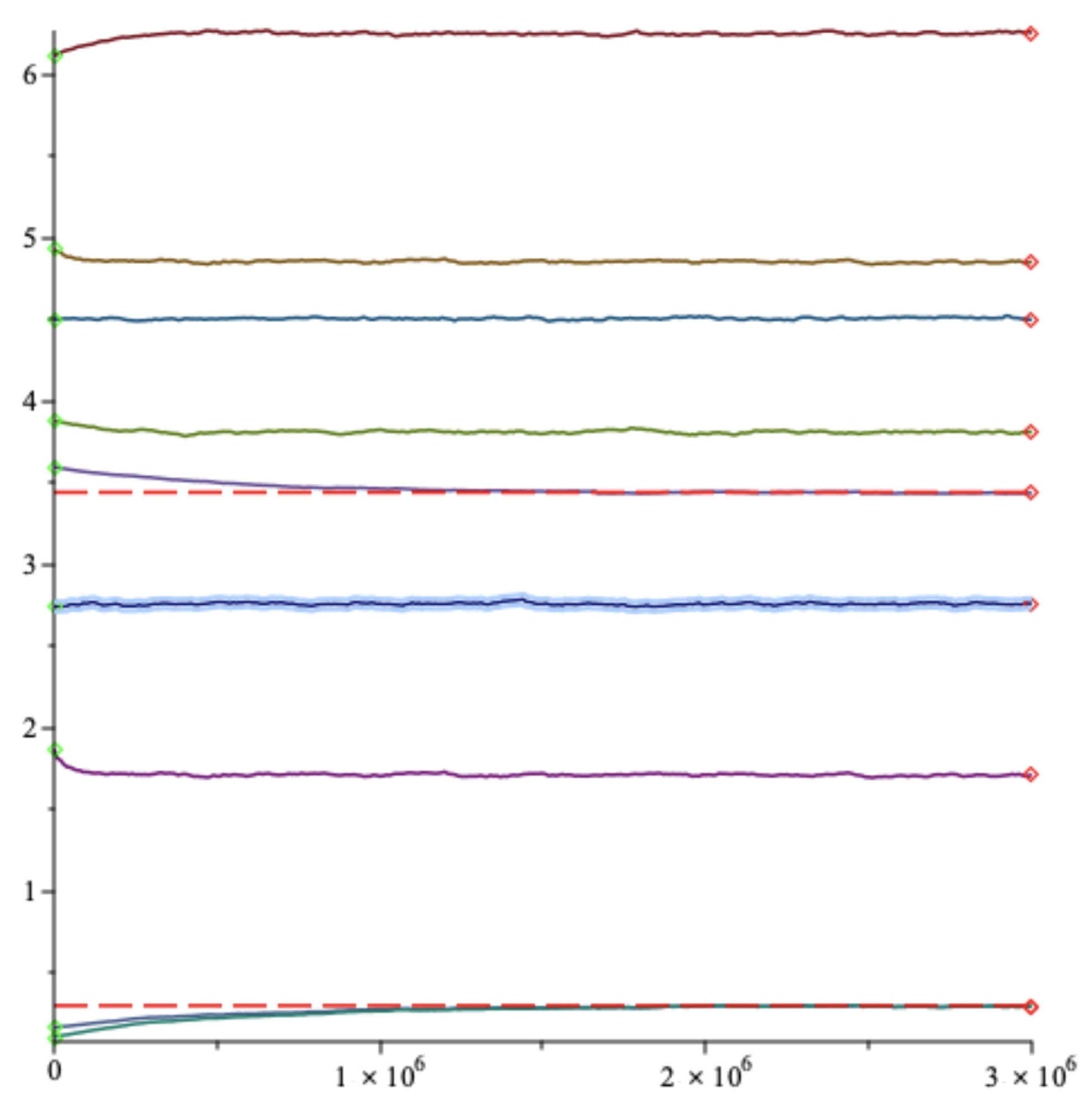
In Figure 1 we display our simulations as a sequence starting with a random initial . We assume that for all t the transmitted bit is always 0 i.e., the polarization angle is always . The learning rate is . We simulate nine parallel gradient descents randomly initialized sharing the same random feature sequence , with T = 3,000,000. On Figure 1 we plot the parallel evolutions of quantity . The initial points are green diamonds and the final points are red diamonds. Although we start with nine different positions, the trajectories converge toward . However, the convergence is slow, confirming the and worse rate. In fact, some initial positions converge even more slowly, and even after 3,000,000 trials, are still very far. The reason is that the target function has several local maxima as it is shown in Figure 2 where the belongs to the set of values for . It is very unlikely that a communication operator would tolerate so many runs (3,000,000) in order to have a proper convergence. However, it would be possible to run the gradient descents in parallel and act like with particle systems in order to select the fastest in convergence.
A supposedly faster gradient descent would be defined by the inverse derivative
We notice that in stationary situation (where we suppose that very little varies) we have which is equal to when . In Figure 3, we display our simulations as a sequence starting with a random initial . The learning rate is . We simulate nine parallel fast gradient descents randomly initialized sharing the same random feature sequence , with 3,000,000. The gradient descent converges fast but does not converge on the good value . Again it is due to the fact that the target function has several local maxima which act like a trap for the gradient descent.
5. Conclusions
We have presented a simple quantum tomography problem, the photon unknown polarization problem and have analyzed its learnability via AI over T runs. We have shown that the learning regret cannot decay faster than (i.e., a cumulative regret of ). Furthermore, the classic gradient descent is hampered by local extrema which may significantly impact the theoretical convergence rate.
Funding
This research received no external funding.
Institutional Review Board Statement
Not applicable.
Informed Consent Statement
Not applicable.
Data Availability Statement
Not applicable.
Conflicts of Interest
The author declares no conflict of interest.
References
- Tishby, N.; Zaslavsky, N. Deep learning and the information bottleneck principle. In Proceedings of the 2015 IEEE Information Theory Workshop (ITW), Jerusalem, Israel, 26 April–1 May 2015. [Google Scholar]
- Bouillard, A.; Jacquet, P. Quasi Black Hole Effect of Gradient Descent in Large Dimension: Consequence on Neural Network Learning. In Proceedings of the ICASSP 2019—2019 IEEE International Conference on Acoustics, Speech and Signal Processing (ICASSP), Brighton, UK, 12–17 May 2019. [Google Scholar]
- Abbe, E.; Sandon, C. Provable limitations of deep learning. arXiv 2018, arXiv:1812.06369. [Google Scholar]
- Ben-David, S.; Hrubeš, P.; Moran, S.; Shpilka, A.; Yehudayoff, A. Learnability can be undecidable. Nat. Mach. Intell. 2019, 1, 44–48. [Google Scholar] [CrossRef]
- Jacquet, P.; Shamir, G.; Szpankowski, W. Precise Minimax Regret for Logistic Regression with Categorical Feature Values. In Algorithmic Learning Theory; PMLR: New York City, NY, USA, 2021. [Google Scholar]
- Van Erven, T.; Harremos, P. Rényi divergence and Kullback–Leibler divergence. IEEE Trans. Inf. Theory 2014, 60, 3797–3820. [Google Scholar] [CrossRef]
- O’shea, T.; Hoydis, J. An introduction to deep learning for the physical layer. IEEE Trans. Cogn. Commun. Netw. 2017, 3, 563–575. [Google Scholar] [CrossRef] [Green Version]
- Newey, W.K.; McFadden, D. Chapter 36: Large sample estimation and hypothesis testing. In Handbook of Econometrics; Elsevier: Amsterdam, The Netherlands, 1994. [Google Scholar]
- Shtarkov, Y.M. Universal sequential coding of single messages. Probl. Inf. Transm. 1987, 23, 3–17. [Google Scholar]
Figure 1.
Angle estimate versus time of nine slow gradient descents randomly initialized. Green diamonds are starting points, red diamonds are stopping points.
Figure 1.
Angle estimate versus time of nine slow gradient descents randomly initialized. Green diamonds are starting points, red diamonds are stopping points.

Figure 2.
Target function as function of .

Figure 3.
Angle estimate versus time of nine fast gradient descents randomly initialized. Green diamonds are starting points, red diamonds are stopping points.
Figure 3.
Angle estimate versus time of nine fast gradient descents randomly initialized. Green diamonds are starting points, red diamonds are stopping points.

Disclaimer/Publisher’s Note: The statements, opinions and data contained in all publications are solely those of the individual author(s) and contributor(s) and not of MDPI and/or the editor(s). MDPI and/or the editor(s) disclaim responsibility for any injury to people or property resulting from any ideas, methods, instructions or products referred to in the content. |
© 2023 by the author. Licensee MDPI, Basel, Switzerland. This article is an open access article distributed under the terms and conditions of the Creative Commons Attribution (CC BY) license (https://creativecommons.org/licenses/by/4.0/).
Share and Cite
MDPI and ACS Style
Jacquet, P. Is Quantum Tomography a Difficult Problem for Machine Learning? Phys. Sci. Forum 2022, 5, 47. https://doi.org/10.3390/psf2022005047
AMA Style
Jacquet P. Is Quantum Tomography a Difficult Problem for Machine Learning? Physical Sciences Forum. 2022; 5(1):47. https://doi.org/10.3390/psf2022005047
Chicago/Turabian StyleJacquet, Philippe. 2022. "Is Quantum Tomography a Difficult Problem for Machine Learning?" Physical Sciences Forum 5, no. 1: 47. https://doi.org/10.3390/psf2022005047