A Computational Model to Determine Membrane Ionic Conductance Using Electroencephalography in Epilepsy ^†

Abstract

Epilepsy is a multiscale disease in which small alterations at the cellular scale affect the electroencephalogram (EEG). We use a computational model to bridge the cellular scale to EEG by evaluating the ionic conductance of the Hodkin–Huxley (HH) membrane model and comparing the EEG in response to intermittent photic stimulation (IPS) for epilepsy and normal subjects. Modeling is sectioned into IPS encoding, determination of an LTI system, and modifying ionic conductance to generate epilepsy signals. Machine learning is employed where it results in 0.6 $\left(\frac{\mathrm{mS}}{{\mathrm{cm}}^2}\right)$ ionic conductance in epilepsy. This ionic conductance is lower than the unitary conductance for normal subjects.

1. Introduction

Epilepsy is a chronic neurological disorder leading patients to experience recurrent seizures. Although the causes of epilepsy are reported in categories: structural, genetic, infectious, metabolic, immune, and unknown. The epilepsy mechanism is not fully understood. The diagnoses of epilepsy are basically clarified by an epileptologist based on clinical assessment and neuroimaging, as well as visual detection of interictal epileptiform discharges (IED)s which appeared in 30% of cases in their electroencephalography (EEG) signals [1]. EEG reveals a general overview of neuronal activity in disparate cortical regions by representing the potential difference between certain areas of the brain and a determined reference on the head surface in timeseries data [2]. Anti-seizure drugs (ASD)s are advised to control seizures, whereas surgery to remove the brain-affected region is the best option for the treatment of epilepsy. The risk of seizure decreases by 50% after surgery, which opens the door for fundamental research on the cellular scale [3]. Animal studies are expensive and enforces the employment of non-invasive techniques for solving the inverse problem. The question is how to solve EEG inverse problems towards discovering the intracranial information on the cellular scale involved with epilepsy.

Literature papers can be divided into two environments: molecular, cellular, and network scales; and cortical region-brain scales [4]. Simulators such as low-resolution brain electromagnetic tomography (LORETA) and BrainStorm are examples of studies that mainly use non-invasive techniques, e.g., fMRI and EEG; however, they rely on the neurophysiology achievements resulting from lower scale research [5,6,7]. In these simulators, the results of studies on lower scales are considered as the primary concept for the model, assisted by mathematics, physics, electronics, etc., towards proposing a higher scale model resulting in probable source localization. Although discovering the seizure onset zone (SOZ) in epilepsy studies using simulators are valuable, recurrent seizure after surgery still left the technique’s controversy. Studies reported that epileptic seizures may arise from the spread of cortical microdomains and influence the regions which are located further than the SOZ [8]. On a cellular scale, it is reported that the seizure originally comes from an impairment in balancing between excitatory and inhibitory synapses in epileptic seizure occurrence [9]. Moreover, the action potential is engaged with the synaptic activities in the membrane [10].

Stimulation by IPS as the common or routine epilepsy diagnostic method has become a golden method to trigger and distinguish the difference between case and control groups in EEG analysis (Kasteleijn-Nolst Trenité et al., 1987); albeit, it differed from one person to another [11]. On the cellular scale, IPS with a linkage with photoreceptors is dedicated to being connected to glutamate and then to the excitatory transmitter [12] towards a probable generating action potential [13]. Kerr et al. [14] applied the half-realistic half-abstract model of the thalamo-cortico-thalamic circuit in the cortical region proposed by Robinson et al. [15] for analyzing responses to simple visual stimuli; from the retina to the membrane.

In this paper, we propose a computational model to evaluate a rate of ionic conductance as one of the main parameters in the Hodgkin–Huxley (HH) realistic membrane model, in epilepsy compared to normal by analyzing EEG signals responded to IPS. IPS is used to provide a common condition for introducing a comparison of intracranial value between groups due to the limitation of accessibility to the actual value. The model is not only significant due to being an affordable solution in bridging cellular scale to EEG, but also it can be used to generate semi-EEG-oscillations. Figure 1 illustrates an overview of the study.

2. Materials and Methods

2.1. Dataset

In this study, retrospective data (65 epilepsy and 65 normal subjects) were collected from subjects who visited the Neuro Clinic of HCTM, Universiti Kebangsaan Malaysia (UKM) from 2019 to 2021. The categorization of case and control groups was based on the EEG reports and patients’ clinical profile, evidenced by diffuse generalized cerebral disturbance in the epilepsy group (who were taking 400–2500 milligrams of sodium valproate per day), and normal EEG with non-epilepsy illness as the normal group. For the measurement of EEG signals, subjects (male and female; age: 36.90 ± 13.40) were prepared to contain a contact impedance less than 5 kΩ and recorded at a 500 Hz sample rate based on a 10–20 standard EEG recording placement system. In this study, we only used the EEG section that responded to 18 Hz IPS acquired from the left primary visual cortex (O1) [16].

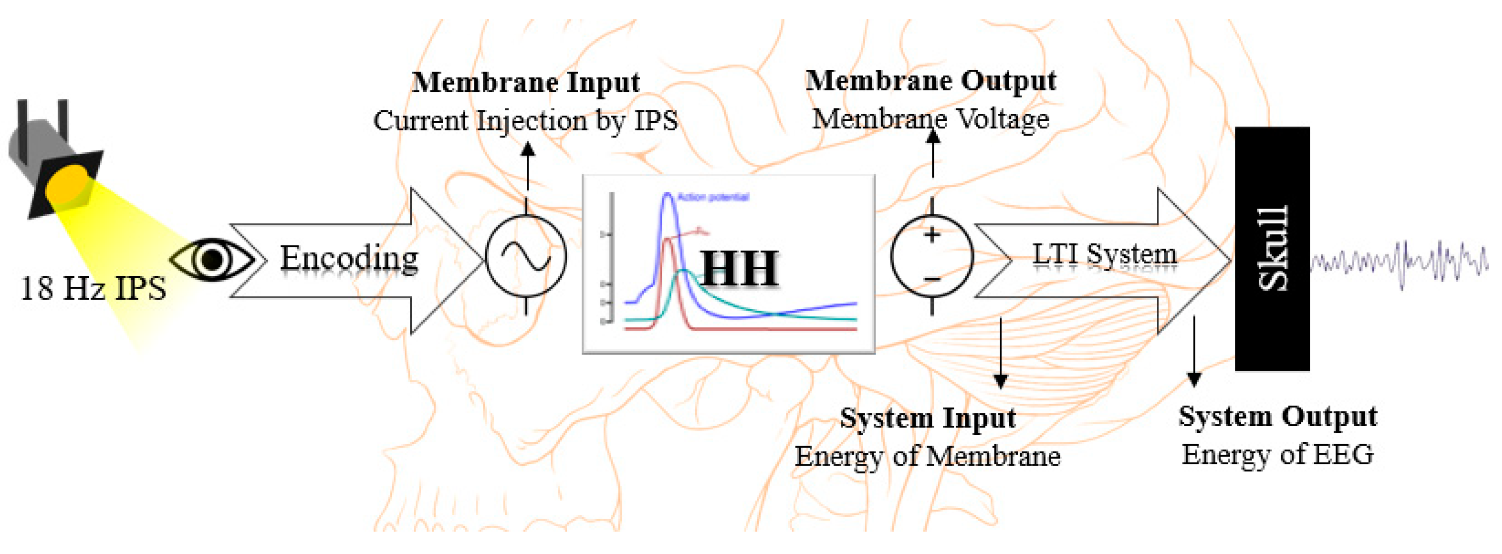
2.2. Hodgkin–Huxley Membrane Model Implementation

The Hodgkin–Huxley (HH) model is a mathematical model in a realistic environment that describes how an action potential is initiated and propagated [17]. Equation (1) is the main HH equation where $I$ is the current passing through the membrane, $C_m$ is membrane capacitance equal to 1 µF/cm². The model consists of three trajectories belonging to sodium, potassium, and leakage. $V_k$ and $V_N$ are potassium and sodium reversal potential equal to −77 mV and 50 mV, respectively. ${\overline{g}}_k$ is maximal potassium conductance equal to 36 mS/cm², whereas ${\overline{g}}_N$ is maximal sodium conductance equal to 120 mS/cm². ${\overline{g}}_l$ and ${\overline{V}}_l$ are the leak conductance per unit area and leak reversal potential. The values of $n^4$ and $m^3$ are the constant ratio of activated and inactivated gates for potassium and sodium, respectively. In the formula, $\left(V_m-V_k\right)$ and $\left(V_m-V_N\right)$ are the driving forces for potassium and sodium, respectively. They act as gears for adjusting and balancing the force of the membrane [18]. Whereas $T$ represents the ionic conductance for both sodium and potassium in the membrane.

$$I_m=C_m\frac{d_{V_m}}{d_t}+T({\overline{g}}_k{n}^4\left(V_m-V_k\right)+{\overline{g}}_{Na}{m}^{3}h\left(V_m-V_{Na}\right)+{\overline{g}}_l\left(V_m-V_l\right)$$

(1)

$C_m\frac{d_{V_m}}{d_t}$ refers to the membrane input current that plays the key role in the process of current injection [19]. The drawback relates to the lack of a principled method for determining the intensity of injection; hence, studies introduced different agreements [20]. Therefore, encoding IPS was essential.

2.3. Encoding Process of Intermittent Photic Stimulation

The encoding process translates IPS as extracranial stimulation to the current injecting of the cell. In this study, DC with 18 Hz frequency in one second has been used due to resulting in the best discrimination between the case and control [16]. In addition, the low and high values of the current injection must be determined. The low limit (during resting time) and high limit (during IPS) of DC have been determined experimentally depending on the membrane voltage spiking; regular or fast-spiking, respectively [21,22]. In this study, 1 to 10 µA and 2 to 100 µA have been examined with 1 resolution for low and high limitation, respectively. The first and the lowest values have been chosen as the low limit whereas the highest value has been chosen as the high limit.

2.4. Energy Calculation and Principle Linear Time Invariant System

The released membrane energy due to IPS has been calculated based on the relation between power and energy considering the value of output membrane voltage and membrane current. On the other side, the energy of EEG side is calculated according to the relation between power and energy considering the value of skull resistance and EEG potential differences due to 18 Hz IPS. The continuous-time transfer function (TF) in the LTI system has been used in the process of energy transmission followed by down-sampling from 100,000 to 500 (similar to the EEG sample rate) to cover the difference in time resolutions. The challenge refers to discovering one segment of the EEG signal (1 out of 10). The values of poles and zeros have been evaluated experimentally between 1 and 10 targeting energy of normal EEG signals. Each TF resulting from each value for pole and zero is determined using system identification toolbox in MATLAB based on the options; the initialization method using the instrumental variable (IV) algorithm, auto initial condition, no regularization, 20 iterations, 0.01 as tolerance and zero as the error threshold for outliner penalty. The search method was nonlinear least squares with the automatically chosen line search method. The fit frequency range was 0 to 3.14 rad/s. The acceptance threshold for LTI systems has been considered by over 60% of estimated fitness between input (membrane energy) and output (energy of normal EEGs). In the next step, the average has been taken from the gain, first poles, and first zeros (separately for real and imaginary values) of all achieved normal LTI systems. The resulting single LTI system is called the principle LTI system which is going to be used as the reference. The ionic conductance of the HH model to reach the principle LTI system equals 1 ($T=1\left(\frac{\mathrm{mS}S}{{\mathrm{cm}}^2}\right)$).

2.5. Hodgkin–Huxley Model Parameter Modification

From the previous steps, the same ionic conductance did not result in the same LTI system for both normal and epilepsy groups. Therefore, ionic conductance has been modified experimentally (from 0.1 to 2.0 with 0.1 resolution testing) aiming at the epilepsy signals passing through the principle LTI system. The desire is for a resulting LTI system to be achieved by one of the tested rates of ionic conductance based on the lowest difference from the principle LTI system (in the aspect of gain, first pole, and first zero). The result of this step is discovering the nominated rate (s) of ionic conductance that had been responsible for generating epilepsy EEG signals.

3. Results and Discussion

3.1. Intermittent Photic Stimulation Encoding

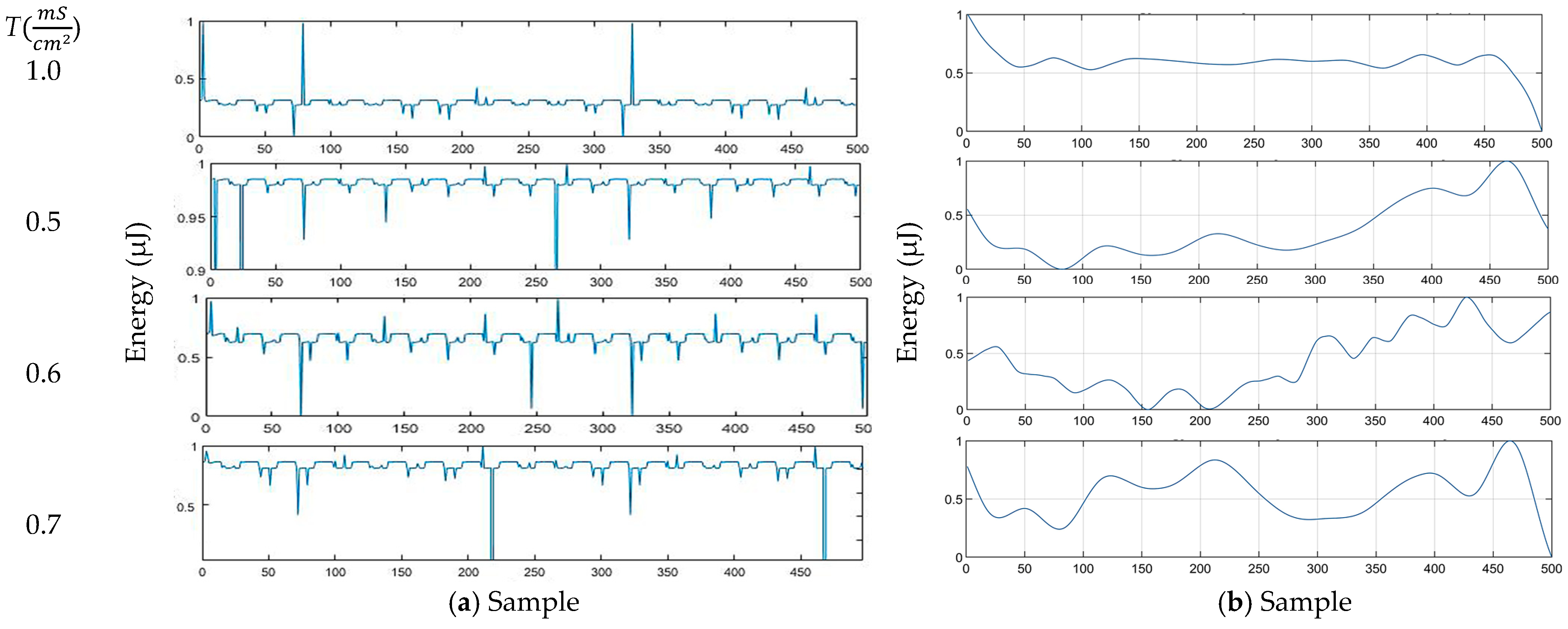
To transfer IPS to the injected value of the membrane, the encoding process focused on the 18 Hz frequency of IPS following discovering the low (3 µV) and the high limit (10 µV) DC as the best limitations for current injection. In Brunel et al. [23], the channel noise was performed under gaussian distribution and using the Markov chain model. Similarly, the research focused on synaptic noise and filtering the frequency response of spiking neurons. For a single membrane and DC injection, Rowat [24] compared the interspike interval distribution generated by a Markov chain model to the distribution generated by HH equations with current noise. Tuckwell [18] discussed theoretical neurobiology and went in-depth into stochastic theories following the Markov chain model.

3.2. Energy

Different types of energies, specifically at the cellular and molecular levels, were discussed. Calculating the Hamiltonian of a system which is an operator corresponding to the total energy of that system, including kinetic energy and potential energy, was performed, aimed at discovering the connection between energy and firing patterns in the Hindmarch–Rose neuron model [25]. Usha et al. [26] measured the metabolic energy which is required to maintain the stability of the HH neuron model in fast-spiking mode, exposing an external electric field. The presence of the electric field increases the membrane potential, electrical energy supply, and metabolic energy consumption were reported. In our study, the “energy” reflects the electrical energy by assuming the cell as an electrical system with the note that it comes from chemical charges [27].

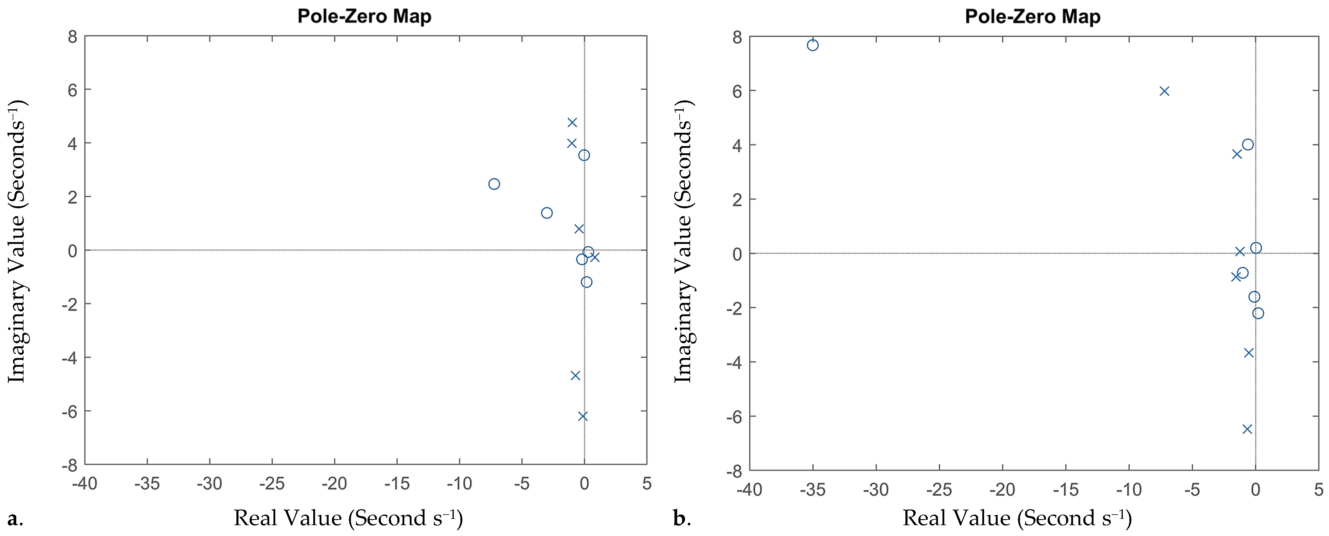
3.3. Principle Linear Time Invariant System

The result shows that the membrane energy (with ($T=1 \left(\frac{\mathrm{mS}S}{{\mathrm{cm}}^2}\right)$) is transferred to the energy of the fourth segment of normal EEG through the Equation (2); with six poles and six zeros.

Table 1. A comparison between normal (Principle) and epilepsy LTI systems with the same ionic conductance.

Gain	Normal	−0.8401
	Epilepsy	−0.06001
		First	Second	Third	Fourth	Fifth	Sixth
Zero	Normal	−7.23 + 2.464i	−3.01 + 1.385i	−0.033 + 3.54i	0.3002 − 0.072i	0.1672 − 1.193i	−0.201 − 0.345i
	Epilepsy	−35.01 + 7.67i	−0.61 + 4.01i	−0.102 − 1.602i	0.031 + 0.2012i	0.201 − 2.21i	−1.021 − 0.72i
Pole	Normal	−0.98 + 4.76i	−1.01 + 3.983i	−0.12 − 6.204i	−0.72 − 4.68i	−0.43 + 0.79i	0.83 − 0.27i
	Epilepsy	−7.206 + 5.98i	−0.65 − 6.478i	−1.47 + 3.659i	−0.543 − 3.67i	−1.23 + 0.067i	−1.56 − 0.87i

represents a comparison between the principle and epilepsy LTI system with the same ionic conductance in the aspect of gain, zeros, and poles based on complex numbers. It shows that the first poles and zeros represent the most difference between groups compared to the rest values. Figure 2 shows the pole-zero map of the principle (a) and epilepsy (b) LTI system with $T=1 \left(\frac{\mathrm{mS}S}{{\mathrm{cm}}^2}\right)$. According to the definitions, the principle LTI system is stable and compared to the epilepsy system, it is in addition to being a faster response that contains more oscillations.

$$F_N\left(s\right)=\frac{-0.06001 \left(s-\left(0.3002-0.072i)\right)\left(s+\left(0.201+0.345i\right)\right)\left(s-\left(0.1672-1.193i\right)\right)\left(s+3.01-1.385i\right)\right)\left(s+7.23-2.464i\right))\left(s+\left(0.033-3.54i\right)\right)}{\left(s-\left(0.83-0.27i\right)\right)\left(s+0.43-0.79i\right))\left(s+1.01-3.983i\right))\left(s+0.72+4.68i\right))\left(s+\left(0.98-4.76i\right)\right)\left(s+\left(0.12+6.204i\right)\right)}$$

(2)

The reason the fourth segment (approximately middle of 10 s) was the best in modeling may be due to the neural entrainment due to synchronization of neural activity with the periodic properties of the stimuli [28,29,30]. This issue is out of the scope of this study which requires invasive and in-depth analysis and measurements in vivo. In Rosa et al. [31], an LTI system with a focus on TF was used to transfer neuronal activity to the blood oxygen level dependency (BOLD) factor using simultaneous EEG-fMRI. The responses due to visual stimulation were computed by the first segment in a half-second (500 ms) of EEG data (left occipital) acquired from inside the MRI scanner. Then they took the average of the results from all subjects.

To select the right orders in the system identification step, in Fabri et al. [32] the orders were selected arbitrarily in a movement control of the brain–computer interface (BCI) study that focused on parametric modeling of EEG with six poles and two zeros. In another EEG study, Narasimhan [33] dealt with the pole-zero spectral modeling of EEG by methods based on homomorphic filtering and linear prediction. Although the manner of choosing orders in our study was performed based on reaching over 60% fitness estimation as the initial target fitness, further investigation with a higher threshold can be considered.

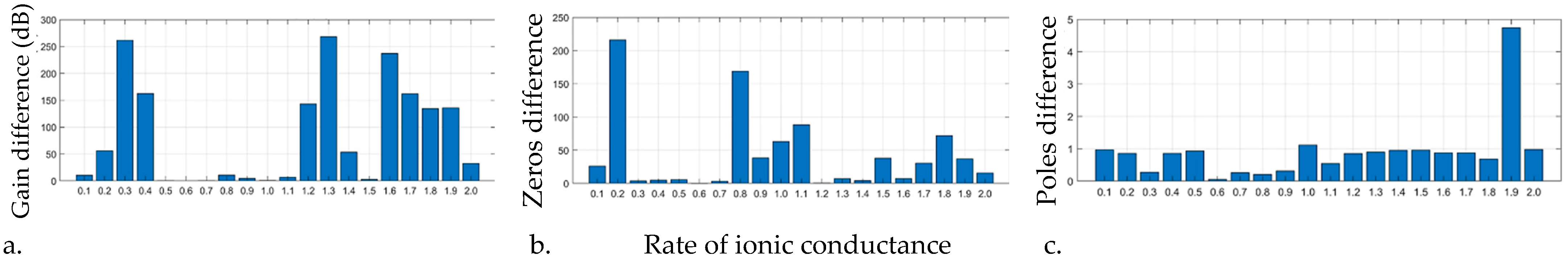
3.4. Rates of Ionic Conductance in Epilepsy

Different tested rates of ionic conductance led to achieving different epilepsy LTI systems. The minimum difference in gain, first pole, and zero from the values in the principle LTI system brought us to the nominated rate(s) of ionic conductance for epilepsy. Figure 3 depicts the difference between epilepsy LTI systems obtained from different ionic condutance and principle LTI systems. According to Figure 3a, based on the threshold (<0.8 dB), the values remained 0.5, 0.6, 0.7, 1.1, and 1.5 (dB). Furthermore, considering Figure 3b,c, 1.1 and 1.5 must be excluded. Eventually, we kept 0.5, 0.6, and 0.7 as the rates of conductance as nominated values for the epilepsy group.

3.5. Simulation Signals and Filtering

Figure 4 shows samples of the raw and filtered simulated signals obtained from nominated rates of conductance. In this figure, DWT was applied to filter each simulated signal towards making them smooth. The figures show a slightly smoother signal than normal and the similarity with the signal achieved by a 0.5 rate of ionic conductance. In contrast, harsh frequency and higher amplitude compared to normal signal are observed in the signal from a 0.6 rate whereas the signal with 0.7 follows the frequency of a normal signal even though the amplitude is different. By now, we can expect 0.6 as the rate of ionic conductance for epilepsy. However, machine learning is one of the methods that assist to do the comparison accurately. In this stage, we train the classification model using the actual energy of EEG signals and test by simulated signals towards reaching the well-classified simulated signal generated from the particular truthful rate of ionic conductance.

3.6. Test and Validation

3.6.1. Feature Extraction and Feature Dimensionality Reduction

We extracted features from actual data (energy of EEG signals) in the training stage. Fifteen features have been extracted from the time and frequency domain from the fourth segment of actual data. In the time domain is the mean, median, standard deviation (STD), minimum, maximum, peak to peak (P to P), kurtosis (Kurt), skewness (Skew), root mean square (RMS), peak to RMS (P to RMS), root sum square (RSS). In the frequency domain is the delta, theta, alpha, and beta frequency bands. Next, the correlation coefficients for all features and the p-value have been achieved using the paired t-test. We dropped out the features that were highly correlated and then included only one of them besides the low-correlated ones. In the end, there are three possible groups of features that have been selected.

3.6.2. Classification Model Performance

Table 2. Performance of three different optimized SVM models using selected features in training and testing stages.

Training						Testing	Rates of Ionic Conductance
	Features	Classifier	Acc	Sen	Spc		1	0.5	0.6	0.7
	Kurt, P2P	Opt SVM	80.6%	78.5%	81.04%		✓	✗	✓	✓
	Kurt, P2P, Alpha	Opt SVM	82.1%	89.2%	78.3%		✓	✗	✓	✗
	Skew, RSS	Opt SVM	81.3%	71.08%	69.84%		✓	✗	✓	✗

represents the performance of three different optimized SVM models using various selected features in the training stage and the result of the testing stage for nominated rates of ionic conductance. The results show that 1 and 0.6 as the rate of ionic conductance for normal and epilepsy successfully classified the EEG as normal and epilepsy, respectively, using all models. This shows epilepsy signals have a lower rate of ionic conductance compared to normal signals reaching 18 Hz IPS. The lower rate of ionic conductance is also confirmed by Groppa et al. [34] in generalized epilepsy and IPS study, where they served lower activation of excitatory neurotransmitters and higher inhibitory due to IPS. The literature shows a boosting of the level of glutamate as the excitatory neurotransmitter by IPS following the firing of the neuron, increasing ionic congestion and increasing the ionic conductivity [4]. On the other side, a rise in the level of glutamate during ictal is reported [35] following increasing ionic congestion and conductivity. It seems that photic stimulation and seizure trace the same scenario [4,12]. However, we investigated EEG data during interictal and the IPS on a cellular scale was performed in normal samples. Therefore, we could not expect IPS and interictal results (increasing ionic conductance) in our research.

In our study, EEG recoding was in the condition when all epileptic subjects had been medically advised to take ASDs. Going in-depth into the efficacy of ASD on cells and the membrane, the ASDs have the effect of blocking the excitatory receptors [36] which could affect our result by lowering the ionic conductance in epilepsy signals. Furthermore, in some studies, to prevent the generation of seizures, they even worked on blocking glutamate transporters [37]. Moreover, one of the hypotheses in seizure generation reported the progressive intracellular sodium insertion which is directly related to the ionic conductance [38].

4. Conclusions

The results of this study show that the proposed model using the HH membrane model and testing EEG data in the presence of IPS is a promising tool for discovering the comparative rate of ionic conductance between the normal and epilepsy EEG signals. The study represents a computational model to solve the brain inverse problem through bridging cellular scale and EEG signals in the study of epilepsy. Despite the high complexity of computation, the model is a low-cost solution in a human study to reach the cellular information using EEG signals compared to high-cost invasive techniques.

References

1. Renzel, R.; Tschaler, L.; Mothersill, I.; Imbach, L.L.; Poryazova, R. Sensitivity of long-term EEG monitoring as a second diagnostic step in the initial diagnosis of epilepsy. Epileptic Disord. 2021, 23, 572–578. [Google Scholar] [CrossRef]
2. Olejniczak, P. Neurophysiologic basis of EEG. J. Clin. Neurophysiol. 2006, 23, 186–189. [Google Scholar] [CrossRef] [PubMed]
3. Zhang, L.; Jiang, X.-Y.; Zhou, D.; Zhang, H.; Bao, S.-M.; Li, J.-M. Postoperative seizure outcome and timing interval to start antiepileptic drug withdrawal: A retrospective observational study of non-neoplastic drug resistant epilepsy. Sci. Rep. 2018, 8, 13782. [Google Scholar] [CrossRef] [PubMed]
4. Biedermann, J.; Braunbeck, S.; Plested, A.J.R.; Sun, H. Nonselective cation permeation in an AMPA-type glutamate receptor. Proc. Natl. Acad. Sci. USA 2021, 118, e2012843118. [Google Scholar] [CrossRef] [PubMed]
5. Worrell, G.A.; Lagerlund, T.D.; Sharbrough, F.W.; Brinkmann, B.H.; Busacker, N.E.; Cicora, K.M.; O’Brien, T.J. Localization of the epileptic focus by low-resolution electromagnetic tomography in patients with a lesion demonstrated by MRI. Brain Topogr. 2000, 12, 273–282. [Google Scholar] [CrossRef]
6. Tadel, F.; Baillet, S.; Mosher, J.C.; Pantazis, D.; Leahy, R.M. Brainstorm: A User-Friendly Application for MEG/EEG Analysis. Comput. Intell. Neurosci. 2011, 2011, 879716. [Google Scholar] [CrossRef]
7. Grech, R.; Cassar, T.; Muscat, J.; Camilleri, K.P.; Fabri, S.G.; Zervakis, M.; Xanthopoulos, P.; Sakkalis, V.; Vanrumste, B. Review on solving the inverse problem in EEG source analysis. J. Neuroeng. Rehabil. 2008, 5, 25. [Google Scholar] [CrossRef]
8. Gao, F.; Song, X.; Zhu, D.; Wang, X.; Hao, A.; Nadler, J.V.; Zhan, R.Z. Dendritic morphology, synaptic transmission, and activity of mature granule cells born following pilocarpine-induced status epilepticus in the rat. Front. Cell. Neurosci. 2015, 9, 384. [Google Scholar] [CrossRef]
9. Sun, H.; Takesian, A.E.; Wang, T.T.; Lippman-Bell, J.J.; Hensch, T.K.; Jensen, F.E. Early Seizures Prematurely Unsilence Auditory Synapses to Disrupt Thalamocortical Critical Period Plasticity. Cell Rep. 2018, 23, 2533–2540. [Google Scholar] [CrossRef]
10. Faber, D.S.; Pereda, A.E. Two Forms of Electrical Transmission Between Neurons. Front. Mol. Neurosci. 2018, 11, 427. [Google Scholar] [CrossRef]
11. Aminoff, M.J. Aminoff’s Electrodiagnosis in Clinical Neurology, 6th ed.; Elsevier Inc.: Amsterdam, The Netherlands, 2012; ISBN 978-1-4557-0308-1. [Google Scholar]
12. Rose, C.R.; Felix, L.; Zeug, A.; Dietrich, D.; Reiner, A.; Henneberger, C. Astroglial Glutamate Signaling and Uptake in the Hippocampus. Front. Mol. Neurosci. 2018, 10, 451. [Google Scholar] [CrossRef] [PubMed]
13. Miyachi, E.-I.; Kawai, F. Voltage-Gated Ion Channels in Human Photoreceptors: Na+ and Hyperpolarization-Activated Cation Channels. In The Neural Basis of Early Vision; Kaneko, A., Ed.; Springer: Tokyo, Japan, 2003; ISBN 978-4-431-68449-7. [Google Scholar]
14. Kerr, C.C.; Rennie, C.J.; Robinson, P.A. Physiology-based modeling of cortical auditory evoked potentials. Biol. Cybern. 2008, 98, 171–184. [Google Scholar] [CrossRef] [PubMed]
15. Robinson, P.A.; Rennie, C.J.; Rowe, D.L.; O’Connor, S.C.; Gordon, E. Multiscale brain modelling. Philos. Trans. R. Soc. B Biol. Sci. 2005, 360, 1043–1050. [Google Scholar] [CrossRef]
16. Najafi, T.; Jaafar, R.; Remli, R.; Zaidi Wan, A.W.; Chellappan, K. Brain Dynamics in Response to Intermittent Photic Stimulation in Epilepsy. Int. J. Online Biomed. Eng. 2022, 18, 80–95. [Google Scholar] [CrossRef]
17. Hodgkin, A.L.; Huxley, A.F. A quantitative description of membrane current and its application to conduction and excitation in nerve. J. Physiol. 1952, 117, 500–544. [Google Scholar] [CrossRef]
18. Tuckwell, H.C. Introduction to Theoretical Neurobiology; Cambridge Studies in Mathematical Biology; Cambridge University Press: Cambridge, UK, 1988; Volume 2. [Google Scholar] [CrossRef]
19. Goldwyn, J.H.; Shea-Brown, E. The what and where of adding channel noise to the Hodgkin-Huxley equations. PLoS Comput. Biol. 2011, 7, e1002247. [Google Scholar] [CrossRef]
20. Zhang, Y.; Wang, K.; Yuan, Y.; Sui, D.; Zhang, H. Effects of Maximal Sodium and Potassium Conductance on the Stability of Hodgkin-Huxley Model. Comput. Math. Methods Med. 2014, 2014, 761907. [Google Scholar] [CrossRef] [PubMed]
21. Bhattacharya, B.S.; Patterson, C.; Galluppi, F.; Durrant, S.J.; Furber, S. Engineering a thalamo-cortico-thalamic circuit on spinnaker: A preliminary study toward modeling sleep and wakefulness. Front. Neural Circuits 2014, 8, 46. [Google Scholar] [CrossRef]
22. Skinner, F.K. Moving beyond Type I and Type II neuron types. F1000Research 2013, 2, 19. [Google Scholar] [CrossRef] [PubMed]
23. Brunel, N.; Chance, F.S.; Fourcaud, N.; Abbott, L.F. Effects of synaptic noise and filtering on the frequency response of spiking neurons. Phys. Rev. Lett. 2001, 86, 2186–2189. [Google Scholar] [CrossRef] [PubMed]
24. Rowat, P. Interspike interval statistics in the stochastic Hodgkin-Huxley model: Coexistence of gamma frequency bursts and highly irregular firing. Neural Comput. 2007, 19, 1215–1250. [Google Scholar] [CrossRef] [PubMed]
25. Xu, L.; Qi, G.; Ma, J. Modeling of memristor-based Hindmarsh-Rose neuron and its dynamical analyses using energy method. Appl. Math. Model. 2022, 101, 503–516. [Google Scholar] [CrossRef]
26. Usha, K.; Sreepriya, M.K.; Subha, P.A. Energy consumption in Hodgkin–Huxley type fast spiking neuron model exposed to an external electric field. Perspect. Sci. 2016, 8, 132–134. [Google Scholar] [CrossRef]
27. Grider, M.H.; Jessu, R.; Kabir, R. Physiology, Action Potential; Springer Nature: Treasure Island, FL, USA, 2022. [Google Scholar]
28. Graaf, D.; De Graaf, T.A.; Gross, J.; Paterson, G.; Rusch, T.; Sack, A.T.; Thut, G. Alpha-Band Rhythms in Visual Task Performance: Phase- Locking by Rhythmic Sensory Stimulation. PLoS ONE 2013, 8, e60035. [Google Scholar] [CrossRef] [PubMed]
29. Mathewson, K.E.; Basak, C.; Maclin, E.L.; Low, K.A.; Boot, W.R.; Kramer, A.F.; Fabiani, M.; Gratton, G. Different slopes for different folks: Alpha and delta EEG power predict subsequent video game learning rate and improvements in cognitive control tasks. Psychophysiology 2012, 49, 1558–1570. [Google Scholar] [CrossRef] [PubMed]
30. Thut, G.; Schyns, P.G.; Gross, J.; Rosenblum, M. Entrainment of perceptually relevant brain oscillations by non-invasive rhythmic stimulation of the human brain. Front. Psychol. 2011, 2, 170. [Google Scholar] [CrossRef]
31. Rosa, M.J.; Kilner, J.; Blankenburg, F.; Josephs, O.; Penny, W. Estimating the transfer function from neuronal activity to BOLD using simultaneous EEG-fMRI. Neuroimage 2010, 49, 1496–1509. [Google Scholar] [CrossRef]
32. Fabri, G.S.; Camilleri, K.P.; Cassar, T. Parametric Modelling of EEG Data for the Identification of Mental Tasks. In Biomedical Engineering, Trends in Electronics, Communications and Software; IntechOpen: London, UK, 2011. [Google Scholar]
33. Narasimhan, S.V. Pole-zero spectral modeling of EEG. Signal Process. 1989, 18, 17–32. [Google Scholar] [CrossRef]
34. Groppa, S.; Siebner, H.R.; Kurth, C.; Stephani, U.; Siniatchkin, M. Abnormal response of motor cortex to photic stimulation in idiopathic generalized epilepsy. Epilepsia 2008, 49, 2022–2029. [Google Scholar] [CrossRef]
35. Barker-Haliski, M.; Steve White, H. Glutamatergic mechanisms associated with seizures and epilepsy. Cold Spring Harb. Perspect. Med. 2015, 5, a022863. [Google Scholar] [CrossRef]
36. Czapiński, P.; Blaszczyk, B.; Czuczwar, S.J. Mechanisms of action of antiepileptic drugs. Curr. Top. Med. Chem. 2005, 5, 3–14. [Google Scholar] [CrossRef] [PubMed]
37. Demarque, M.; Villeneuve, N.; Manent, J.-B.; Becq, H.; Represa, A.; Ben-Ari, Y.; Aniksztejn, L. Glutamate transporters prevent the generation of seizures in the developing rat neocortex. J. Neurosci. 2004, 24, 3289–3294. [Google Scholar] [CrossRef] [PubMed]
38. Raimondo, J.V.; Burman, R.J.; Katz, A.A.; Akerman, C.J. Ion dynamics during seizures. Front. Cell. Neurosci. 2015, 9, 419. [Google Scholar] [CrossRef] [PubMed] [Green Version]
Figure 1. An overview of study hypothesis.
Psf 05 00045 g001
Figure 2. Pole-zero plot of principle LTI system with ionic conductance equals to T = 1 ( mS S cm 2 ) .
Psf 05 00045 g002
Figure 3. Systems comparison with different rates of ionic conductance in the aspect of gain (a); first zero (b); and first pole (c).
Psf 05 00045 g003
Figure 4. Raw and filtered simulated signals obtained from nominated rates of conductance.
Psf 05 00045 g004