Analysis of Dynamical Field Inference in a Supersymmetric Theory ^†

Abstract

The inference of dynamical fields is of paramount importance in science, technology, and economics. Dynamical field inference can be based on information field theory and used to infer the evolution of fields in dynamical systems from finite data. Here, the partition function, as the central mathematical object of our investigation, invokes a Dirac delta function as well as a field-dependent functional determinant, which impede the inference. To tackle this problem, Fadeev–Popov ghosts and a Lagrange multiplier are introduced to represent the partition function by an integral over those fields. According to the supersymmetric theory of stochastics, the action associated with the partition function has a supersymmetry for those ghost and signal fields. In this context, the spontaneous breakdown of supersymmetry leads to chaotic behavior of the system. To demonstrate the impact of chaos, characterized by positive Lyapunov exponents, on the predictability of a system’s evolution, we show for the case of idealized linear dynamics that the dynamical growth rates of the fermionic ghost fields impact the uncertainty of the field inference. Finally, by establishing perturbative solutions to the inference problem associated with an idealized nonlinear system, using a Feynman diagrammatic expansion, we expose that the fermionic contributions, implementing the functional determinant, are key to obtain the correct posterior of the system.

1. Introduction

The evolution of some field of interest, called signal field, in a dynamical system described by a stochastic differential equation is not entirely determined by initial and boundary conditions but is excited by some stochastic field. These kind of dynamics play an important role not just in physics [1], but also in biology [2], chemistry [3], and economics [4,5] and can be based on imperfections in the model [6] or just an intrinsic stochastic behavior [7]. Here, we consider a measurement in the dynamical system, from which we can infer the current state and the evolution of a signal field using dynamical field inference (DFI). The base of DFI is information field theory (IFT), which is an information theory for fields within a Bayesian framework. DFI allows, in principle, to work with arbitrary stochastic differential equations to reconstruct a field, i.e., an infinite-dimensional signal, from some finite-dimensional measurement or other data. The reconstruction of a signal field in DFI exploits the prior knowledge on the signal properties, which are encoded in the stochastic differential equation. Nonlinearities in the stochastic differential equation lead to a complicated structure of the prior probability, which impedes the reconstruction of the corresponding signal field. Here, the central part of the investigation is the partition function. To cope with the problematic terms of the prior probability in the partition function, the supersymmetric theory of stochastics (STS) [8,9,10,11] introduces bosonic and fermionic ghost fields, which prove to obey a supersymmtry. In accordance with STS, we analyze this supersymmetry in the system from an IFT perspective. One of the major takeaways of STS is that the spontaneous breakdown of the observed supersymmetry leads to a chaotic behavior of the system. We show for two instructive examples of dynamical systems that chaos impacts the uncertainty of the field inference on a level that depends on the relevant system’s Lyapunov exponent.

2. Information Field Theory

In many areas of science, technology, and economics, the task of interpreting incomplete, noisy, and finite datasets arises [12,13]. Especially, if the quantity of interest is a field, there is an infinite number of possible signal field realizations that meet the constraints of a finite number of measurements. For such problems, which are called field inference problems, IFT was developed.

A physical field $\phi :\mathsf{\Omega }\to \mathbb{R}$ is a function that assigns a value to each point in time and u-dimensional position space. Here, the space and time will be handled in same the manner as in [14,15] and are denoted by the space-time location $x=(\overrightarrow{x},t)\in \mathsf{\Omega }={\mathbb{R}}^u\times {\mathbb{R}}_0^{+}$, $u\in \mathbb{N}$. For definiteness, we let the time axis start at $t_0=0$. As the field ${\phi }_x=\phi (x)$ has an infinite number of degrees of freedom, the integration is represented by path integrals over the integration measure $\mathcal{D}\phi ={\prod }_{x\in \mathsf{\Omega }}d{\phi }_x$ [16]. In the following, these space-time coordinate-dependent fields are denoted as abstract vectors in Hilbert space, such that the scalar product can be written as ${\gamma }^{†}\phi :=\int \mathrm{d}x{\gamma }^{*}(x)\phi (x)$, where ${}^{*}$ denotes the complex conjugate.

In order to get to know a field $\phi$, one has to measure it. Bayes’ theorem states how to update any existing knowledge given a finite number of measurement constraints. In this probabilistic logic, knowledge states are described by probability distributions. Accordingly, the prior knowledge $\mathcal{P}(\phi )$ is updated given a data vector d to the posterior probability [17]

$$\begin{array}{c}\hfill \mathcal{P}(\phi |d)=\frac{\mathcal{P}(d|\phi )\mathcal{P}(\phi )}{\mathcal{P}(d)}=\frac{\mathcal{P}(d|\phi )\mathcal{P}(\phi )}{\int \mathcal{D}\phi \mathcal{P}(d|\phi )\mathcal{P}(\phi )}.\end{array}$$

(1)

To construct the posterior, we need to have the prior $P(\phi )$ and the likelihood $\mathcal{P}(d|\phi )$. However, the evidence, $\mathcal{P}(d)$ is the normalization of the posterior and can be calculated from the prior and the likelihood. The prior probability of the signal, $\phi$, specifies the knowledge on the signal before any measurement, whereas the likelihood describes the measurement process. Any measurement process can be described by a response of an instrument R, which converts some discrete dataset to a continuous signal, and some additive noise n, $d=R[\phi ]+n$. The statistics of the noise then determine the likelihood. Particularly, if we assume Gaussian noise with known covariance N, we get

$$\begin{array}{c}\hfill \mathcal{P}(d|\phi )=\int \mathcal{D}n\mathcal{P}(d|n,\phi )\mathcal{P}(n|\phi )=\int \mathcal{D}n\delta (d-R[\phi ]-n)\mathcal{G}(n,N)=\mathcal{G}(d-R[\phi ],N).\end{array}$$

(2)

Here, we can also define initial conditions via initial data $d_0={\phi }_0=\phi (·,t_0)$. In this case, the response is defined as $R_0[\phi ]=\phi (·,t_0)$ and the noise vanishes, $\mathcal{P}(n)=\delta (n)$. Thus, the initial data likelihood is represented by $\mathcal{P}(d_0,\phi )=\mathcal{P}(d|\phi ,d_0=\phi (·,t_0))=\delta (\phi (·,t_0)-{\phi }_0)$ and can be combined with any data on the later evolution, $\tilde{d}$, via $\mathcal{P}(d|\phi )=\mathcal{P}(d_0|\phi )\mathcal{P}(\tilde{d}|\phi )$, with $d=(d_0,\tilde{d})$.

For the reconstruction, particularly the cumulants of first and second order are of interest, as they describe the mean, $m={\langle \phi \rangle }_{(\phi |d)}^c={\langle \phi \rangle }_{(\phi |d)}$, and the uncertainty dispersion, $D={\langle \phi {\phi }^{†}\rangle }_{(\phi |d)}^c:={\langle (\phi -m){(\phi -m)}^{†}\rangle }_{(\phi |d)}$. These posterior-connected correlation functions, or cumulants can be obtained via the moment-generating partition function ${\mathcal{Z}}_d[J]$,

$$\begin{array}{c}\hfill {\mathcal{Z}}_d[J]=\int \mathcal{D}\phi e^{-\mathcal{H}(d,\phi )+J^{†}}\to {\langle \phi (x_1)\dots \phi (x_n)\rangle }_{(\phi |d)}^c:=\frac{{\delta }^{n}log{\mathcal{Z}}_d[J]}{\delta J^{*}(x_1)\dots \delta J^{*}(x_n)}{|}_{J=0},\end{array}$$

(3)

where $\mathcal{H}(d,\phi ):=-ln(\mathcal{P}(d,\phi ))$ is the so-called information Hamiltonian.

3. Dynamical Field Inference

In DFI, a signal, for which we have prior information on the dynamics of the system, is inferred. In particular, we consider a signal which obeys a stochastic differential equation

$$\begin{array}{c}\hfill {\partial }_t\phi =F[\phi ](x)+\xi (x).\end{array}$$

(4)

The first part of the stochastic differential equation, ${\partial }_t\phi (x)=F[\phi ](x)$, describes the deterministic dynamics of the field and the excitation field, $\xi$, turns this deterministic evolution into a stochastic one. Here, the signal field, $\phi$, is defined for all $x\in \mathsf{\Omega }={\mathbb{R}}^u\times {\mathbb{R}}_0^{+}$, while ${\partial }_t\phi$ and $\xi$ live on ${\mathsf{\Omega }}^{\prime }={\mathbb{R}}^u\times {\mathbb{R}}^{+}$. Therefore, Equation (4) makes only statements about fields on ${\mathsf{\Omega }}^{\prime }$. Equation (4) can be summarized by an operator $\tilde{G}[\phi ]$, $\tilde{G}:{\mathcal{C}}^{n,1}(\mathsf{\Omega })\to \mathcal{C}({\mathsf{\Omega }}^{\prime })$, which contains all the time and space derivatives of the stochastic differential equation up to order n in space

$$\begin{array}{c}\hfill \tilde{G}[\phi ](x)=\xi (x)\mathrm{with}\tilde{G}[\phi ](x):={\partial }_t\phi (x)-F[\phi ](x),\end{array}$$

(5)

where $\tilde{\phi }=\phi (·,t\ne t_0)$ and $\phi =({\phi }_0,\tilde{\phi })$. In order to define the prior information given by the stochastic differential equation, we assume Gaussian statistics for the excitation field, $\mathcal{P}(\xi )=\mathcal{G}(\xi ,\mathrm{\Xi })$, with known covariance $\mathrm{\Xi }$. We define the combined vector of fields $\eta ={({\phi }_0,\xi )}^{†}$ that determines the dynamics with $\mathcal{P}(\eta )=\mathcal{P}({\phi }_0)\mathcal{G}(\xi ,\mathrm{\Xi })$ and extend the operator $\tilde{G}$ by the initial conditions to $G[\phi ]=({\phi }_0,\tilde{G}[\phi ])$ with $G:{\mathcal{C}}^{n,1}(\mathsf{\Omega })\to \mathcal{C}(\mathsf{\Omega })$ such that $G[\phi ]=\eta$. Assuming that there is a unique solution to the stochastic differential equation in Equation (5), the prior probability can be calculated via $\mathcal{P}(\phi |\eta )=\delta (\eta -G[\phi ])∥\frac{\delta \tilde{G}[\phi ]}{\delta \tilde{\phi }}∥$ as follows:

$$\begin{array}{c}\hfill \mathcal{P}(\phi )=\int \mathcal{D}\eta \mathcal{P}(\phi |\eta )\mathcal{P}(\eta )=\underset{=:\mathcal{B}(\phi )}{\underbrace{\frac{1}{\sqrt{|2\pi \mathrm{\Xi }|}}{e}^{-\frac{1}{2}\tilde{G}{[\phi ]}^{†}{\mathrm{\Xi }}^{-1}\tilde{G}[\phi ]}}}\underset{=:\mathcal{J}(\phi )}{\underbrace{∥\frac{\delta \tilde{G}[\phi ]}{\delta \tilde{\phi }}∥}}\mathcal{P}({\phi }_0),\end{array}$$

(6)

where $\delta \tilde{G}[\phi ]/\delta \tilde{\phi }:\mathcal{C}({\mathsf{\Omega }}^{\prime })\to \mathcal{C}({\mathsf{\Omega }}^{\prime })$.

From this, we see that the prior contains a signal-dependent term $\mathcal{B}(\phi )$ from the excitation statistics as well as a functional determinant, the Jacobian, $\mathcal{J}(\phi )$. For nonlinear dynamics, i.e., $\tilde{G}[\phi ]\ne L\phi$, where L is some linear operator, the Jacobian becomes field-dependent and the term $B(\phi )$ becomes highly non-Gaussian. To represent these terms conveniently, we introduce Fadeev–Popov ghost fields in the following.

The Jacobian in DFI can be represented via an integral over independent Grassmann fields, $\chi$ and $\overline{\chi }$, which are scalar fields that obey the Pauli principle,

$$\begin{array}{c}\hfill \mathcal{J}=∥\frac{\delta \tilde{G}[\phi ]}{\delta \tilde{\phi }}∥=\left|\int \mathcal{D}\chi \mathcal{D}\overline{\chi }{e}^{-i{\overline{\chi }}^{†}\frac{\delta \tilde{G}[\phi ]}{\delta \tilde{\phi }}\chi }\right|.\end{array}$$

(7)

For the representation of the term $\mathcal{B}(\phi )$, we step back to the initial formulation including the excitation field and introduce a Lagrange multiplier $\beta$ for the substitution of the $\delta$-function,

$$\begin{array}{c}\hfill \mathcal{B}(\phi )=\int \frac{\mathcal{D}\xi }{\sqrt{\left|2\pi \mathrm{\Xi }\right|}}\delta (\xi -\tilde{G}[\phi ])e^{-\frac{1}{2}{\xi }^{†}{\mathrm{\Xi }}^{-1}\xi }=\int \frac{\mathcal{D}\xi \mathcal{D}\beta }{\sqrt{\left|2\pi \mathrm{\Xi }\right|}\left|2\pi \mathbb{𝟙}\right|}{e}^{-\frac{1}{2}{\xi }^{†}{\mathrm{\Xi }}^{-1}\xi +i{\beta }^{†}(\tilde{G}[\phi ]-\xi )}.\end{array}$$

(8)

This leads to the prior,

$$\begin{array}{c}\hfill \mathcal{P}(\phi )\propto \int \frac{\mathcal{D}\xi \mathcal{D}\beta \mathcal{D}\chi \mathcal{D}\overline{\chi }}{\sqrt{|2\pi \mathrm{\Xi }|}\left|2\pi \mathbb{𝟙}\right|}{e}^{-\frac{1}{2}{\xi }^{†}{\mathrm{\Xi }}^{-1}\xi -i\left({\overline{\chi }}^{†}\frac{\delta \tilde{G}[\phi ]}{\delta \tilde{\phi }}\chi -{\beta }^{†}(\tilde{G}[\phi ]-\xi )\right)-\mathcal{H}({\phi }_0)},\end{array}$$

(9)

where $\mathcal{H}({\phi }_0)$ is the information on the initial conditions. In the end, if we integrate over the excitation $\xi$, we can write the data-free partition function via an integral over the tuple of fields $\psi =(\phi ,\beta ,\chi ,\overline{\chi })$,

$$\begin{array}{c}\hfill \mathcal{Z}=\int \mathcal{D}\phi \mathcal{P}(\phi )=\int \mathcal{D}\phi e^{-\mathcal{H}(\phi )}=\int \mathcal{D}\psi e^{-\mathcal{H}(\psi |{\phi }_0)-\mathcal{H}({\phi }_0)}.\end{array}$$

(10)

Here, $\mathcal{H}(\psi |{\phi }_0)=\mathcal{P}(\psi |{\phi }_0)$ is the information Hamiltonian for the field tuple $\psi$, given some initial position ${\phi }_0$, defined by Equation (9),

$$\begin{array}{cc}\hfill \mathcal{H}(\psi |{\phi }_0)& =-\frac{1}{2}{\beta }^{†}\mathrm{\Xi }\beta -i{\overline{\chi }}^{†}\frac{\delta \tilde{G}[\phi ]}{\delta \tilde{\phi }}\chi +i{\beta }^{†}\tilde{G}[\phi ]\hfill \\ \hfill & =\underset{:={\mathcal{H}}_{\mathrm{dyn}}(\psi |{\phi }_0)}{\underbrace{i{\overline{\chi }}^{†}{\partial }_t\chi -i{\beta }^{†}{\partial }_t\phi }}+\underset{:={\mathcal{H}}_{\mathrm{stat}}(\psi |{\phi }_0)}{\underbrace{i{\beta }^{†}F[\phi ]-i{\overline{\chi }}^{†}\frac{\delta F[\phi ]}{\delta \tilde{\phi }}\chi -\frac{1}{2}{\beta }^{†}\mathrm{\Xi }\beta }}.\hfill \end{array}$$

The dynamic information, ${\mathcal{H}}_{\mathrm{dyn}}$, contains the time derivatives of the fermionic and bosonic fields, whereas the meaning of the static information ${\mathcal{H}}_{\mathrm{stat}}$ shall be analyzed in the following section.

4. Ghost Fields in Dynamical Field Inference

In the previous section, we introduced auxiliary fields, to substitute the Jacobian and the $\delta$-function. In this section, we want to analyze the meaning of those fermionic and bosonic fields and the corresponding terms in the information Hamiltonian. The auxiliary fields are called ghost fields, as they are only part of the formalism, but cannot be measured. It can be shown that the corresponding information Hamiltonian is only well defined, if these ghost fields do not exist at the initial time $t_0$ [18].

In case of a white excitation field, the partition function of DFI for a bosonic and fermionic field can be derived via the Markov property, i.e.,

$$\begin{array}{cc}\hfill \mathcal{Z}& =\int \mathcal{D}\phi \mathcal{D}\chi \mathcal{P}(\phi ,\chi )\hfill \\ \hfill & =\left(\prod _{n=0}^N\int \mathcal{D}{\phi }_n\int \mathcal{D}{\chi }_n\right)\mathcal{P}({\phi }_N,{\chi }_N|{\phi }_{N-1},{\chi }_{N-1})\times ...\times \mathcal{P}({\phi }_1,{\chi }_1|{\phi }_0)\mathcal{P}({\phi }_0),\hfill \end{array}$$

where ${\phi }_0=\phi (·,t_0)$ is the field at the initial time $t_0=0$, while there is no ${\chi }_0=\chi (·,t_0)$. By assigning field operators to the fermionic and bosonic fields, $\chi$ and $\phi$, as well as their momenta, $\nu$ and $\omega$, respectively, this partition function can be rewritten in terms of the generalized Fokker–Planck operator of the states $\widehat{H}$ according to [16,19,20,21], $\mathcal{P}({\phi }_k,{\chi }_k|{\phi }_{k-1},{\chi }_{k-1})=\langle {\phi }_k,{\chi }_k,t_k||{\phi }_{k-1},{\chi }_{k-1},t_{k-1}\rangle =\langle {\phi }_k,{\chi }_k|e^{-\widehat{H}\Delta t}|{\phi }_{k-1},{\chi }_{k-1}\rangle$. At this stage, these are just formal definitions, with time-localized states $\langle {\phi }_k,{\chi }_k,t_k|:=\delta (\phi (·,t_k)-{\phi }_k)\delta (\chi (·,t_k)-{\chi }_k)$ and not time-localized states $\langle {\phi }_k,{\chi }_k|:=\delta (\phi (·,t)-{\phi }_k)\delta (\chi (·,t)-{\chi }_k))$. The transfer operator $\mathcal{M}(t_k,t_{k-1})=e^{-\widehat{H}\Delta t}$ describes the mapping between states at time $t_k$ and $t_{k-1}$. Here, $\widehat{H}$ is not to be confused with the information Hamiltonian $\mathcal{H}(\psi |{\phi }_0)$. The precise relation of these will be established in the following. Taking the limit $\Delta t\to 0$ and $N\to \infty$, we can make the definition of the function $H({\phi }_k,{\chi }_k,{\omega }_k,{\nu }_k)=-\frac{1}{\Delta t}ln\langle {\phi }_k,{\chi }_k|e^{}-\widehat{H}\Delta t|{\omega }_k,{\nu }_k\rangle$ and with this in mind and the definition of the field tuple $\tilde{\psi }=(\phi ,\chi ,\omega ,\nu )$, the partition function can be rewritten to

$$\begin{array}{cc}\hfill \mathcal{Z}& \propto \int \mathcal{D}\tilde{\psi }{e}^{-\int dtH({\phi }_t,{\chi }_t,{\omega }_t,{\nu }_t)+i{\omega }^{†}{\partial }_t\phi -i{\nu }^{†}{\partial }_t\chi -\mathcal{H}({\phi }_0)}.\hfill \end{array}$$

(11)

In the end, the partition functions in Equations (10) and (11) need to be the same to guarantee the consistency of the theory. This permits the identifications, $\nu =\overline{\chi },\omega =\beta$ and $\int dtH({\tilde{\psi }}_t)={\mathcal{H}}_{\mathrm{stat}}(\psi |{\phi }_0)$. To sum up, it was shown that the auxiliary fields $\overline{\chi }$ and $\beta$ are simply the momenta of the fields $\chi$ and $\phi$, whereas the time evolution is governed by the static information ${\mathcal{H}}_{\mathrm{stat}}(\psi |{\phi }_0)$. If we introduce the functional $\{Q,X\}[\psi ]={\left(\beta \frac{\delta }{\delta \overline{\chi }}+\chi \frac{\delta }{\delta {\phi }^{\prime }}\right)}^{T}X[\psi ]$, for some X, we can bring the static information in a Q-exact form. This means that ${\mathcal{H}}_{\mathrm{stat}}$ only depends on the introduced functional $\{Q,\overline{Q}\}$, for specific $\overline{Q}$,

$$\begin{array}{c}\hfill {\mathcal{H}}_{\mathrm{stat}}(\psi ,{\phi }_0)=i\{Q,\overline{Q}\}\to \overline{Q}(\psi )={\widehat{\chi }}^{†}F[\tilde{\phi }]-i\frac{1}{2}{\chi }^{†}\mathrm{\Xi }\beta .\end{array}$$

The important finding is that the time evolution is governed by a Q-exact static information, i.e., $\int dtH(t)=i\{Q,\overline{Q}\}$. In [9], it was shown that the defined functional $\{Q,·\}$ is the path-integral version of the exterior derivative $\widehat{d}$ in the exterior algebra. Thus, it is demonstrated that the time-evolution is $\widehat{d}$-exact and it commutes with the exterior derivative, as it is nilpotent. The exterior derivative as the operator representative of $\{Q,·\}$ interchanges fermions and bosons. As a physical system is symmetric with regard to an operator, if it commutes with the time-evolution, the conclusion is made that the field dynamics is supersymmetric. The supersymmetry of a system can be broken spontaneously, which coincides with the appearance of chaos as derived in [8,9,10,11]. The corresponding separation of infinitesimal close trajectories in a dynamical system is then characterized by the Lyapunov exponents. In the following, we investigate the impact of measurements on the supersymmetry of the field knowledge encoded in the partition function. Furthermore, it is intuitively clear that the occurrence of chaos should reduce the predictability of the system. To show the exact impact of chaos on the predictability of a system, we will analyze two instructive scenarios.

5. SUSY and Measurements

First, we want to make some abstract considerations before we look at linear and nonlinear examples. Taking in account Section 4, we can rewrite the moment-generating function in Equation (3),

$$\begin{array}{c}\hfill {\mathcal{Z}}_d[J]=\int \mathcal{D}\phi e^{-\mathcal{H}(d,\phi )+J^{†}\phi }\propto \int \mathcal{D}\psi e^{-{\mathcal{H}}_{\mathrm{stat}}(\psi |{\phi }_0)-{\mathcal{H}}_{\mathrm{dyn}}(\psi |{\phi }_0)-\mathcal{H}({\phi }_0)-\mathcal{H}(d|\phi )+J^{†}\phi }.\end{array}$$

(12)

From Equation (12), we see that the combined information, $\mathcal{H}(d,\phi )$, representing the knowledge from measurement data d and the dynamics consists of several parts. The first part, $-{\mathcal{H}}_{\mathrm{stat}}(\psi |{\phi }_0)-{\mathcal{H}}_{\mathrm{dyn}}(\psi |{\phi }_0)=i{\chi }^{†}{\partial }_t\chi -i{\beta }^{†}{\partial }_t\phi +\{Q(\psi ),\overline{Q}(\psi )\}$, describes the dynamics of the field $\tilde{\phi }$ and that of the ghost fields $\chi$ and $\overline{\chi }$ for times after the initial moment. The evolution of the dynamics can be described by a Q-exact term, meaning that supersymmetry is conserved for non-initial times $t>t_0$. The middle term, $\mathcal{H}({\phi }_0)$, describes the knowledge on the initial conditions instead. The last term, $\mathcal{H}(d|\phi )$, contains the knowledge gain by the measurement. Thus, if the measurement addresses non-initial times, the information gets non-Q-exact by the inclusion of the measurement information. By the measurement, “external forces” need to be introduced into the system, which are not stationary nor necessarily Gaussian, which guide the systems evolution through the constraints set by the measurement. Precisely, the posterior knowledge on the excitation is described by $\mathcal{P}(\xi |d)$ which has an explicitly time-dependent mean and correlation structure in $\xi$.

Let us consider idealized linear dynamics to illustrate the impact of chaos on the predictability of a system. As in the previous sections, we assume $\phi$ to be initially $\phi (·,0)={\phi }_0$ at $t=0$ and to obey Equation (4) afterwards with $\xi \hookleftarrow \mathcal{G}(\xi ,\mathbb{𝟙})$, i.e., $\mathrm{\Xi }=\mathbb{𝟙}$. We define the classical field, ${\phi }_{\mathrm{cl}}$, which follows excitation-free dynamics ${\partial }_t{\phi }_{\mathrm{cl}}(x)=F[{\phi }_{\mathrm{cl}}](x)$ and a deviation, $ϵ:=\phi -{\phi }_{\mathrm{cl}}$, between the actual signal, $\phi$, and the classical field, ${\phi }_{\mathrm{cl}}$. Here, we assume that only a short period after $t=0$ is considered and perform for the dynamics a first-order expansion in the deviation field, with the initial deviation $ϵ(·,0)=0$,

$$\begin{array}{c}\hfill {\partial }_tϵ=F[\phi ]-F[{\phi }_{\mathrm{cl}}]+\xi =\underset{=:A}{\underbrace{\frac{\delta F[{\phi }_{\mathrm{cl}}]}{\delta {\phi }_{\mathrm{cl}}}}}ϵ+\xi +\mathcal{O}({\epsilon }^2)\to {ϵ}_t={\int }_0^{t}d\tau e^{A(t-\tau )}{\xi }_{\tau },\end{array}$$

(13)

where we can assume that a time dependence in A can be ignored for short periods after $t=0$. Further, we assume that A can be fully expressed in terms of a set of orthonormal eigenmodes, $A={\sum }_a{\lambda }_{a}a{a}^{\widehat{†}}$ with $a^{\widehat{†}}{a}^{\prime }={\delta }_{a{a}^{\prime }}$, where the $\widehat{†}$ denotes the adjoint with respect to the spatial coordinates only. In the linear case, the real parts of the eigenvalues of the operator A are the Lyapunov exponents. We imagine a system measurement at time $t=t_{\mathrm{o}}$ that probes perfectly a normalized eigendirection b of A, such that we get noiseless data according to $d=b^{\widehat{†}}ϵ(·,t_o)={ϵ}_b(t_o)$ with $R:=b_{\overrightarrow{x}}\delta (t-t_o)$. The eigenmode b then fulfills $Ab={\lambda }_{b}b$, which leads to a stable mode if ${\lambda }_b<0$ and an unstable mode if ${\lambda }_b>0$. In the linear case, we get a Gaussian prior for the deviation, as $G[ϵ]=({\partial }_t-A)ϵ=L^{-1}ϵ$ can be represented by a linear operator, $\mathcal{P}(ϵ)=\mathcal{G}(ϵ,L\mathrm{\Xi }{L}^{†})=\mathcal{G}(ϵ,E)$. For some Gaussian measurement noise n with a vanishing covariance N, we get an information which contains no field interactions:

$$\begin{array}{cc}\hfill \mathcal{H}(d,ϵ)& =-ln(\mathcal{G}(Rϵ-d,N)\mathcal{G}(ϵ,E)))\hfill \end{array}$$

(14)

$$\begin{array}{cc}\hfill & =\frac{1}{2}{ϵ}^{†}{D}^{-1}ϵ-j^{†}ϵ+{\mathcal{H}}_0\hfill \end{array}$$

(15)

$$\begin{array}{cc}\hfill & =\frac{1}{2}{(ϵ-m)}^{†}{D}^{-1}(ϵ-m)+{\tilde{\mathcal{H}}}_0\hfill \end{array}$$

(16)

where the information source $j=R^{†}{N}^{-1}d$, the information propagator $D={(E^{-1}+R^{†}{N}^{-1}R)}^{-1}$, and ${\mathcal{H}}_0$ or ${\tilde{\mathcal{H}}}_0$, were introduced. The latter both contain all the terms of the information that are constant in the deviation $ϵ$. The information can be expressed in terms of the field $m=Dj$ by completing the square in Equation (16), which is also known as the generalized Wiener filter solution [22]. As all cumulants of an order higher than $n=2$ vanish, the posterior distribution can be represented by a Gaussian with mean m and uncertainty covariance D, $\mathcal{P}(ϵ|d)=\mathcal{G}(ϵ-m,D)$. The prior dispersion in the eigenbasis can be calculated to

$$\begin{array}{cc}\hfill E_{(a,t)(a^{\prime },t^{\prime })}& :={〈a^{†}{ϵ}_t{ϵ}_{t^{\prime }}^{†}{a}^{\prime }〉}_{(\xi )}\hfill \end{array}$$

(17)

$$\begin{array}{cc}\hfill & ={\delta }_{a{a}^{\prime }}{f}_a(t,t^{\prime })\mathrm{with}{f}_a(t,t^{\prime })=\left[e^{\lambda (t+t^{\prime })}-e^{{\lambda }_a|t-t^{\prime }|}\right]{(2{\lambda }_a)}^{-1},\hfill \end{array}$$

(18)

where $f_a(t,t^{\prime }):={\langle a^{†}{ϵ}_t{ϵ}_t^{†}a\rangle }_{(ϵ)}$ is the a priori temporal correlation function of a field eigenmode a. Expressing the mean and the posterior uncertainty in the eigenbasis of A then leads to

$$\begin{array}{cc}\hfill & m_a(t):=a^{†}m(·,t)={\delta }_{ab}\frac{f_b(t,t_{\mathrm{o}})}{f_b(t_{\mathrm{o}},t_{\mathrm{o}})}d\hfill \end{array}$$

(19)

$$\begin{array}{cc}\hfill & D_{(a,t)(a^{\prime },t^{\prime })}={\delta }_{a{a}^{\prime }}\left[f_a(t,t^{\prime })-{\delta }_{ab}\frac{f_b(t,t_o)f_b(t^{\prime },t_o)}{f_b(t_o,t_o)}\right].\hfill \end{array}$$

(20)

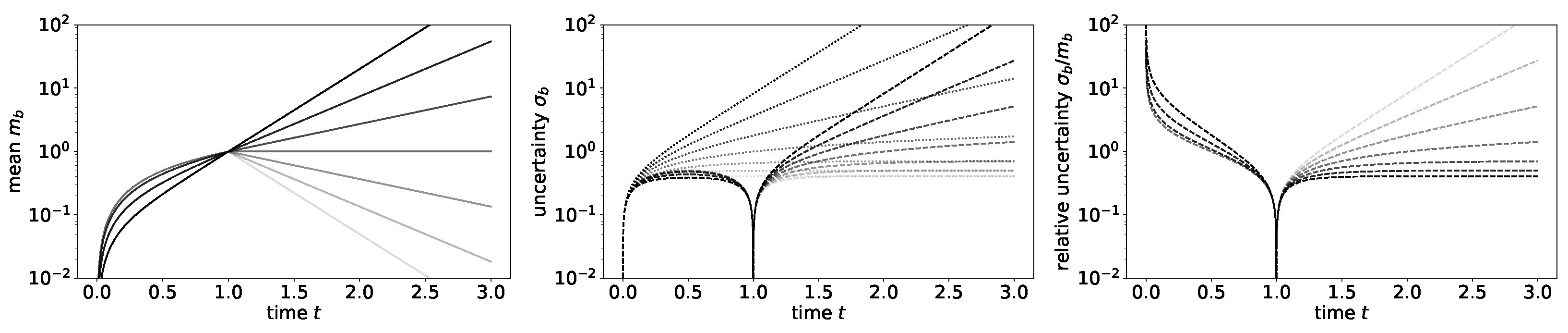
Figure 1 shows the prior and posterior mean and uncertainty for three different Lyapunov exponents ${\lambda }_b$ and a perfect measurement at $t_{\mathrm{o}}$. As we can see from Equation (20), the correlation between different modes $a\ne a^{\prime }$ vanishes, and therefore, any mode $a\ne b$ behaves like a prior mode shown in gray in Figure 1. Moreover, the propagator for the measured mode b is in general non-zero, but we can show that it vanishes for times, which are separated by the measurement, i.e., $D_{(b,t)(b,t^{\prime })}=0$ for $t<t_o<t^{\prime }$. In other words, the measurement introduces a Markov blanket. This Markov blanket separates the periods before and after the measurement from each other.

The impact of the Lyapunov exponents on the predictability of the system is clearly visible in Figure 1. The illustration shows that Lyapunov exponents which are greater than one lead to diverging uncertainties. In other words, chaos makes the inference more difficult on an absolute scale.

In Figure 2, we can see that the uncertainty grows faster for a larger Lyapunov exponent. Moreover, the relative uncertainty grows slower with increasing Lyapunov exponents, which mirrors the memory effect of a chaotic system. Thus, small initial disturbances can be remembered for long times.

In the case of nonlinear dynamics, the posterior knowledge becomes non-Gaussian, or in other words, the theory becomes interactive, i.e., it does not only incorporate the propagator and the source term but also interaction terms between more than two fields. At first, we will consider the case ${\lambda }_b=0$ and extend it to the next higher order in ${ϵ}_b=b^{†}ϵ(·,t)$,

$$\begin{array}{c}\hfill {\partial }_t{ϵ}_b=\frac{1}{2}{\mu }_b{ϵ}_b^2+\xi +\mathcal{O}({ϵ}_b^3)\to \tilde{G}[{ϵ}_b]={\partial }_t{ϵ}_b-\frac{1}{2}{\mu }_b{ϵ}_b^2.\end{array}$$

(21)

This leads to an information Hamiltonian that contains a free and an interaction part, $\mathcal{H}(d,ϵ,\chi ,\overline{\chi })={\mathcal{H}}_{\mathrm{free}}(d,ϵ,\chi ,\overline{\chi })+{\mathcal{H}}_{\mathrm{int}}(d,ϵ,\chi ,\overline{\chi })$,

$$\begin{array}{cc}\hfill {\mathcal{H}}_{\mathrm{free}}(d,\phi ,\chi ,\overline{\chi })& =\frac{1}{2}{\epsilon }_b^{†}{\partial }_t^{†}{\partial }_t{\epsilon }_b+{\overline{\chi }}^{†}{\partial }_t\chi +\mathcal{H}(d|\phi )+\mathcal{H}({\phi }_0)\hfill \\ \hfill {\mathcal{H}}_{\mathrm{int}}(d,\phi ,\chi ,\overline{\chi })& =-{\mu }_b{\left[{\epsilon }_b^2\right]}^{†}{\partial }_t{\epsilon }_b+\frac{{\mu }_b^2}{8}{\left[{\epsilon }_b^2\right]}^{†}\left[{\epsilon }_b^2\right]-{\mu }_b{\overline{\chi }}^{†}\left({\epsilon }_b\chi \right).\hfill \end{array}$$

The free information Hamiltonian ${\mathcal{H}}_{\mathrm{free}}(d,ϵ,\chi ,\overline{\chi })$ defines the Wiener process field inference problem we addressed before and has the classical field as well as the bosonic and fermionic propagators and interactions between the fields for $t<t_o$. It can be shown that all first-order diagrams with bosonic three-vertex are zero for ${\lambda }_b=0$ [18]. Thus, the posterior mean and uncertainty dispersion for $0\le t,t^{\prime }\le t_{\mathrm{o}}$ only contain corrections due to the fermion loop,

Now, we consider the case ${\lambda }_b\ne 0$, i.e., $\tilde{G}[{ϵ}_b]={\partial }_t{ϵ}_b-{\lambda }_b{ϵ}_b-\frac{1}{2}{\mu }_b{ϵ}_b^2$, such that

$$\begin{array}{cc}\hfill {\mathcal{H}}_{\mathrm{free}}(d,ϵ,\chi ,\overline{\chi })& =\frac{1}{2}{ϵ}_b^{†}\left[{({\partial }_t-{\lambda }_b)}^{†}({\partial }_t-{\lambda }_b)\right]{ϵ}_b+{\overline{\chi }}^{†}({\partial }_t-{\lambda }_b)\chi +\mathcal{H}(d|\phi )+\mathcal{H}({\phi }_0)\hfill \end{array}$$

(22)

$$\begin{array}{cc}\hfill {\mathcal{H}}_{\mathrm{int}}(d,ϵ,\chi ,\overline{\chi })& =-{\mu }_b{[{ϵ}_b^2]}^{†}({\partial }_t-{\lambda }_b){ϵ}_b+\frac{{\mu }_b^2}{8}{[{ϵ}_b^2]}^{†}[{ϵ}_b^2]-{\mu }_b{\overline{\chi }}^{†}({ϵ}_b\chi )\hfill \end{array}$$

(23)

The only changed vertex for this information Hamiltonian is the bosonic three-vertex, which does not vanish for ${\lambda }_b\ne 0$, leading to the following Feynman diagram representation of the posterior mean and uncertainty:

In any case, we can see that the fermionic loop correction appears independently of the eigenvalue of the measured mode ${\lambda }_b$ in the nonlinear case. Thus, taking into account the functional determinant, represented by the fermionic fields here, is important to arrive at the correct posterior values. The posterior values are calculated with the computer algebra system SymPy [23] and represented in Figure 3.

Note that the a priori mean and uncertainty dispersion are both infinite for any time $t>0$, as without the measurement, trajectories reaching positive infinity within finite times are not excluded from the ensemble of permitted possibilities. For times $t\in [0,t_{\mathrm{o}}]$, the posterior mean should stay finite as well as its uncertainty. The reason is that any diverging trajectory in this region is excluded by the measurement, as the dynamics do not allow trajectories to return from infinity as this would require an infinite excitation. The figure shows that in all displayed cases (${\lambda }_b\in \{-1,0,1\}$), the posterior trajectories avoid to get close to easily diverging regimes, and the more the dynamics is unstable, for larger values in ${\lambda }_b$, the more they avoid such regimes. Interestingly though, the posterior uncertainty of unstable systems with ${\lambda }_b>0$ in the period before the measurement is reduced in comparison with the posterior uncertainty of the stable system. In the end, this is in accordance with the statement that chaotic systems are harder to predict, as for chaotic systems the trajectories diverge, and thus, the variety of trajectories that pass through the initial and the measurement condition is smaller. Thus, for a chaotic system, the measurement provides more information on the period before the measurement but less for the period after the measurement.

6. Conclusions

Two of the challenges in DFI are the incorporation of the delta function and the Jacobian, which appear in the path integral over all possible solutions, in the inference. Here, advanced DFI schemes were developed, which introduce bosonic and fermionic auxiliary fields to circumvent the inference of the Jacobian. Using the introduced fields in perturbative calculations such as Feynman diagrams, might allow to develop DFI schemes in future research that can tackle the difficulties of inference in nonlinear systems. We showed that in the case of white Gaussian noise and no measurement constraint, the dynamical system in the language of DFI has a supersymmetry. For chaotic systems, mirrored by positive Lyapunov exponents, this supersymmetry is broken spontaneously leading to a lower predictability of the system. In order to illustrate the impact of chaos on the inference in linear and nonlinear systems, we considered two simplified scenarios, such that the inference problem becomes a one-dimensional problem for the measured mode. It turns out that the fermionic contributions for any eigenvalue of the measured mode are key to obtain the correct posterior mean. From the considered examples, we saw that as expected the prediction of a system’s absolute evolution from measurements is harder for a chaotic system. However, the relative uncertainty grows slower in a chaotic system, mirroring the memory effect of chaotic systems. Finally, predicting a nonlinear chaotic system gets even harder than for linear ones, but the information obtained from a measurement is enhanced, as more a priori possible trajectories are excluded by measurement in a chaotic system due to its larger sensitivity to perturbations. For future research, the analysis of more complex systems including the insights from STS can be interesting. For those, the inclusion of the fermionic corrections, as seen from the simplified scenarios, are likely to be essential to obtain the correct solution.

References

1. Krülls, W.; Achterberg, A. Computation of cosmic-ray acceleration by Ito’s stochastic differential equations. Astron. Astrophys. 1994, 286, 314–327. [Google Scholar]
2. Allen, L.J. An Introduction to Stochastic Processes with Applications to Biology; CRC Press: Boca Raton, FL, USA, 2010. [Google Scholar]
3. Gardiner, C.W. Handbook of Stochastic Methods; Springer: Berlin, Germany, 1985; Volume 3. [Google Scholar]
4. Mao, X. Stochastic Differential Equations and Applications; Elsevier: Amsterdam, The Netherlands, 2007. [Google Scholar]
5. Black, F.; Scholes, M. The pricing of options and corporate liabilities. In World Scientific Reference on Contingent Claims Analysis in Corporate Finance: Volume 1: Foundations of CCA and Equity Valuation; World Scientific: Singapore, 2019; pp. 3–21. [Google Scholar]
6. Galenko, P.; Kharchenko, D.; Lysenko, I. Stochastic generalization for a hyperbolic model of spinodal decomposition. Phys. A Stat. Mech. Its Appl. 2010, 389, 3443–3455. [Google Scholar] [CrossRef]
7. Uhlenbeck, G.E.; Ornstein, L.S. On the theory of the Brownian motion. Phys. Rev. 1930, 36, 823. [Google Scholar] [CrossRef]
8. Ovchinnikov, I.V. Topological field theory of dynamical systems. Chaos Solitons Fractals 2012, 22, 033134. [Google Scholar] [CrossRef] [PubMed] [Green Version]
9. Ovchinnikov, I.V. Introduction to Supersymmetric Theory of Stochastics. Entropy 2016, 18, 108. [Google Scholar] [CrossRef] [Green Version]
10. Ovchinnikov, I.V.; Schwartz, R.N.; Wang, K.L. Topological supersymmetry breaking: Definition and stochastic generalization of chaos and the limit of applicability of statistics. Mod. Phys. Lett. B 2016, 30, 1650086. [Google Scholar] [CrossRef] [Green Version]
11. Ovchinnikov, I.V.; Di Ventra, M. Chaos or Order? Mod. Phys. Lett. B 2019, 33, 1950287. [Google Scholar] [CrossRef]
12. Box, G.E.; Tiao, G.C. Bayesian Inference in Statistical Analysis; John Wiley & Sons: Hoboken, NJ, USA, 2011; Volume 40. [Google Scholar]
13. Jaynes, E.T. Probability Theory: The Logic of Science; Cambridge University Press: Cambridge, UK, 2003. [Google Scholar]
14. Doering, C.R. A stochastic partial differential equation with multiplicative noise. Phys. Lett. A 1987, 122, 133–139. [Google Scholar] [CrossRef]
15. Roberts, A.J. A step towards holistic discretisation of stochastic partial differential equations. ANZIAM J. 2003, 45, 1–15. [Google Scholar] [CrossRef] [Green Version]
16. Mukhanov, V.; Winitzki, S. Introduction to Quantum Effects in Gravity; Cambridge University Press: Cambridge, UK, 2007. [Google Scholar]
17. Enßlin, T.A. Information Theory for Fields. Ann. Phys. 2019, 531, 1800127. [Google Scholar] [CrossRef] [Green Version]
18. Westerkamp, M.; Ovchinnikov, I.; Frank, P.; Enßlin, T. Dynamical Field Inference and Supersymmetry. Entropy 2021, 23, 1652. [Google Scholar] [CrossRef] [PubMed]
19. Das, A. Field Theory: A Path Integral Approach, 2nd ed.; World Scientific Lecture Notes in Physics; World Scientific: Singapore, 2006. [Google Scholar]
20. Münster, G. Quantentheorie, 2nd ed.; De Gruyter: Berlin, Germany, 2010. [Google Scholar]
21. Bartelmann, M.; Feuerbacher, B.; Krüger, T.; Lüst, D.; Rebhan, A.; Wipf, A. Theoretische Physik; Springer Spektrum: Heidelberg, Germany, 2015. [Google Scholar]
22. Wiener, N. Generalized harmonic analysis. Acta Math. 1930, 55, 117–258. [Google Scholar] [CrossRef]
23. Meurer, A.; Smith, C.P.; Paprocki, M.; Čertík, O.; Kirpichev, S.B.; Rocklin, M.; Kumar, A.; Ivanov, S.; Moore, J.K.; Singh, S.; et al. SymPy: Symbolic computing in Python. PeerJ Comput. Sci. 2017, 3, e103. [Google Scholar] [CrossRef]
Figure 1. Illustration of the knowledge on a measured system mode b. A priori (gray) and a posteriori (magenta) field mean (lines) and one sigma uncertainty (shaded) for an Ornstein–Uhlenbeck process (left, λ b = 1 ) , a Wiener process (middle, λ b = 0 ) , and a chaotic process (right, λ b = 1 ) of a system eigenmode b after one perfect measurement at t o = 1 .
Psf 05 00027 g001
Figure 2. Illustration of the mean, uncertainty of the prior and posterior, as well as the relative posterior uncertainty on a measured system mode b on logarithmic scale for a set of Lyapunov exponents λ b = 3 , 2 , 1 , 0, 1, 2, and 3, as displayed in colors ranging from light to dark gray in this order (i.e., strongest chaos is shown in black). Left: Posterior mean. Middle: Uncertainty of prior (dotted) and posterior (dashed). Right: Relative posterior uncertainty.
Psf 05 00027 g002
Figure 3. Illustration of the knowledge on a measured system mode b like in Figure 1 for a nonlinear system within the period t [ 0 , 1 ] with first-order bosonic and fermionic perturbation corrections for μ b = 0.3 in green and without such nonlinear corrections in magenta, and with only bosonic corrections in blue (dotted, displayed without uncertainty). The three panels display the cases λ b = 1 (left), λ b = 0 (middle), and λ b = 1 (right).
Psf 05 00027 g003
Publisher’s Note: MDPI stays neutral with regard to jurisdictional claims in published maps and institutional affiliations.