
Geometric Learning of Hidden Markov Models via a Method of Moments Algorithm †


Abstract
:1. Introduction
1.1. Hidden Markov Models with Manifold-Valued Observations
1.2. Contributions and Paper Outline
1.3. Notation
2. Hidden Markov Models on Manifolds
3. Method of Moments Algorithms for Geometric Learning of Hidden Markov Models
3.1. Method of Moments for HMMs
- Solveand set .
- For , solveand set .
3.2. Geometric Learning of HMMs Using Method of Moments
- Solveand set .
- For , solveand set .
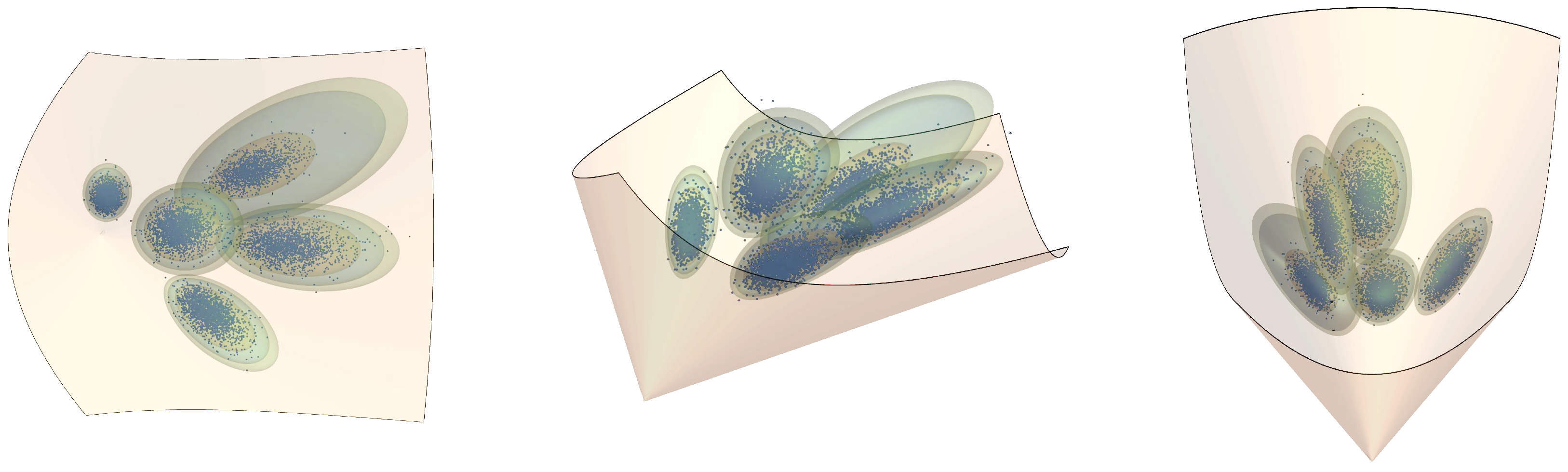
4. Simulations
4.1. Example 1: Observations in Hyperbolic Space
4.2. Example 2: Observations in the Manifold of SPD Matrices with Hidden States
5. Conclusions
Author Contributions
Funding
Institutional Review Board Statement
Informed Consent Statement
Data Availability Statement
Conflicts of Interest
References
- Krishnamurthy, V. Partially Observed Markov Decision Processes: From Filtering to Controlled Sensing; Cambridge University Press: Cambridge, UK, 2016. [Google Scholar] [CrossRef]
- Durbin, R.; Eddy, S.R.; Krogh, A.; Mitchison, G. Biological Sequence Analysis: Probabilistic Models of Proteins and Nucleic Acids; Cambridge University Press: Cambridge, UK, 1998. [Google Scholar] [CrossRef]
- Vidyasagar, M. Hidden Markov Processes: Theory and Applications to Biology; Princeton University Press: Princeton, NJ, USA, 2014. [Google Scholar]
- Cappé, O.; Moulines, E.; Rydén, T. Inference in hidden Markov models; Springer Science & Business Media: Berlin/Heidelberg, Germany, 2005. [Google Scholar]
- Rabiner, L. A tutorial on hidden Markov models and selected applications in speech recognition. Proc. IEEE 1989, 77, 257–286. [Google Scholar] [CrossRef] [Green Version]
- Gales, M.; Young, S. The application of hidden Markov models in speech recognition. Found. Trends Signal Process. 2008, 1, 195–304. [Google Scholar] [CrossRef]
- Mamon, R.S.; Elliott, R.J. Hidden Markov Models in Finance; Springer: Berlin/Heidelberg, Germany, 2007. [Google Scholar]
- Chang, J.T. Full reconstruction of Markov models on evolutionary trees: Identifiability and consistency. Math. Biosci. 1996, 137, 51–73. [Google Scholar] [CrossRef]
- Mossel, E.; Roch, S. Learning nonsingular phylogenies and hidden Markov models. Ann. Appl. Probab. 2006, 16, 583–614. [Google Scholar] [CrossRef] [Green Version]
- Hsu, D.; Kakade, S.M.; Zhang, T. A spectral algorithm for learning Hidden Markov Models. J. Comput. Syst. Sci. 2012, 78, 1460–1480. [Google Scholar] [CrossRef] [Green Version]
- Anandkumar, A.; Hsu, D.; Kakade, S.M. A Method of Moments for Mixture Models and Hidden Markov Models. In Proceedings of Machine Learning Research, Proceedings of the 25th Annual Conference on Learning Theory; Mannor, S., Srebro, N., Williamson, R.C., Eds.; PMLR: Edinburgh, UK, 2012; Volume 23, pp. 33.1–33.34. [Google Scholar]
- Kontorovich, A.; Nadler, B.; Weiss, R. On Learning Parametric-Output HMMs. In Proceedings of the 30th International Conference on International Conference on Machine Learning, ICML’13, Atlanta, GA, USA, 16–21 June 2013; JMLR.org. Volume 28, pp. III–702–III–710. [Google Scholar]
- Mattila, R.; Rojas, C.R.; Krishnamurthy, V.; Wahlberg, B. Asymptotically Efficient Identification of Known-Sensor Hidden Markov Models. IEEE Signal Process. Lett. 2017, 24, 1813–1817. [Google Scholar] [CrossRef]
- Huang, K.; Fu, X.; Sidiropoulos, N. Learning Hidden Markov Models from Pairwise Co-occurrences with Application to Topic Modeling. In Proceedings of Machine Learning Research, Proceedings of the 35th International Conference on Machine Learning; Dy, J., Krause, A., Eds.; PMLR: Edinburgh, UK, 2018; Volume 80, pp. 2068–2077. [Google Scholar]
- Mattila, R.; Rojas, C.; Moulines, E.; Krishnamurthy, V.; Wahlberg, B. Fast and Consistent Learning of Hidden Markov Models by Incorporating Non-Consecutive Correlations. In Proceedings of Machine Learning Research, Proceedings of the 37th International Conference on Machine Learning; Daumé, H.D., III, Singh, A., Eds.; PMLR: Edinburgh, UK, 2020; Volume 119, pp. 6785–6796. [Google Scholar]
- Mattila, R. Hidden Markov models: Identification, inverse filtering and applications. Ph.D. Thesis, KTH Royal Institute of Technology, Stockholm, Sweden, 2020. [Google Scholar]
- Absil, P.A.; Mahony, R.; Sepulchre, R. Optimization Algorithms on Matrix Manifolds; Princeton University Press: Princeton, NJ, USA, 2009. [Google Scholar] [CrossRef] [Green Version]
- Barachant, A.; Bonnet, S.; Congedo, M.; Jutten, C. Multiclass Brain–Computer Interface Classification by Riemannian Geometry. IEEE Trans. Biomed. Eng. 2012, 59, 920–928. [Google Scholar] [CrossRef] [PubMed]
- Boumal, N.; Mishra, B.; Absil, P.A.; Sepulchre, R. Manopt, a Matlab Toolbox for Optimization on Manifolds. J. Mach. Learn. Res. 2014, 15, 1455–1459. [Google Scholar]
- Pennec, X.; Sommer, S.; Fletcher, T. Riemannian Geometric Statistics in Medical Image Analysis; Academic Press: Cambridge, MA, USA, 2020. [Google Scholar]
- Miolane, N.; Guigui, N.; Brigant, A.L.; Mathe, J.; Hou, B.; Thanwerdas, Y.; Heyder, S.; Peltre, O.; Koep, N.; Zaatiti, H.; et al. Geomstats: A Python Package for Riemannian Geometry in Machine Learning. J. Mach. Learn. Res. 2020, 21, 1–9. [Google Scholar]
- Mostajeran, C.; Grussler, C.; Sepulchre, R. Geometric Matrix Midranges. SIAM J. Matrix Anal. Appl. 2020, 41, 1347–1368. [Google Scholar] [CrossRef]
- Van Goffrier, G.W.; Mostajeran, C.; Sepulchre, R. Inductive Geometric Matrix Midranges. IFAC-PapersOnLine 2021, 54, 584–589. [Google Scholar] [CrossRef]
- Said, S.; Le Bihan, N.; Manton, J. Hidden Markov chains and fields with observations in Riemannian manifolds. IFAC-PapersOnLine 2021, 54, 719–724. [Google Scholar] [CrossRef]
- Tupker, Q.; Said, S.; Mostajeran, C. Online Learning of Riemannian Hidden Markov Models in Homogeneous Hadamard Spaces. In Geometric Science of Information; Nielsen, F., Barbaresco, F., Eds.; Springer International Publishing: Cham, Switzerland, 2021; pp. 37–44. [Google Scholar]
- Said, S.; Bombrun, L.; Berthoumieu, Y.; Manton, J.H. Riemannian Gaussian Distributions on the Space of Symmetric Positive Definite Matrices. IEEE Trans. Inf. Theory 2017, 63, 2153–2170. [Google Scholar] [CrossRef] [Green Version]
- Said, S.; Hajri, H.; Bombrun, L.; Vemuri, B.C. Gaussian Distributions on Riemannian Symmetric Spaces: Statistical Learning With Structured Covariance Matrices. IEEE Trans. Inf. Theory 2018, 64, 752–772. [Google Scholar] [CrossRef]
- Said, S.; Mostajeran, C.; Heuveline, S. Gaussian distributions on Riemannian symmetric spaces of nonpositive curvature. In Handbook of Statistics; Elsevier: Amsterdam, The Netherlands, 2022. [Google Scholar] [CrossRef]
- Heuveline, S.; Said, S.; Mostajeran, C. Gaussian Distributions on Riemannian Symmetric Spaces in the Large N Limit. In Geometric Science of Information; Nielsen, F., Barbaresco, F., Eds.; Springer International Publishing: Cham, Switzerland, 2021; pp. 20–28. [Google Scholar]
- Santilli, L.; Tierz, M. Riemannian Gaussian distributions, random matrix ensembles and diffusion kernels. Nucl. Phys. B 2021, 973, 115582. [Google Scholar] [CrossRef]
- Said, S.; Heuveline, S.; Mostajeran, C. Riemannian statistics meets random matrix theory: Towards learning from high-dimensional covariance matrices. IEEE Trans. Inf. Theory 2022. submitted for publication. [Google Scholar] [CrossRef]
- Zanini, P.; Said, S.; Cavalcante, C.C.; Berthoumieu, Y. Stochastic EM algorithm for mixture estimation on manifolds. In Proceedings of the 2017 IEEE 7th International Workshop on Computational Advances in Multi-Sensor Adaptive Processing (CAMSAP), Curacao, The Netherlands, 10–13 December 2017; pp. 1–5. [Google Scholar] [CrossRef]
- Zanini, P.; Said, S.; Berthoumieu, Y.; Congedo, M.; Jutten, C. Riemannian Online Algorithms for Estimating Mixture Model Parameters. In Geometric Science of Information (GSI 2017); Springer: Berlin/Heidelberg, Germany, 2017. [Google Scholar] [CrossRef]
- Nickel, M.; Kiela, D. Poincaré Embeddings for Learning Hierarchical Representations. In Advances in Neural Information Processing Systems; Guyon, I., Luxburg, U.V., Bengio, S., Wallach, H., Fergus, R., Vishwanathan, S., Garnett, R., Eds.; Curran Associates, Inc.: Red Hook, NY, USA, 2017; Volume 30. [Google Scholar]
- Said, S.; Bombrun, L.; Berthoumieu, Y. New Riemannian Priors on the Univariate Normal Model. Entropy 2014, 16, 4015–4031. [Google Scholar] [CrossRef]


| EM Algorithm from [24] | Online Algorithm from [25] | Our proposed algorithm with (a) , (b) , (c) | |
|---|---|---|---|
| Mean error, | 0.88 | 0.97 | 0.69 |
| Dispersion error, | 0.42 | 0.37 | 0.34 |
| Transition matrix error, | 0.35 | 0.30 | (a) 0.42, (b) 0.26, (c) 0.21 |
| Average runtime | ∼1 h | ∼190 s | ∼20 s |
Publisher’s Note: MDPI stays neutral with regard to jurisdictional claims in published maps and institutional affiliations. |
© 2022 by the authors. Licensee MDPI, Basel, Switzerland. This article is an open access article distributed under the terms and conditions of the Creative Commons Attribution (CC BY) license (https://creativecommons.org/licenses/by/4.0/).
Share and Cite
Chen, B.; Mostajeran, C.; Said, S. Geometric Learning of Hidden Markov Models via a Method of Moments Algorithm. Phys. Sci. Forum 2022, 5, 10. https://doi.org/10.3390/psf2022005010
Chen B, Mostajeran C, Said S. Geometric Learning of Hidden Markov Models via a Method of Moments Algorithm. Physical Sciences Forum. 2022; 5(1):10. https://doi.org/10.3390/psf2022005010
Chicago/Turabian StyleChen, Berlin, Cyrus Mostajeran, and Salem Said. 2022. "Geometric Learning of Hidden Markov Models via a Method of Moments Algorithm" Physical Sciences Forum 5, no. 1: 10. https://doi.org/10.3390/psf2022005010