
Electron Born Self-Energy Model for Dark Energy †


Department of Physics, 116 Cardwell Hall, Kansas State University, Manhattan, KS 66506-2601, USA
†
Presented at the 1st Electronic Conference on Universe, 22–28 February 2021; Available online: https://ecu2021.sciforum.net/.
Phys. Sci. Forum 2021, 2(1), 9; https://doi.org/10.3390/ECU2021-09300
Published: 22 February 2021
(This article belongs to the Proceedings of The 1st Electronic Conference on Universe)
Abstract
:Dark Energy, a form of repulsive gravity, is causing an accelerated expansion of the Universe. Recent astrophysical measurements have confirmed this accelerated expansion where the ΛCDM model provides a quantitative description of this expansion rate. As is well known there are a number of free parameters of unknown origin in the ΛCDM model. In particular, the cosmological constant Λ (or Dark Energy (DE)) forms one of these free parameters. In this contribution we describe a recent model that attributes DE to the Born self-energy contained within the electric field which surrounds a finite-sized electron within the WHIM (Warm-Hot Intergalactic Medium). Upon using readily available literature values for the intergalactic (IG) baryon density, IG hydrogen ionization fraction, the best estimate for the electron radius, as well as, Hubble parameter data many properties associated with DE can be quantitatively explained. In particular, our model provides an explanation for (i) the magnitude of DE today, (ii) the DE to ordinary matter mass ratio today, (iii) has an equation of state of w = −1, as expected for DE, and (iv) exhibits a deceleration-acceleration transition at a redshift of z~0.8 in agreement with Hubble parameter observations. (v) Finally, the model provides a viable candidate for Dark Matter; the CDM in the ΛCDM model.Further details regarding this DE model can be found in Astrophys. Space Sci 2020, 365, 64.
1. Introduction
The cosmological ΛCDM model provides a remarkable description of many diverse astrophysical phenomena including the cosmic microwave background (CMB) anisotropy [1], the relative proportions of the light elements [1], and the cosmic expansion rate as measured from galactic supernova explosions in the distant past [2,3]. Despite the tremendous success of the ΛCDM model there are a number of adjustable parameters in this model whose physical origin is an enduring mystery. Specifically, the cosmological constant Λ or, more generically, Dark Energy is thought to arise from the Casimir effect or quantum fluctuations in intergalactic space, however, the energy density estimated for this effect (where is the Planck mass, is the Planck length, and is the speed of light) is a factor of larger than astrophysical measurements [4]. Thus, in the ΛCDM model the magnitude of Dark Energy and corresponding properties attributed to Dark Energy are not understood and currently there is no plausible explanation for these properties. In a similar manner the origin of Cold Dark Matter, the CDM in the ΛCDM model, is of unknown origin. Thus, this quantity is also an adjustable parameter.
The purpose of this contribution is to describe a recently published theory [5] which quantitatively explains Dark Energy and attributes this repulsive gravity to the Born self-energy contained within the electric field which surrounds high temperature () free electrons in the Warm-Hot-Intergalactic-Medium (WHIM) [6,7]. This theory also includes a phenomenon which would naturally give rise to Dark Matter, specifically, the Born self-energy associated with cold electrons in intergalactic space.
2. Results
If the CMB, at a redshift , is fitted using the ΛCDM model and this model is extrapolated to the current epoch (i.e., to today at ) then the ΛCDM parameters listed in Table 1 arise from this fitting. Similar values for the mass fractions and energy densities, given in Table 1, also arise if the ΛCDM model is fitting to other types of astrophysical data [1] (p. 19).
Any successful theory for DE, therefore, would need to account for the following four facts:
- The magnitude of the DE listed in Table 1, specifically,where subscript is to denote that this quantity arises from the Planck collaboration.
- The DE to Ordinary Matter (OM) mass ratio given in Table 1. Specifically,
- The equation of state for DE is expected to be [9]where is the pressure. The in Equation (3) implies that DE is a form of repulsive gravity which causes the Universe to expand at an accelerating rate. This is most readily seen using the Friedmann acceleration equation [10]where is the scale factor, is the acceleration of the scale factor, and is Newton’s gravitational constant. The second line in Equation (4) arises from Equation (3) with the assumption that DE is the dominant contribution to the scale factor acceleration. Normally gravity is thought of as an attractive force when applied to ordinary matter and, under such circumstances, the expansion of the Universe should be decelerating (). This leads to the fourth observation that a theory for DE must be able to account for.
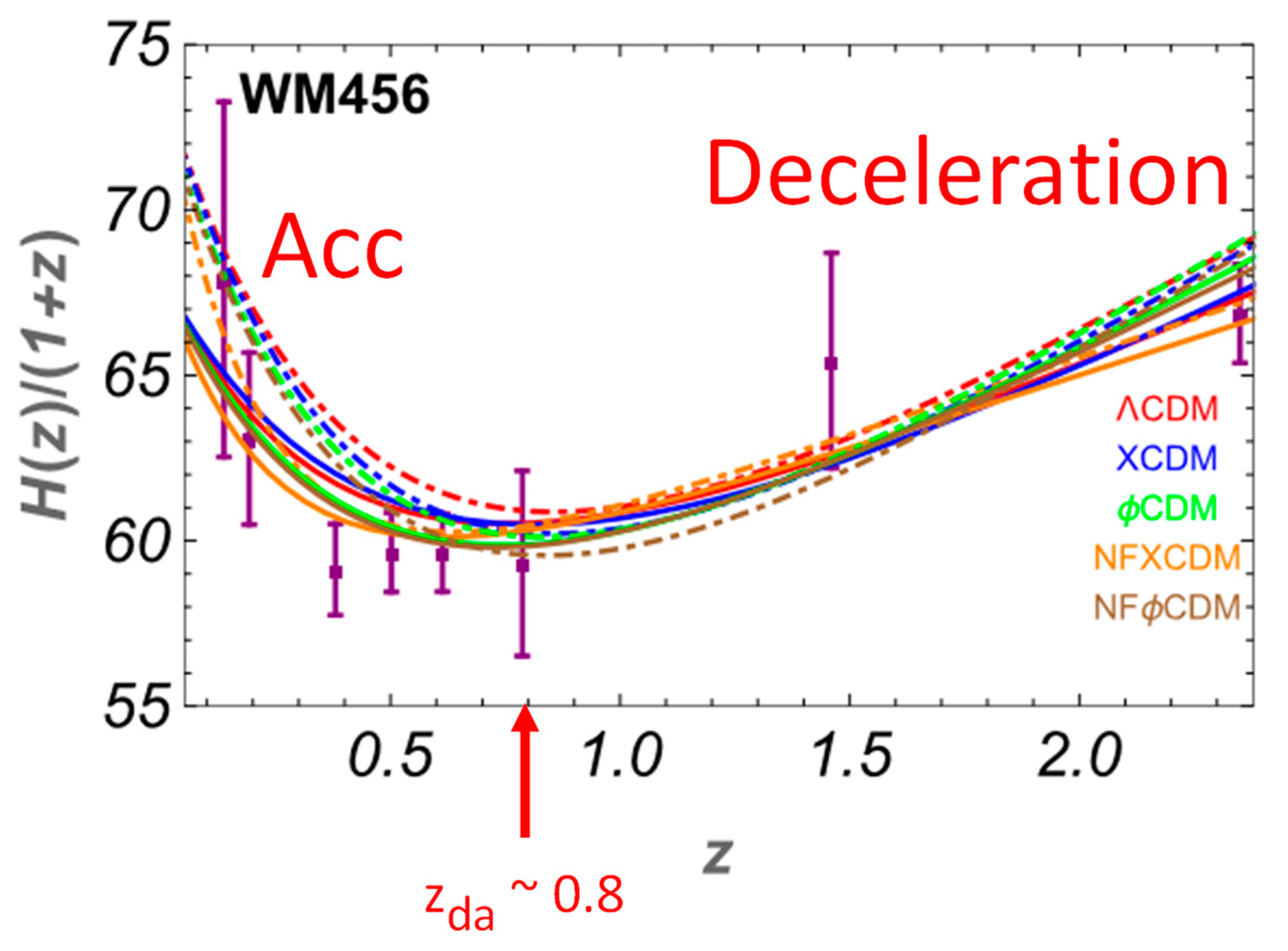
- There must be a transition from a decelerating to an accelerating Universe. This transition is readily observed in Figure 1 which consists of “WM456” binned data taken from [11]. In this figure , the velocity scale factor, which arises from Hubble’s law, , together with . When the ΛCDM model is fitted to such binned data a deceleration-acceleration transition is found at a redshift of [11]
3. Discussion
3.1. Born Self-Energy for the Electron
In 2013 the author was listening to an invited talk given by Professor Alan Guth on “Inflationary Cosmology: Is our Universe part of a multiverse?” at Kansas State University. In this talk Professor Guth mentioned that the cosmological constant was thought to arise from the Casimir effect, due to vacuum fluctuations in empty space, except that such a calculation produced an answer which was a factor of times larger than astrophysical measurements. This statement intrigued the author who had previously published numerous papers on the surface Casimir effect within thin films for real systems [12,13] and had recently determined how to calculate the Casimir self-energy for a dielectric spherical ball (with the objective to see if the Casimir self-energy could explain the monodispersity of nanoparticles). On a very crude level a hydrogen atom in intergalactic space is a dielectric spherical ball. For dielectric systems the dielectric constant approaches one at ultra violet frequencies, hence, this provides a physical cut-off for the Casimir effect. Could this uv cut-off to the Casimir effect provide an explanation for the factor of ? This was the thought process that lead the author to investigate the energy densities arising from electric field contributions, for hydrogen and ionized hydrogen, in intergalactic space.
According to Table 1 intergalactic space consists of one hydrogen atom in a box of volume . This hydrogen atom is either ionized (into a proton and an electron) or un-ionized where the ionization (un-ionization) fraction is (). A hydrogen atom has a Casimir self-energy associated with it [14] (p. 103) given by
The proton and electron have a Born self-energy, due to the energy contained within the electric field which surrounds these particles [15] (pp. 8–12), [16] (p. 61), given by
where and are, respectively, the charge and radius of the particle. Therefore, according to this model, the total electric field energy density for intergalactic space is
In Equation (8) is dominated by the Born self-energy due to the electron because the electron radius, estimated from electron-positron collisions [17,18]
is so small. The ionization fraction,
arises from X-ray absorption measurements in intergalactic space [19]. The electric field energy density (Equation (8)) quantitatively agrees, within error bars, with the magnitude of the DE energy density given in Equation (1).
In this model the electron Born to Ordinary Matter mass ratio is given by
where () is the rest mass for the electron (proton). Equation (11) quantitatively agrees with Equation (2).
A standard method for calculating the pressure of a gas, contained within a box, is to examine the kinematics of molecules being reflected by the wall of this box [20]. Similarly, for the current situation, the pressure can be determined by examining an electron reflecting from a perfectly conducting wall. If an electron of charge is at a distance to the right of the wall, the correct electrostatic boundary conditions on the wall can be reproduced by considering an image charge with charge at a distance to the left of the wall [21] (p. 110). It is then possible to dispense with the wall and just consider the interaction of the charge with its image charge. Simple algebra, outlined in [5], demonstrates that the equation of state for this situation, which agrees with Equation (3) for DE.
The fourth and last point raised in Section 2 is “Can this DE model explain the deceleration-acceleration transition at a redshift of ?”. The first Friedmann equation is given by [10]
where, in our model, the cosmological constant is unnecessary () and the spatial curvature is zero while the energy density
In Equation (13) () is the energy density for Ordinary Matter (Dark Matter) while is the baryon number density given in Table 1. Equations (12) and (13) are readily rearranged to express the ionization fraction as a function of the Hubble parameter and redshift , specifically,
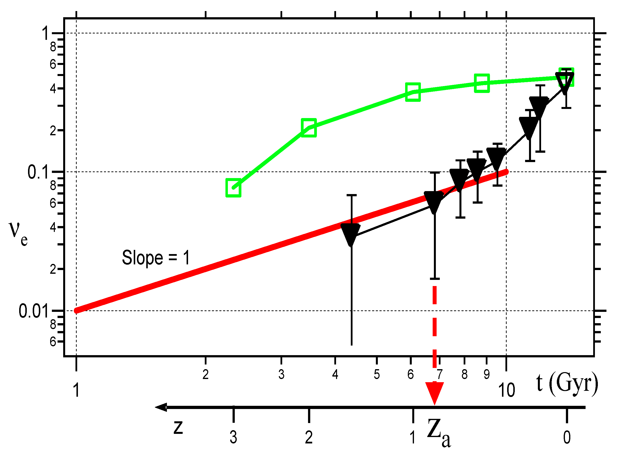
Equation (14) has been used to determine a log-log plot of the fractional ionization as a function of redshift or time (Figure 2, black inverted triangles) using the W456 Hubble parameter data [11] together with the Hubble constant from [22]. versus is the most illuminating. If we assume a time variation for the fractional ionization of
then the exponent determines whether the Universe is accelerating or decelerating. From Equations (12), (13), and (15)
which has solution
Thus, an accelerating Universe () implies that . In Figure 2 the solid red line corresponds to a slope of 1; therefore, a redshift of delineates the transition point between deceleration and acceleration for the W456 data (black inverted triangles) in approximate agreement with Equation (5). The time variation of arises from hydrogen gas, in low density voids in intergalactic space, falling into and becoming ionized by collisions with the high density filamentary network at temperatures of , namely, the WHIM. The variation in with time exhibited Figure 2 (black inverted triangles) is a prediction that arises from this theory; it would be useful if this prediction could be check via other astrophysical measurements. For example, perhaps the kinematic Sunyaev-Zel’dovich effect could provide a measure of the free electron distribution in intergalactic space [23]. (The green squares in Figure 2 represent determined in the WHIM from computer simulations [7] and are discussed in [5].)
Cold (free) electrons will also exist in intergalactic space, for example, left over from the re-ionization phase at redshifts of [24]. These cold electrons will also have an associated which would be evident via their gravitational interaction with other matter. These cold electrons could be the source for Dark Matter. If they are the sole source for Dark Matter then, in analogy with Equations (2) and (11), the DM ionization fraction would be determined by
where the second line of Equation (18) arises from the Ω values in Table 1. The total electron ionization fraction in intergalactic space would then be
where the first term on the right gives rise to DM while the second term on the right, , gives rise to DE when .
3.2. The Electron: A Revised View
The electron has played a key role in ascertaining and probing the quantum mechanical nature of matter. Quantum Electrodynamics (QED), which describes the interaction between electrons and photons, forms part of the Standard Model of Particle Physics. In QED the electron is assumed to be a point particle of zero radius (); unfortunately, this assumption leads to divergences in the mass and in the charge which must be renormalized away [25,26]. Upon renormalizing these divergences QED provides exquisite agreement between theory and experiment to many significant figures in, for example, the Lamb shift [27] and the electron magnetic moment [27,28]. The current theory amounts to a reorganization of the mass renormalized components of QED while leaving the other components of QED (used in the calculation of the Lamb shift and the electron magnetic moment) unchanged.
In QED mass renormalization corresponds to [25] (p. 164)
where the unmeasureable terms to the left of the arrow (which appear in the theory) are replaced by the measured electron rest mass, to the right of the arrow. In this equation is the Compton wavelength, is the bare mass (that occurs in the Dirac equation), while the ln term is the quantum mechanical self-energy due to virtual particles “dressing” the bare mass (i.e., corrections arising from an electron emitting and reabsorbing virtual photons, or other virtual particles, due to underlying quantum fluctuations) [27]. The positively divergent ln term is compensated by a negatively divergent bare mass so that the difference is given by the finite measured electron rest mass [29]. The Born self-energy is assumed to be subsumed within in QED and is therefore not explicitly considered. Namely, is assumed to be composed of both an inertial mass as well as an electromagnetic mass due to the electric field which surrounds the electron [30,31]. It was thought (in the 1950s) that there is no physical effect that could distinguish between and , hence, both terms were therefore combined together within [31] (p. 31). Both Dirac [29] and Feynman [32] expressed reservations about this renormalization process because the difference between two infinitely diverging terms is replaced by a finite quantity; however, renormalization now forms an accepted component of QED.
An issue with the renormalization process, as represented by Equation (20), is that the total energy is not conserved [15] (pp. 8–12). This is most readily apparent upon considering an electron-positron pair. On the point of annihilation the electron has energy but also, according to the current picture, a free electron also has energy . However, one must do work in separating the electron from the positron in order to create a free electron. Energy conservation therefore implies that a free electron must have a greater energy (due to the work done in this separation process) than an electron which is on the point of annihilation.
Our theory separates out the Born mass from and, as will become apparent below, restores energy conservation. It is illuminating to consider the total energy of a quasi-static electron-positron pair at a separation distance where all energy terms are explicitly considered
The last term on the right corresponds to the Coulomb attraction between the positron and electron. Upon annihilation (), with the emission of two photons to conserve both energy and momentum, the electric field terms in Equation (21) disappear and
Equation (22) reproduces the mass renormalization in Equation (20); thus, mass renormalization is required and is the result of energy conservation in the annihilation process . Equation (21) additionally allows one to determine the energy of a free electron, specifically,
and therefore , that appears in Equation (23), arises from the work done against the Coulomb interaction in separating the electron-positron pair (and is a necessary component in order that energy be conserved).
Ninham and Boström [33] have pointed out that the Casimir self-energy for the electron has been omitted from considerations in this theory. This term, which was first calculated by Boyer [34], takes the form
In order to leave QED unchanged and to retain energy conservation, must either be renormalized away or, alternatively, absorbed within the definition of in the considerations above.
In this theory the electron possesses two masses, the conventional rest mass , which arises from the coupling between the electron’s charge and applied (external) electric and magnetic fields, as described by the Lorentz equation
The electron has a second and much larger gravitational mass given by
where the Born mass is disconcertingly large,
which is times larger than and times larger than . In this theory it is the large magnitude for , as well as, the equation of state (Equation (3)) that gives rise to Dark Energy and a Dark Matter candidate. The gravitational mass arises because, in the Friedmann equation (Equation (12)), gravity couples to all energy sources. Note that if indeed is the origin for Dark Matter then this term would only be evident via its gravitational interaction and could not be measured directly via a Dark Matter search as, for example, does not enter into Equation (25).
4. Conclusions
This publication describes and expands upon a recently published model for Dark Energy [5]. In this model, DE is attributed to the Born self-energy contained within the electric field which surrounds a finite-sized free electron (of radius ) within the Warm-Hot Intergalactic Medium at temperatures of . The hydrogen ionization within WHIM varies with time or, correspondingly, redshift where or determined in this theory is depicted in Figure 2 (black inverted triangles). A transition from a decelerating to an accelerating Universe occurs at a transition redshift of . Upon combining the hydrogen ionization in the current epoch with and the known baryon number density then this model provides an explanation for both the magnitude of the DE energy density (Equations (1) and (8)), as well as, the DE to OM mass ratio (Equations (2) and (11)) today. This model also naturally gives rise to a Dark Matter candidate, namely, the Born self-energy associated with cold free electrons at temperatures in intergalactic space.
QED assume that the electron is a point particle of zero radius . This point particle assumption leads to divergences in the mass and in the charge that must be renormalized away. QED provides exquisite agreement with experimental measurements for both the Lamb shift and the electron magnetic moment, therefore, in our finite-sized electron model for DE it is necessary to ensure that QED remains unchanged. Our model and its relationship to QED is discussed in detail in Section 3.2 where it is argued that, by a suitable rearrangement of terms, both mass renormalization as well as arise naturally out of energy conservation considerations while leaving QED unchanged. This is an improvement on QED where mass renormalization is an ad hoc assumption.
Acknowledgments
The author has benefited from numerous discussions and comments from Professors Mathias Boström, Louis Crane, Barry Ninham, James Peebles, Bharat Ratra, Larry Weaver, as well as, anonymous referees.
Conflicts of Interest
The author declares no conflict of interest.
Abbreviations
The following abbreviations are used in this manuscript:
| CMB | Cosmic Microwave Background |
| DE | Dark Energy |
| DM | Dark Matter |
| OM | Ordinary Matter |
| QED | Quantum Electrodynamics |
| WHIM | Warm-Hot Intergalactic Medium |
References
- Peebles, P.J.E.; Page, L.A., Jr.; Partridge, R.B. Finding the Big Bang; Cambridge University Press: Cambridge, UK, 2009. [Google Scholar]
- Riess, A.G.; Filippenko, A.V.; Challis, P.; Clocchiatti, A.; Diercks, A.; Garnavich, P.M.; Gilliland, R.L.; Hogan, C.J.; Jha, S.; Kirshner, R.P.; et al. Observational evidence from supernovae for an accelerating Universe and a cosmological constant. Astron. J. 1998, 16, 1009. [Google Scholar] [CrossRef] [Green Version]
- Perlmutter, S.; Aldering, G.; Goldhaber, G.; Knop, R.A.; Nugent, P.; Castro, P.G.; Deustua, S.; Fabbro, S.; Goobar, A.; Groom, D.E.; et al. Measurements of Ω and Λ from 42 high-redshift supernovae. Astrophys. J. 1999, 517, 565. [Google Scholar] [CrossRef]
- Carroll, S.M. The cosmological constant. Living Rev. Relativ. 2001, 4, 1. [Google Scholar] [CrossRef] [PubMed] [Green Version]
- Law, B.M. Cosmological consequences of a classical finite-sized electron model. Astrophys. Space Sci. 2020, 365, 64. [Google Scholar] [CrossRef]
- Dave, R.; Cen, R.; Ostriker, J.P.; Bryan, G.L.; Hernquist, L.; Katz, N.; Weinberg, D.H.; Norman, M.L.; O’Shea, B. Baryons in the warm-hot intergalactic medium. Astrophys. J. 2001, 552, 473–483. [Google Scholar] [CrossRef] [Green Version]
- Cen, R.; Ostriker, J.P. Where are the baryons? II. Feedback effects. Astrophys. J. 2006, 650, 560–572. [Google Scholar] [CrossRef] [Green Version]
- PlanckCollaboration. Planck 2018 results. VI. Cosmological parameters. Astron. Astrophys. 2018, arXiv:1807.06209. [Google Scholar]
- Frieman, J.A.; Turner, M.S.; Huterer, D. Dark Energy and the Accelerating Universe. Annu. Rev. Astron. Astrophys. 2008, 46, 385–432. [Google Scholar] [CrossRef] [Green Version]
- Liddle, A.R.; Lyth, D.H. Cosmological Inflation and Large-Scale Structure; Cambridge University Press: Cambridge, UK, 2000. [Google Scholar]
- Farooq, O.; Madiyar, F.R.; Crandall, S.; Ratra, B. Hubble parameter measurement constraints on the redshift of the deceleration-acceleration transition, dynamical Dark Energy, and space curvature. Astrophys. J. 2017, 835, 1–11. [Google Scholar] [CrossRef] [Green Version]
- Law, B.M. Metastable wetting layers. Phys. Rev. E 1993, 48, 2760–2765. [Google Scholar] [CrossRef] [PubMed]
- Law, B.M. Nucleated wetting films: The late-time behavior. Phys. Rev. E 1994, 50, 2827–2833. [Google Scholar] [CrossRef]
- Mahanty, J.; Ninham, B.W. Dispersion Forces; Academic Press: London, UK, 1976. [Google Scholar]
- Feynman, R.P.; Leighton, R.; Sands, M. The Feynman Lectures on Physics; Addison-Wesley: Reading, MA, USA, 1964; Volume II. [Google Scholar]
- Israelachvili, J.N. Intermolecular and Surface Forces, 3rd ed.; Academic Press: London, UK, 2011. [Google Scholar]
- Bourilkov, D. Hint for axial-vector contact interactions in the data on e+e− →e+e−(γ) at center-of-mass energies 192–208 GeV. Phys. Rev. D 2001, 64, 071701R. [Google Scholar] [CrossRef] [Green Version]
- Gabrielse, G.; Hanneke, D.; Kinoshita, T.; Nio, M.; Odom, B. New determination of the fine structure constant from the electron g value and QED. Phys. Rev. Lett. 2006, 97, 030802. [Google Scholar] [CrossRef] [Green Version]
- Bykov, A.M.; Paerels, F.B.S.; Petrosian, V. Equilibration processes in the Warm-Hot Intergalactic Medium. Space Sci. Rev. 2008, 134, 141. [Google Scholar] [CrossRef] [Green Version]
- Reif, F. Fundamental of Statistical and Thermal Physics; Mc-Graw Hill: New York, NY, USA, 1965. [Google Scholar]
- Jackson, J.D. Classical Electrodynamics; John Wiley & Sons, Inc.: New York, NY, USA, 1962. [Google Scholar]
- Riess, A.G.; Macri, L.M.; Hoffmann, S.L.; Scolnic, D.; Casertano, S.; Filippenko, A.V.; Tucker, B.E.; Reid, M.J.; Jones, D.O.; Silverman, J.M.; et al. A 2.6% determination of the local value of the Hubble constant. Astrophys. J. 2016, 826, 1–31. [Google Scholar] [CrossRef]
- Hill, J.C.; Ferraro, S.; Battaglia, N.; Liu, J.; Spergel, D.N. Kinematic Sunyaev-Zel’dovich effect with projected fields: A novel probe of the baryon distribution with Planck, WMAP, and WISE data. Phys. Rev. Lett. 2016, 117, 051301. [Google Scholar] [CrossRef] [Green Version]
- Wise, J.H. Cosmic reionisation. Contemp. Phys. 2019, 60, 145–163. [Google Scholar] [CrossRef] [Green Version]
- Bjorken, J.D.; Drell, S.D. Relativistic Quantum Mechanics; McGraw-Hill: New York, NY, USA, 1964. [Google Scholar]
- Sakurai, J.J. Advanced Quantum Mechanics; Benjamin/Cummings: Menlo Park, CA, USA, 1967. [Google Scholar]
- Weisskopf, V.F. The development of field theory in the last 50 years. Phys. Today 1981, 34, 69–85. [Google Scholar] [CrossRef]
- Odom, B.; Hanneke, D.; D’Urso, B.; Gabrielse, G. New measurement of the electron magnetic moment using a one-electron quantum cyclotron. Phys. Rev. Lett. 2006, 97, 030801. [Google Scholar] [CrossRef] [Green Version]
- Dirac, P.A.M. The evolution of the physicist’s picture of nature. Sci. Am. 1963, 208, 45. [Google Scholar] [CrossRef]
- Bethe, H.A. The electromagnetic shift of energy levels. Phys. Rev. 1947, 72, 339–341. [Google Scholar] [CrossRef]
- Heitler, W. The Quantum Theory of Radiation, 3rd ed.; Dover: New York, NY, USA, 1984. [Google Scholar]
- Feynman, R.P. QED: The Strange Theory of Light and Matter; Princeton University Press: Princeton, NJ, USA, 1985. [Google Scholar]
- Ninham, B.W.; Australian National University, Canberra, Australia; Boström, M.; University of Oslo, Oslo, Norway. Personal communication, 2020.
- Boyer, T.H. Quantum electromagnetic zero-point energy of a conducting spherical shell and the Casimir model for a charged particle. Phys. Rev. 1968, 174, 1764. [Google Scholar] [CrossRef]
Figure 1.
Binned “WM456” Hubble parameter data plotted as versus (symbols). Various theoretical fits to this binned data (lines). Taken from [11]. © AAS. Reproduced with permission.
Figure 1.
Binned “WM456” Hubble parameter data plotted as versus (symbols). Various theoretical fits to this binned data (lines). Taken from [11]. © AAS. Reproduced with permission.

Figure 2.
Fractional ionization plotted on a log-log graph as a function of redshift and time . Black inverted triangles: calculated using Equation (14); green squares: from computer simulations [7]. Reprinted by permission from RightsLink: Springer Nature, Law, B. M., Astrophys Space Sci 365, 64, [COPYRIGHT] (2020).


Table 1.
Average composition of the Universe today.
| Mass Fraction Ω | Volume per Baryon (m3) | Energy Density Π (J/m3) | |
|---|---|---|---|
| Dark Energy | |||
| Dark Matter | |||
| Ordinary Matter (Intergalactic diffuse gas/plasma) |
Planck collaboration: ΛCDM model, from the last column in Table 2 in [8].
Publisher’s Note: MDPI stays neutral with regard to jurisdictional claims in published maps and institutional affiliations. |
© 2021 by the author. Licensee MDPI, Basel, Switzerland. This article is an open access article distributed under the terms and conditions of the Creative Commons Attribution (CC BY) license (https://creativecommons.org/licenses/by/4.0/).
Share and Cite
MDPI and ACS Style
Law, B.M. Electron Born Self-Energy Model for Dark Energy. Phys. Sci. Forum 2021, 2, 9. https://doi.org/10.3390/ECU2021-09300
AMA Style
Law BM. Electron Born Self-Energy Model for Dark Energy. Physical Sciences Forum. 2021; 2(1):9. https://doi.org/10.3390/ECU2021-09300
Chicago/Turabian StyleLaw, Bruce M. 2021. "Electron Born Self-Energy Model for Dark Energy" Physical Sciences Forum 2, no. 1: 9. https://doi.org/10.3390/ECU2021-09300