Gravitoelectromagnetism: L’art Pour L’art—Or a Subject for the Classroom ^†

Abstract

At school and university, gravity is taught essentially in the Newtonian way. Newtonian mechanics originated at a time when there were no fields, when energy did not exist as a physical quantity, and when one still had to be satisfied with the concept of actions at a distance. A theory without such shortcomings, Maxwell’s electromagnetism, came into being about 150 years later. It could have served as a model for a modern theory of gravitation. In fact, such a theory of gravitation, gravitoelectromagnetism, was proposed by Heaviside. However, it did not establish itself, because, first, many effects it describes are very, very small; second, it makes certain statements that seem unacceptable to some researchers; and third, shortly thereafter, general relativity was born, which removed the old deficiencies and seemed to make a classical field theory of gravity superfluous. We argue that the subject of gravitoelectromagnetism is a legitimate one for teaching at school and university even now. On the one hand, general relativity is impractical for many applications because the mathematical effort is high, and on the other hand, the theory of gravitoelectromagnetism by no means describes only tiny effects. Rather, it solves a problem that is deliberately ignored in the traditional teaching of Newtonian mechanics: to which system do we assign the so-called potential energy? Where is the “potential” energy located? We also encounter some peculiarities of gravitoelectromagnetism that are caused by the fact that compressive and tensile stresses within the gravitational field are interchanged in comparison with the electromagnetic field.

1. Introduction

At school and university, gravity is taught essentially in the Newtonian way. Newtonian mechanics originated at a time when there were no fields, when energy did not exist as a physical quantity, and when one still had to be satisfied with the concept of actions at a distance. In spite of the further developments by Euler, Lagrange, Hamilton, and others, one can still see these deficiencies in the mechanics as it is taught today.

A theory that does not have such deficiencies, Maxwell’s electromagnetism, originated about 150 years after Newton. It could have served as a model for a more modern theory of gravitation, and in fact, such a theory did arise. It was formulated by Heaviside [1] and is structured in close analogy to Maxwell’s theory. It is called gravitoelectromagnetism, abbreviated GEM in the following.

However, GEM had no chance to establish itself in the teaching canon because, first, many effects it describes are extremely small [2] (pp. 23–25); second, it makes some statements that seem unacceptable to some researchers (including Maxwell [3] (p. 493)); and third, shortly after, the general theory of relativity (GTR in the following) came into being, which removed all the old deficiencies and seemed to make a classical field theory along the lines of Maxwell’s electromagnetism superfluous. Nevertheless, three years after the appearance of the GTR, Thirring showed that GEM emerges from the GTR by linear approximation of Einstein’s equation and for small velocities [4].

We will show that the theory of gravitoelectromagnetism still has merit today. Similarly to several other authors [5] (p. 889), [6] (p. 362), [7] (p. 422), we believe that it is worth addressing in teaching.

A rather comprehensive overview of the historical development of gravitoelectromagnetism can be found, for instance, in Iorio and Corda [8] (pp. 2–5). The connection between GEM and GTR is discussed in numerous publications, see, for example, [2,8,9,10].

In Section 2, we recall some shortcomings of the classical theory of gravitation. In Section 3, we explain the main differences between gravitoelectromagnetism and electromagnetism. In Section 4, we consider the mechanical stresses in the gravitoelectromagnetic field and compare them with those in the electromagnetic field. Also of interest is the unexpected direction of the energy currents in the GEM field, which we address in Section 5. Finally, in Section 6, we briefly summarize and describe the consequences that may arise for teaching.

2. Shortcomings of the Classical Theory of Gravity

Everyone who does not want to use the GTR for the description of gravity has to cope with a view of the world that is actually unacceptable and was already replaced around the middle of the 19th century. Faraday and Maxwell have shown that for the description of electric and magnetic phenomena, one does not need actions at a distance. It turns out that the electromagnetic field can be understood as a physical system of its own right, a system for which, similar to material systems, the physical standard quantities have well-defined values: energy, momentum, and angular momentum with their currents and even the thermal quantities entropy and temperature, as well as the amount of substance and chemical potential.

Despite this development, when teaching and applying “classical mechanics”, we still use the ideas of Newtonian mechanics and the associated language, i.e., that of the 17th century. To avoid the question for what we call today the gravitational field, Newton created his own language, avoiding any reference to an entity located between two gravitating bodies: “The earth exerts a force on the moon.” Newton did not say: “Momentum (quantitas motus) is going from the earth to the moon”, because then the question would have arisen immediately through which entity or system the momentum is transported and which exactly is its path.

In Hamiltonian mechanics, fields do occur but only as mathematical constructs, as “conservative force fields” not as physical systems.

Newton could not say anything about energy—the energy concept did not exist yet. It entered physics later, but initially, i.e., until about the end of the 19th century, it could not yet be localized [11] (pp. 1180–1181). The way one dealt with energy linguistically in the beginning and how one still deals with it today fit the old ideas of actions at a distance. For example, when a chariot is accelerated by means of a rope, one usually says: “work is done on the chariot” instead of: “energy flows through the rope into the chariot”. If a body is lifted above the earth, one still says that the potential energy of the body increases, knowing well that this energy is not stored within the body [12].

Occasionally we speak of a gravitational “field” and believe to have, thereby, satisfied our claim that we do not believe in actions at a distance. However, we describe this field in such skillfully chosen words that one will hardly ask what physical properties it has: What is its energy content, what is the mechanical stress, how is the energy flow, and certainly not what entropy it might contain. We cannot say that the energy that a body absorbs when it is falling comes from the gravitational field, because then we would have to be able to specify not only the energy density of the field, but we would also have to be able to say which path the energy takes from the field to the body; in other words, we would have to specify the energy flux density distribution.

These deficiencies are serious. Nevertheless, they are hardly noticed, and if they are, one probably finds some consoling words: general relativity will fix it.

However, in fact, there is a theory that closes the gap between Newtonian mechanics and GTR: the theory of GEM. Similar to electromagnetism (in vacuum), GEM operates with two field strengths: the gravitational field strength $g$, also called gravitoelectric field strength (the analogue to the electric field strength $E$) and the gravitomagnetic field strength $b$ (the analogue to the magnetic flux density $B$).

3. What Distinguishes Gravitation and Electromagnetism

Usually, at the very beginning of the treatment of GEM, one emphasizes that an essential difference between gravitation and electricity is that while there are “two kinds” of electricity (it would be better to say that electric charge can admit positive and negative values), there is only one kind of mass, which we define as positive.

In addition, so to say incidentally, it is added that bodies attract each other because of their mass, while similarly charged bodies repel each other—almost as if this would be another property independent of the first one, so that one could also imagine a world in which bodies with masses of different sign repel each other. In fact, such a world would not have survived for long, because matter with positive mass would have immediately separated from matter with negative mass.

Instead of formulating the difference via the relation of bodies, i.e., in the categories of attraction and repulsion, which are rather categories of the action-at-a-distance era of physics, we want to formulate the difference via the properties of the fields:

In the gravitational field, tensile and compressive stresses are swapped compared to those in the electromagnetic field.

Heaviside already pointed out this fact [1], see also [13].

In electric and magnetic fields, there is tensile stress in the direction of the field lines and compressive stress within the surfaces orthogonal to the field lines. For brevity, in the following we call these surfaces “field surfaces” (in curl-free fields they are called equipotential surfaces) [14]; in the gravitational field, there is compressive stress in the direction of the field lines, both of the $g$ field and of the $b$ field, and tensile stress transverse to it.

4. Mechanical Stress and Energy Density

4.1. Mechanical Stress within the Electric Field

The compressive and tensile stresses are described mathematically by Maxwell’s stress tensor. However, they can be easily understood without using the tensor calculus, because pressure and tension are uniquely determined by the field strength vector. Thus, at a given point of an electric field, the tensile stress in the direction of the field strength vector is:

$${\sigma }_{\parallel }=\frac{{\epsilon }_0}{2}{E}^2$$

(1)

and the compressive stress in all directions transverse to it is:

$${\sigma }_{\perp }=-\frac{{\epsilon }_0}{2}{E}^2.$$

(2)

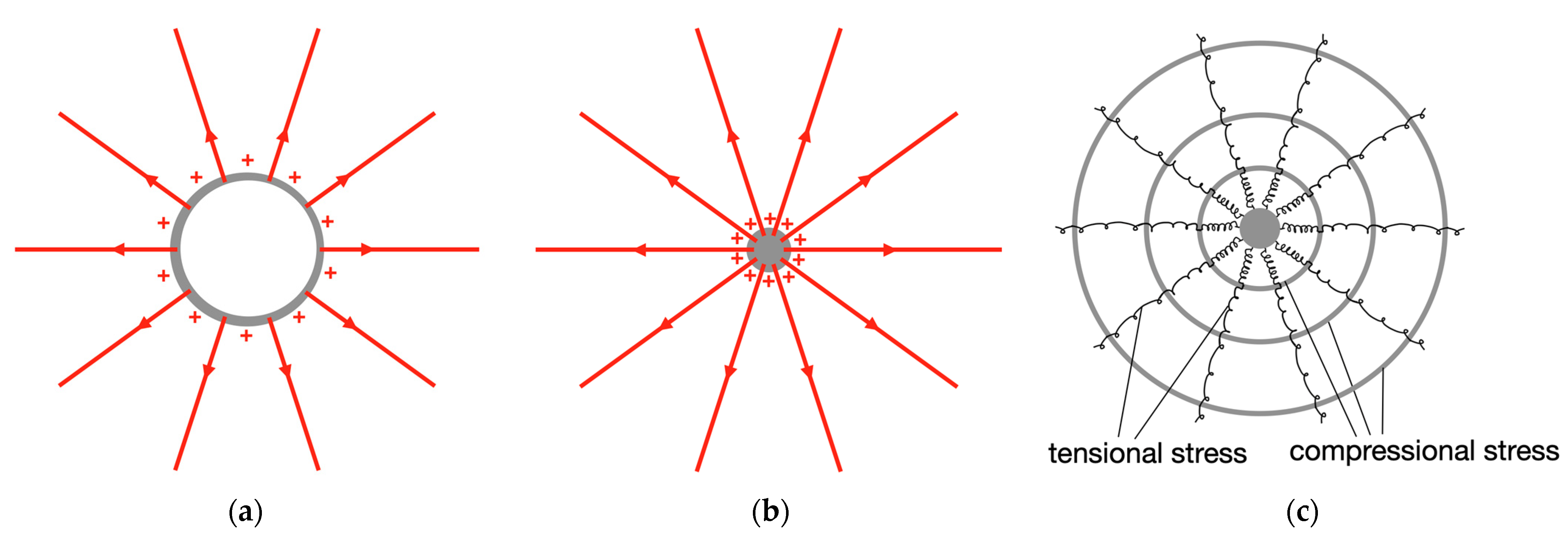
Let us consider a simple system: a hollow sphere on whose surface an electrically positive charge is uniformly distributed, Figure 1a. The interior of the sphere is known to be free of field. If we imagine that the sphere is made of an elastic material, it will inflate when charged.

The traditional actions-at-a-distance description is as follows: the charges repel each other. However, one can see the inappropriateness of this description; the connecting straight lines between all “repulsing” parts of the sphere’s surface run through the field-free interior of the sphere.

A better description is as follows: the field is under tensile stress in the direction of the field lines. The field lines end on the surface of the sphere. The tension is passed on to the sphere. Therefore, instead of “the charged parts of the sphere repel each other” it is better to say: “The electric field pulls outward on the sphere”.

Let us now imagine that we reduce the size of the sphere while keeping the charge constant, as in Figure 1b. Thereby, the field outside the original sphere does not change, but new field is created inside. We have spent energy to create this additional field. This expended energy is stored in the newly generated field. The energy density in the electric field can be easily calculated:

$${\rho }_E=\frac{{\epsilon }_0}{2}{E}^2.$$

(3)

To illustrate the distribution of pressure and tension, let us replace the field with material components: an arrangement of elastic springs and rigid rings, as seen in Figure 1c. The springs are under tensile stress. The farther a spring is from the center, the less the spring is tensioned. As a consequence, the rings are under compressive stress, just as the field is under compressive stress transverse to the field line directions.

4.2. Mechanical Stress within the Gravitoelectric Field

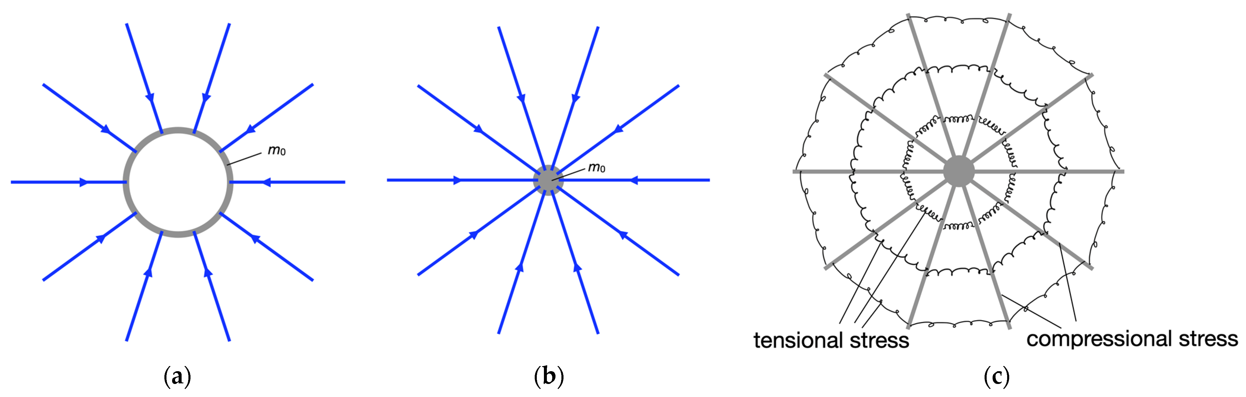
We transfer our reasoning to the gravitational field. We consider a thin spherical shell of mass $m_0$, as in Figure 2a. Similar to its electric analogue, it is field-free in its interior. We know that it has a tendency to shrink. It is prevented from doing so because it is made of a solid material.

Again, we do not want to use the actions-at-a-distance language and we describe the situation in this way: the field pushes on the spherical shell from the outside. We see that there must be compressive stress in the direction of the field lines. Correspondingly, tensile stress prevails in the transverse direction. It is

$${\sigma }_{\parallel }=-\frac{{\epsilon }_{\mathrm{g}}}{2}{g}^2$$

(4)

And

$${\sigma }_{\perp }=\frac{{\epsilon }_{\mathrm{g}}}{2}{g}^2$$

(5)

where we have used the abbreviation

$${\epsilon }_{\mathrm{g}}=\frac{1}{4\pi G}.$$

(6)

These stresses are summarized in the stress tensor of the GEM field, the analogue of the Maxwell stress tensor.

Again, for comparison, we consider a small sphere of the same mass $m_0$, as in Figure 2b. The field outside the region of the original hollow sphere is the same as that of the small sphere. Again, there is new field inside this region.

If we stick to the idea that energy can be localized, i.e., that we can always specify an energy density, we cannot avoid the conclusion that the field has a negative energy density [12]. It can be calculated:

$${\rho }_E=-\frac{{\epsilon }_{\mathrm{g}}}{2}{g}^2.$$

(7)

Here, too, the stresses can be modeled with a spring model, as in Figure 2c. The radial bars are under compressive stress, the springs under tensile stress.

5. Energy Flow

5.1. Energy Exchange with the Gravitational Field of the Earth

So far, we have been dealing with mechanical stresses in the gravitoelectric field, i.e., stresses whose value is calculated from the field strength $g$, Equations (4) and (5). The gravitomagnetic stresses are smaller by a factor $v^2/c^2$ and are not detectable in simple experiments. Nevertheless, the gravitomagnetic field manifests itself very clearly but not via forces into which the gravitomagnetic field strength enters quadratically but via the energy flow, which contains $b$ linearly. The energy flow density in the electromagnetic field is known to be:

$$S=\frac{1}{{\mu }_0}E\times B.$$

(8)

The GEM analogue is:

$$S=-\frac{1}{{\mathit{\mu }}_g}g\times 4b.$$

(9)

Here we have abbreviated:

$${\mu }_{\mathrm{g}}=\frac{4\pi G}{c^2}.$$

(10)

The mapping of Maxwell’s equations to the corresponding gravitoelectro-magentic ones can be done in different ways. If one decides for the correspondence $B \to b$, then a factor 4 appears in Equation (9).

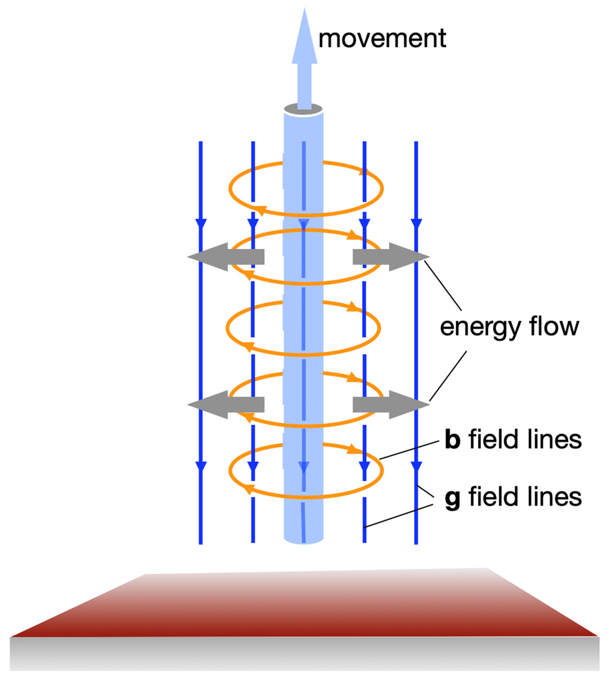
To keep things manageable, we chose a simple geometry, seen in Figure 3: A long rod is moved upwards perpendicularly to the earth’s surface. As is well known, energy is needed for this. The total energy flow distribution is complicated, but what can be easily determined is the energy flow near the surface of the rod [5].

The $g$ field of the rod is so weak compared to that of the earth that we need not consider it.

The field strength of the $b$ field is [6]:

$$b\left(r\right)={\mu }_{\mathrm{g}}·\frac{I_m}{2\pi r}.$$

(11)

Here, $I_m$ is the mass current strength, and $r$ the distance from the middle axis.

Together with the magnitude $g$ of the field strength of the $g$ field of the earth we find for the magnitude of the energy current density:

$$S=\frac{1}{{\mu }_{\mathrm{g}}}g·4b.$$

(12)

Assuming we pull the rod from the top, the energy flows within the material of the rod from top to bottom and successively exits to the sides into the field.

This outgoing energy is said to be the “potential energy of the body”. This is a kind of statement we want to avoid. We prefer to say: it is energy that goes into the gravitational field and, thereby, weakens the field. We remember: one needs energy to create field-free space or to weaken a field.

5.2. A Closed Energy Circuit

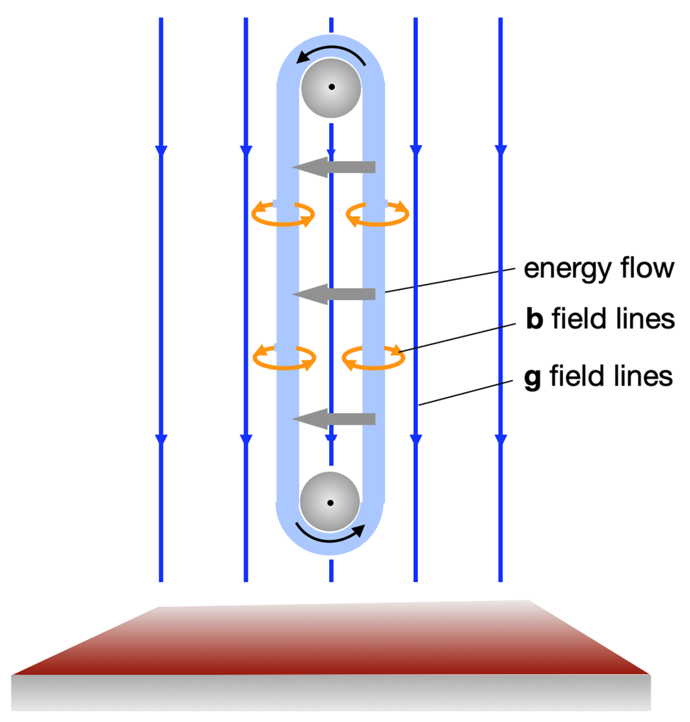
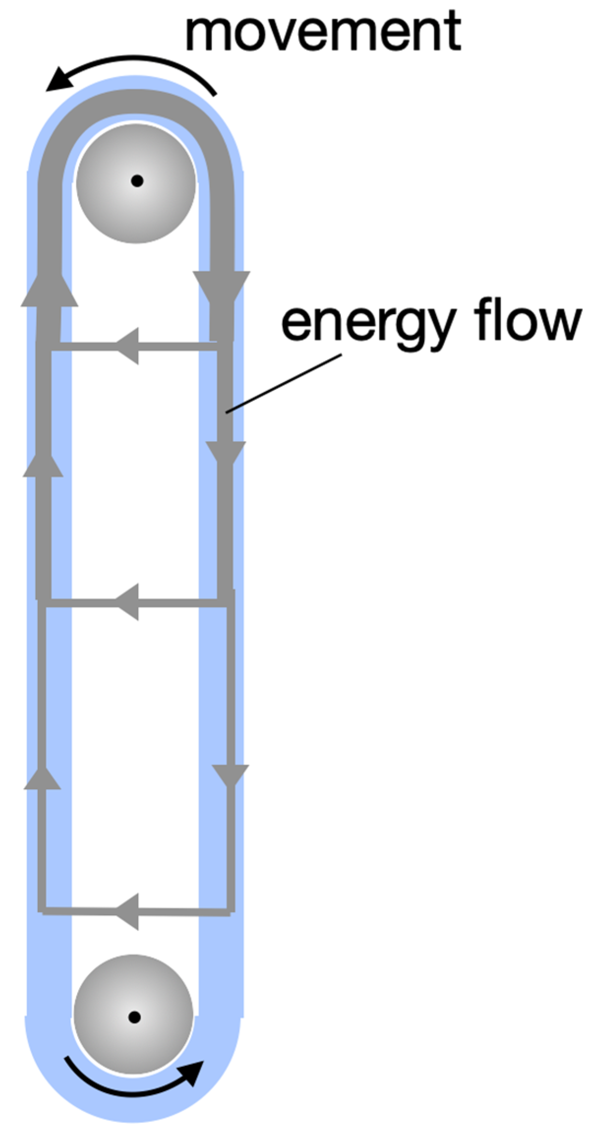
Next, we consider the arrangement of Figure 4. A heavy rope runs over two pulleys. (One can also imagine that it is water flowing in a pipe).

We now set the rope in motion. It, thereby, traverses only equilibrium states. The part of the rope (or of the water), that moves downwards constantly receives energy from the gravitational field. (It is said that its potential energy decreases.) The right part, which moves upwards, releases energy to the field. The energy that the left part receives from the field is transported by the rope over the pulley to the right part. We, thus, have a stationary, closed circuit for the energy. Figure 5 (statt 9) shows the energy flow schematically.

We are interested in that part of the path of the energy that proceeds within the gravitational field.

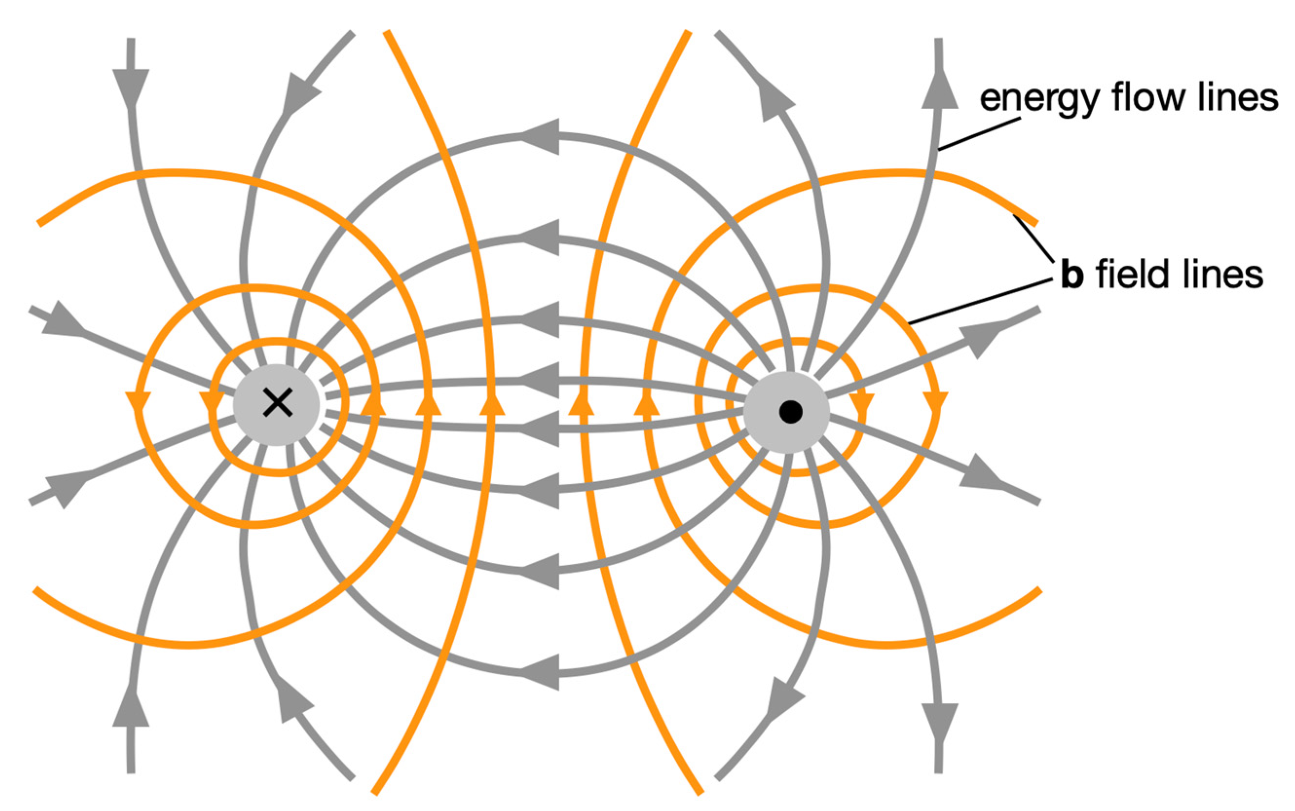
For this purpose, we need the field strength distributions of the $g$ and the $b$ field. The $g$ field is very simple, namely, homogeneous (we neglect the contribution to $g$ provided by the rope). The $b$ field is an old acquaintance: its field line pattern has the same shape as that of two wires through which an electric current flows in opposite directions, i.e., that of an ordinary two-wire cable, as seen in Figure 6. Since $g$ is homogeneous, the vector multiplication $g\times b$ is simple: the streamlines of the energy are orthogonal to the $b$ field lines.

Thus, it can be seen that the energy transport is localized to the vicinity of the two sections of the rope.

We have, thus, obtained the energy flow distribution in the gravitational field for an everyday, large effect.

6. Conclusions

We have seen that the energy densities in the GEM field are negative and that the energy flows in the gravitoelectromagnetic field have the opposite direction compared to those in the electromagnetic field.

The gravitomagnetic field seems to be hardly noticeable. This is true as far as it manifests itself as a force, i.e., as a momentum current. On the other hand, it manifests itself clearly in the energy current. This is understandable: in the momentum current, the gravitomagnetic field strength enters quadratically, in the energy current, linearly (together with the gravitoelectric field strength).

How can we deal with GEM in the classroom?

First, a recommendation for both school and university has to do with the language we use and, thus, with the conceptual models we form of the real world.

When we address processes that are traditionally described in terms of potential energy, we say something similar to: when you move two bodies against each other, they exchange energy with the gravitational field. Energy flows into or out of the gravitational field. In this process, energy is needed to create field-free space. It can also be that the energy, as in our last example, only flows through the gravitational field. Therefore, it does not increase or decrease anywhere within the field.

As far as the university is concerned, we recommend introducing not only the field strength g but also the gravitomagnetic field strength b, as well as the analogous Maxwell equations. One should not do this in the introductory mechanics lecture, because at that time the students are not yet familiar with Maxwell’s theory. We, therefore, suggest devoting about two lessons of the lecture to electromagnetism. Not only does it give the students a new view on gravity, it is also a good exercise for dealing with Maxwell’s theory.