Proceeding Paper

Comparison between Three Paradigms of General Relativity †

by
Kareema Al Hosni
*,‡ and
Mudhahir Al Ajmi
*,‡
Physics Deprtment, Sultan Qaboos University, P.O. Box 36, Al khoudh 123, Muscat, Oman
*
Authors to whom correspondence should be addressed.
Presented at the 1st Electronic Conference on Universe, 22–28 February 2021; Available online: https://ecu2021.sciforum.net/.
These authors contributed equally to this work.
Phys. Sci. Forum 2021, 2(1), 48; https://doi.org/10.3390/ECU2021-09280
Published: 22 February 2021
(This article belongs to the Proceedings of The 1st Electronic Conference on Universe)

Abstract

:
Gravity formulated as a classical gauge theory is based on the Mach principle in terms of curvature scalar R by A. Einstein. The original idea of Einstein limits the gravity to act as a curvature in spacetime. However, there exist other possible classical fields such as torsion and non-metricity. The aim of this paper is to make a compatible comparison between three paradigms: Gravity as curvature via Einstein–Hilbert action, Teleparallel Gravity (TEGR) and Coincidence Gravity (CGR). In TEGR, a flat spacetime is considered as well as an asymmetric connection metric. In CGR, gravity is constructed in an equally flat, tortionless spacetime, which is ascribed to non-metricity. The strength and weakness of each formulation is tested in the framework of a homogeneous and isotropic cosmological background. Mainly, the equivalence between GR and TEGR is examined at the level of equation of motion. Furthermore, we study the interactions between dark energy, dark matter and radiation, and the stability of these models is explored. The implications of the interaction were tested in both early and late epochs of the universe. It has been found that mostly there is a similarity of description of the evolution of the universe provided by GR and TEGR, while CGR always showed different description.

1. Introduction

Modifications of general relativity (GR) was motivated by the discovery of the accelerated expansion of the universe. Therefore, a number of theories have been established based on particular approaches [1]. GR describes the geometric properties of spacetime, taking the curvature as a fundamental geometrical object. The best-known representation of GR at which gravity is formulated with the dynamic of curvature in spacetime by the Hilbert action
S = 1 2 κ 2 d 4 x g R + S m .
Here, S m is the mater action, which is defined as S m = L m g d 4 x and κ 2 = 8 π G and it is called the gravitational coupling [2].
Although GR is a very elegant theory that succeeds in describing many phenomena, it still suffers from flaws that invoke the demand for finding an alternative description for gravity. One of the problems that GR faces is the cosmological constant problem. Einstein equations bring out the scenario of dark energy by setting the cosmological constant. The cosmological constant is the simplest interpretation for dark energy that represents a constant energy density of empty space. Nevertheless, there is an incompatibility in the theoretical and observational calculation of the cosmological constant. The cosmological constant problem has serious impacts in the description of the evolution of the universe.
Other equivalent geometrical descriptions of gravity are Teleparallel Gravity and Coincidence General Relativity. The former is based on torsion and the later is based on non-metricity.
  • Teleparallel Gravity
Teleparallel Gravity is based on torsion and vanishing curvature. It is mapped in non-Riemmanian geometry called Wietzenböck [3]. Tetrads basis vector e μ i is the essential quantity in Teleparallel gravity. They are defined by [4]
g μ ν = e μ i e ν j η i j
where η i j is flat Minkowski metric. Teleparallel is extended to what is called f ( T ) gravity, where f ( T ) indicates an arbitrary function for torsion, such that it reduces to TEGR if f ( T ) = T [5]. General action for f ( T ) gravity reads
S = 1 2 κ 2 d 4 x e ( T + f ( T ) ) + S m .
Here, S m is the action of matter, and T is
T = S σ μ ν T μ ν σ ,
where
S σ μ ν = 1 2 ( K σ μ ν + δ σ μ T ρ ρ ν δ σ μ T ρ ρ μ ) K σ μ ν = 1 2 ( T σ μ ν T σ ν μ T σ μ ν ) .
  • Coincidence General Relativity
A further modification was made by formulating GR via the non-metricity. The non-metricity is the fundamental object in Coincidence General Relativity, which is the derivative of the metric tensor. It is attributed to flat and torsion-free spacetime which implies that vectors stay parallel along the space [6]. In Coincidence GR (CGR), the inertial effect vanishes, which means that the connection Γ μ ν σ = 0 [1], and this gives CGR an advantage over GR. Another advantage for CGR is that it can be achieved without the need of boundary terms [2]. The general action for a non-metricity scalar is:
S = d 4 x g Q + S m .
Evidences show that we now live at a special cosmic epoch; which is a transition from decelerating to accelerating universe and from matter-dominated to dark-energy-dominated universe [7]. The reason for this is that the volume of space increases as the universe expands, so the density of matter decreases. On the other hand, the density of dark energy does not change as the universe expands. Hence, the density of dark energy is higher than that of matter in the current time. There are several models that can be presumed for dark energy. For instance, cosmological constant, quintessence and phantom energy.
In order to describe the phenomenon of dark energy, numerous models has been introduced which are based on the interaction of dark energy with dark matter or any other types of fluid. As established in GR, the cosmological constant is a simple solution to dark energy. Quintessence and phantom energy are alternative models to describe the dark energy, which represent components that have negative pressure. They are dynamical quantities that can be characterized by their equation of state [8]. Most of models which represent quintessence have w < 1 3 , phantom energy w < 1 and cosmological constant has w = 1 [9]. The larger the value of w, the smaller its accelerating. The cosmological constant does not evolve with time, whereas the quintessential does [8].
In this paper, we are interested in comparing the evolution of the universe described by the three theories (GR, TEGR and CGR). The paper is organized as follows: In Section 2, the equations and mathematical models used in the project are introduced. Section 3 represents the cosmological models and stability analysis of GR, TEGR and CGR, respectively, along with the results for each paradigm. In the last Section 4, the numerical solutions plots that describe the evolution of the universe are shown.

2. Materials and Methods

We investigate the cosmological dynamics for the three theories; GR, TEGR and CGR. Considering Friedmann–Lemaitre–Roberson–Walker (FLRW) metric:
g μ ν = d i a g ( 1 , a ( t ) 2 , a ( t ) 2 , a ( t ) 2 ) ,
where a ( t ) is the scale factor, the Friedmann equations take a general form as
3 H 2 = κ 2 ρ i , 2 H ˙ = κ 2 ( P i + ρ i ) .
Here H is the Hubble, where H = a ˙ ( t ) a ( t ) . Furthermore, P i is pressure and ρ i is the density. The pressure and density are represented here generally. However, they are considered to represent the pressure and density mainly for three types of fluids, which are dark energy, dark matter and radiation, respectively;
P i = P Λ + P m + P r + ρ i = ρ Λ + ρ m + ρ r +
Because these fluids are taken to be perfect fluids, we can write P = w ρ , where w is the equation of state parameter. For dark matter w m = 0 , for radiation w r = 1 3 and w λ is for dark energy. The corresponding continuity equations for the three fluids:
ρ ˙ Λ + 3 H ( ρ Λ + P Λ ) = β Λ , ρ ˙ m + 3 H ( ρ m + P m ) = β m ρ ˙ r + 3 H ( ρ r + P r ) = β r ,
where β is the interaction parameter that describes how the considered fluids interact with each other such that β Λ + β m + β r = 0 . For this work, we constructed two models of interaction:
  • Model-I of interaction
    β Λ = α Λ H 3 κ 2 Ω Λ Ω m
    β m = α m H 3 κ 2 Ω r Ω m
    β r = α r H 3 κ 2 Ω m ( Ω Λ Ω r ) ,
  • Model-II of interaction
    β Λ = α Λ H 3 κ 2 Ω r ( Ω Λ Ω m )
    β m = α m H 3 κ 2 Ω m ( Ω Λ Ω r )
    β r = α r H 3 κ 2 Ω Λ ( Ω m Ω r ) .
The stability of the corresponding dynamical systems will be analyzed around the critical points. The dynamical system is ascribed to a dimensionless density parameter Ω , which is defined as:
Ω = ρ ρ c .
Here, ρ c is the critical density. Henceforth, we have:
ρ Λ = 3 H 2 κ 2 Ω Λ , ρ m = 3 H 2 κ 2 Ω m , ρ r = 3 H 2 κ 2 Ω r .
Here Ω Λ , Ω m and Ω r are density parameters corresponding to dark energy, dark matter and radiation, respectively, whereas α Λ , α m and α r are coupling constants. To construct a dynamical system of Ω instead of ρ , we use the e-folding parameter N = ln ( a ) = ln ( 1 + z ) , so that the derivative density parameter will be taken with respect to N, ( d Ω d N ). The Jacobi stability of dynamical systems will be applied. To apply the Jacobi stability, consider
d Ω d N = f ( Ω ) .
The function f is called a vector field. A point Ω is a fixed point or critical point for which f ( Ω ) = 0 . The linearization is implemented by Hartman theorem, which states that the differential system and the linearized system are topologically equivalent, if they are treated locally [10]. To linearize the vector field around this point, we define the Jacobian matrix J such that [3]
J = ( D f ) | p = f i Ω i | p
and specifically for our study, we have
f 1 Ω Λ f 1 Ω m f 1 Ω r f 2 Ω Λ f 2 Ω m f 2 Ω r f 3 Ω Λ f 3 Ω m f 3 Ω r
where f 1 = d Ω Λ d N , f 2 = d Ω m d N and f 3 = d Ω r d N .

3. Numerical Solutions

3.1. General Relativity

Dynamical Systems and Stability Analysis

Considering Equation (7), the pressure and the density are
ρ i = ρ Λ + ρ m + ρ r P i = P Λ + P m + P r .
We constructed the system of equations of the density parameter according to the two models of interaction and find the corresponding fixed points. We have:
  • Model I of interaction
Now, we write the dynamical system of density parameter equations corresponding to our Model-I of interaction as
d Ω Λ d N = 3 Ω Λ [ ( 1 + w Λ ) Ω Λ + Ω m + 4 3 Ω r ] 3 ( 1 + w Λ ) Ω Λ + α Λ Ω Λ Ω m 3
d Ω m d N = 3 Ω m [ ( 1 + w Λ ) Ω Λ + Ω m + 4 3 Ω r ] 3 Ω m + α m Ω r Ω m 3
d Ω r d N = 3 Ω r [ ( 1 + w Λ ) Ω Λ + Ω m + 4 3 Ω r ] 4 Ω r + α r Ω m ( Ω Λ Ω r ) 3 .
Table 1 summarizes the solutions of the above differential equations where four critical points were found for the first model of interaction at GR. These critical points are conditionally stable. Point A 1 is stable if w Λ < 1 , whereas B 1 is stable if w Λ > 3 and a > 9 . For point C 1 , it is stable if w Λ > 1 9 a , a < 3 . Then, D 1 will be stable when w Λ < 1 .
  • Model II of interaction
The system of density parameter equations in this model are:
d Ω Λ d N = 3 Ω Λ [ ( 1 + w Λ ) Ω Λ + Ω m + 4 3 Ω r ] 3 ( 1 + w Λ ) Ω Λ + α Λ Ω r ( Ω Λ Ω m ) 3
d Ω m d N = 3 Ω m [ ( 1 + w Λ ) Ω Λ + Ω m + 4 3 Ω r ] 3 Ω m + α m Ω m ( Ω Λ Ω r ) 3
d Ω r d N = 3 Ω r [ ( 1 + w Λ ) Ω Λ + Ω m + 4 3 Ω r ] 4 Ω r + α r Ω Λ ( Ω m Ω r ) 3 .
Table 2 shows the critical points gained from applying the second model of interaction on GR. We have point A 2 is stable if it satisfies the condition w Λ > 1 , while point B 2 is not stable since we have λ 3 = 4 . The last point, C 2 , is stable under the conditions w Λ < ( 1 3 + 1 9 a ) and a 12 .

3.2. Teleparallel Equivalence of General Relativity

3.2.1. Cosmological Model

Now, we investigate the cosmological dynamics for the model based on TEGR. The torsion scalar is:
T = 6 H 2 .
Then, Friedman equations are:
3 H 2 = κ 2 ( ρ + ρ T ) 2 H ˙ = κ 2 [ ( ρ + P ) + ( ρ T + P T ) ]
where P T and ρ T are the pressure and density of the torsion field. Therefore, beside Equation (9), we will have the continuity equation of the torsion field:
ρ ˙ T + 3 H ( ρ T + P r ) = 0

3.2.2. Dynamical Systems and Stability Analysis

  • Model I of interaction
For TEGR, the system of density parameter equations corresponding to the first model of interaction (model I):
d Ω Λ d N = 3 Ω Λ [ ( 1 + w Λ ) Ω Λ + Ω m + 4 3 Ω r ] 3 ( 1 + w Λ ) Ω Λ + α Λ Ω Λ Ω m 3
d Ω m d N = 3 Ω m [ ( 1 + w Λ ) Ω Λ + Ω m + 4 3 Ω r ] 3 Ω m + α m Ω r Ω m 3
d Ω r d N = 3 Ω r [ ( 1 + w Λ ) Ω Λ + Ω m + 4 3 Ω r ] 4 Ω r + α r Ω m ( Ω Λ Ω r ) 3
d Ω T d N = 3 Ω T [ ( 1 + w Λ ) Ω Λ + Ω m + 4 3 Ω r ] .
The table below (Table 3) shows the critical points of TEGR. It was observed that all critical points are stable under some conditions. Notice that conditions that does not match the fact that w Λ ranges from 1 3 to 1 cannot be met. The interaction parameter a is selected to be in order of unity.
  • Model II of interaction
For the second model of interaction, the equations of density parameters are
d Ω Λ d N = 3 Ω Λ [ ( 1 + w Λ ) Ω Λ + Ω m + 4 3 Ω r ] 3 ( 1 + w Λ ) Ω Λ + α Λ Ω r ( Ω Λ Ω m ) 3
d Ω m d N = 3 Ω m [ ( 1 + w Λ ) Ω Λ + Ω m + 4 3 Ω r ] 3 Ω m + α m Ω m ( Ω Λ Ω r ) 3
d Ω r d N = 3 Ω r [ ( 1 + w Λ ) Ω Λ + Ω m + 4 3 Ω r ] 4 Ω r + α r Ω Λ ( Ω m Ω r ) 3
d Ω T d N = 3 Ω T [ ( 1 + w Λ ) Ω Λ + Ω m + 4 3 Ω r ] .
Similarly, for TEGR the stability of the model is examined. Table 4 summarizes the solutions of the above differential equations.The four fixed points were obtained. The first point, is stable, provided that w Λ > 1 . It is clear that the second point B 2 is unstable because it has a positive eigenvalue λ 3 = 4 . For C 2 , it is also conditionally stable, as it is stable, if the following conditions are satisfied:
w Λ < 1 3 + a 9   for   a 12
w Λ < 1   for   a > 12
and the equation of state reads
w e f f = P t o t ρ t o t = w Λ Ω Λ + 1 3 Ω r Ω T Ω Λ + Ω r + Ω m + Ω T = w Λ Ω Λ + 1 3 Ω r Ω T 1 + Ω T .

3.3. Coincidence General Relativity

3.3.1. Cosmological Model

Q is the non-metricity scalar such that
Q = 6 H 2 .
Referring to Equation (7), we rewrite the equations in this context as:
3 H 2 = κ 2 ( ρ + ρ Q )
2 H ˙ = 3 H 2 κ 2 ( P + P Q ) .
In the above equations, we point out that ρ = ρ λ + ρ m + ρ r and P = P λ + P r + P m .

3.3.2. Dynamical Systems and Stability Analysis

  • Model I of interaction
The system of differential equation for the second model of interaction are:
d Ω Λ d N = 3 Ω Λ [ 1 Ω Λ + 1 3 Ω r ] 3 ( 1 + w Λ ) Ω Λ + α Λ ( Ω Λ Ω m ) 3
d Ω m d N = 3 Ω m [ 1 Ω Λ + 1 3 Ω r ] 3 Ω m + α m Ω m Ω r 3
d Ω r d N = 3 Ω r [ 1 Ω Λ + 1 3 Ω r ] 4 Ω r + α r Ω m ( Ω Λ Ω r ) 3 .
d Ω Q d N = 3 Ω Q [ ( 1 + w Λ ) Ω Λ + Ω m + 4 3 Ω r ]
In the same manner, three fixed points were found at CGR (Table 5), and again all points should satisfy a given condition to meet the stability.
  • Model II of interaction
d Ω Λ d N = 3 Ω Λ [ 1 Ω Λ + 1 3 Ω r ] 3 ( 1 + w Λ ) Ω Λ + α Λ Ω r ( Ω Λ Ω m ) 3
d Ω m d N = 3 Ω m [ 1 Ω Λ + 1 3 Ω r ] 3 Ω m + α m Ω m ( Ω Λ Ω r ) 3
d Ω r d N = 3 Ω r [ 1 Ω Λ + 1 3 Ω r ] 4 Ω r + α r Ω Λ ( Ω m Ω r ) 3 .
d Ω Q d N = 3 Ω Q [ ( 1 + w Λ ) Ω Λ + Ω m + 4 3 Ω r ]
and the equation of state is
w e f f = P t o t ρ t o t = w Q Ω Q + 1 3 Ω r Ω Q + Ω r + Ω m .
In Table 6, the stability is tested around four points. First, A 2 is stable when w Λ > 0 . Second, B 2 is stable if w Λ > 1 3 + 1 9 a for a < 3 .

4. Results and Discussion

In this section, we elaborate the obtained results in plots for different paradigms and different models in each of them. We compare the results between each other and interpret the ability of each model to explain the cosmos.

4.1. Numerical Solutions and Evolutionary Plots

4.1.1. Model-I of Interaction
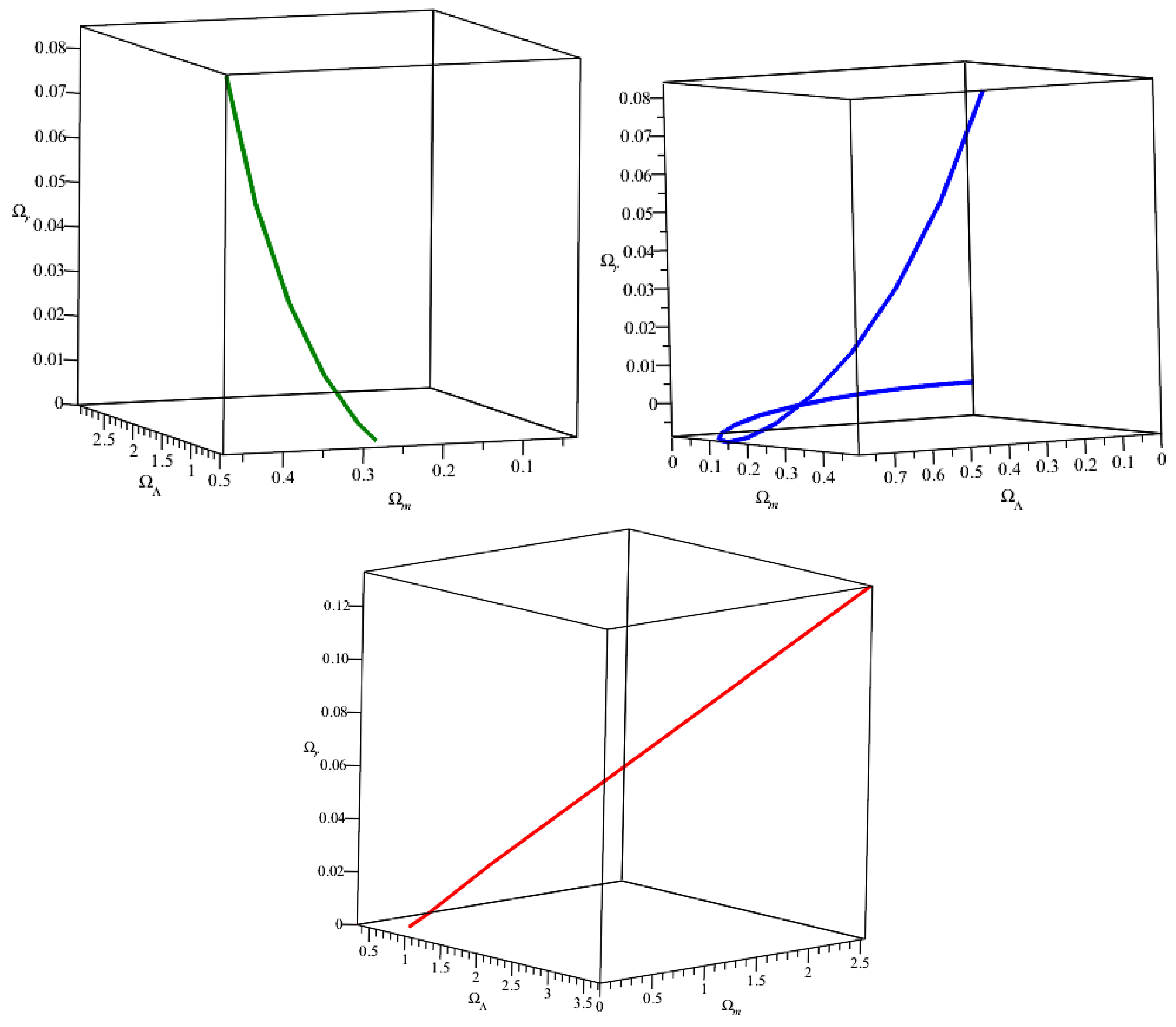
The figures below (Figure 1), obtained as three-dimensional plots from numerical solutions of dynamical system of the density parameter, show how different Ω ’s of the considered fluids are related to each other in model I.
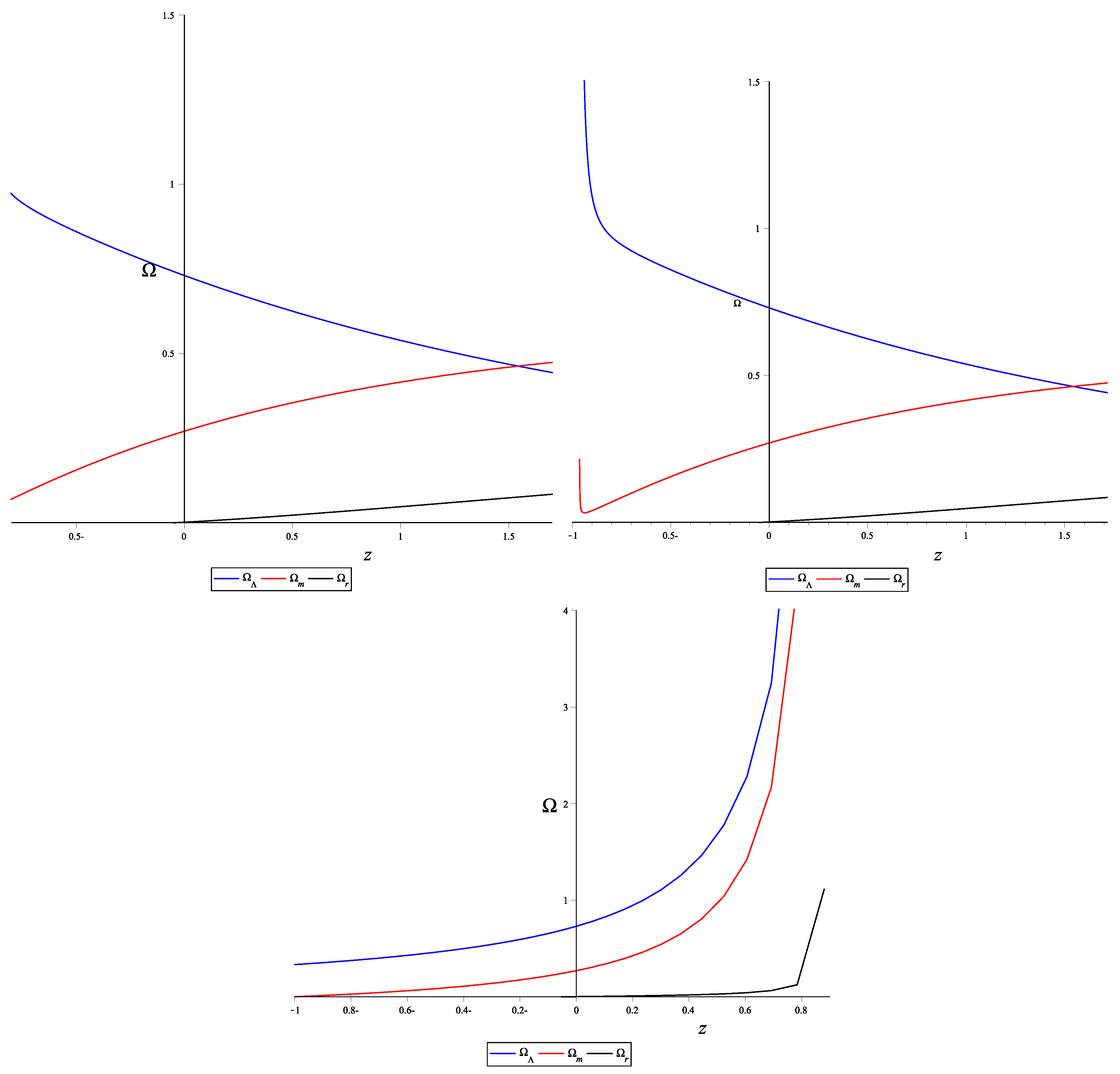
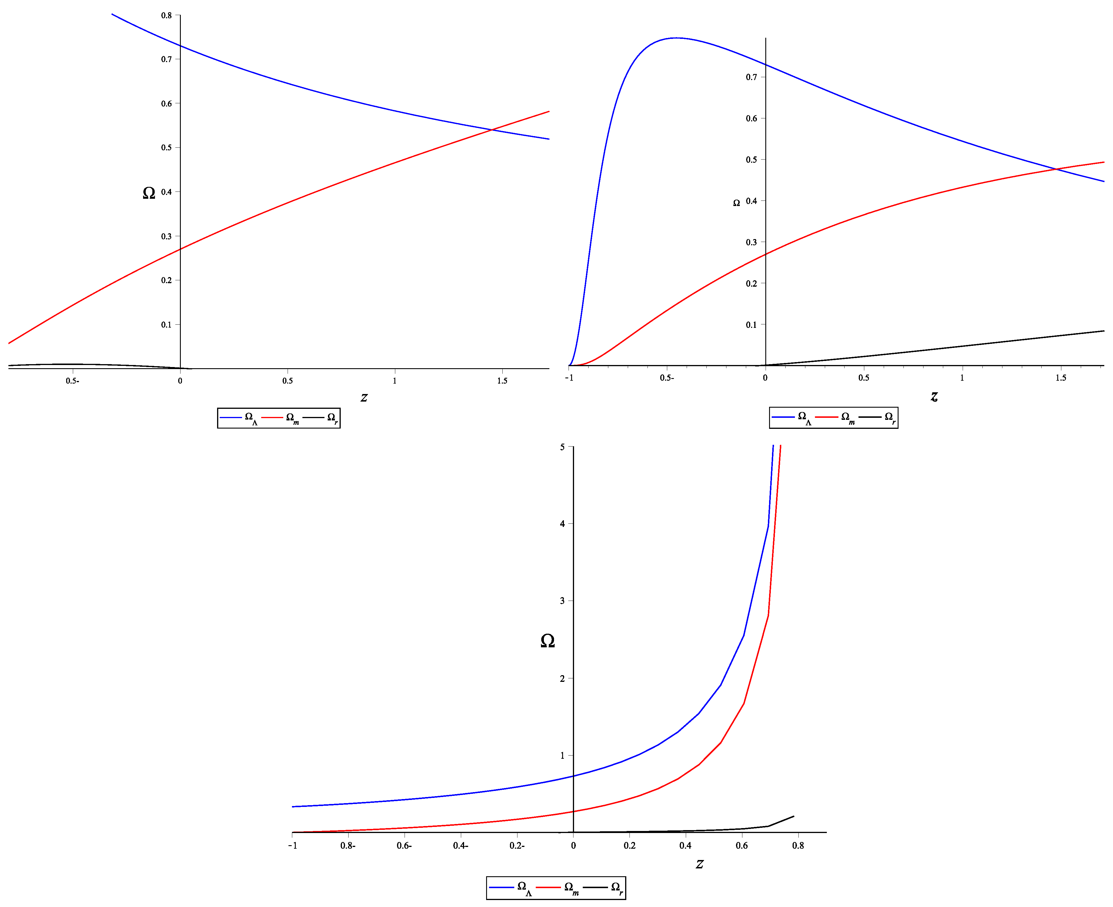
In Figure 2, it was observed that the densities in GR (left) and TEGR (middle) demonstrate nearly similar behavior. There is a point in both figures where dark energy and dark matter acquired the same density in the early time. This is observed at z 1.53 and it indicates an equilibrium point. After this point, the dark energy keeps increasing in later times, while dark matter started to decrease. The density of radiation evolved in the past, However it decreases at z 0.05 and vanishes in the future. On the other hand, for Coincidence General Relativity (right), all of the three ingredients (dark energy, matter and radiation) decrease rapidly with time.
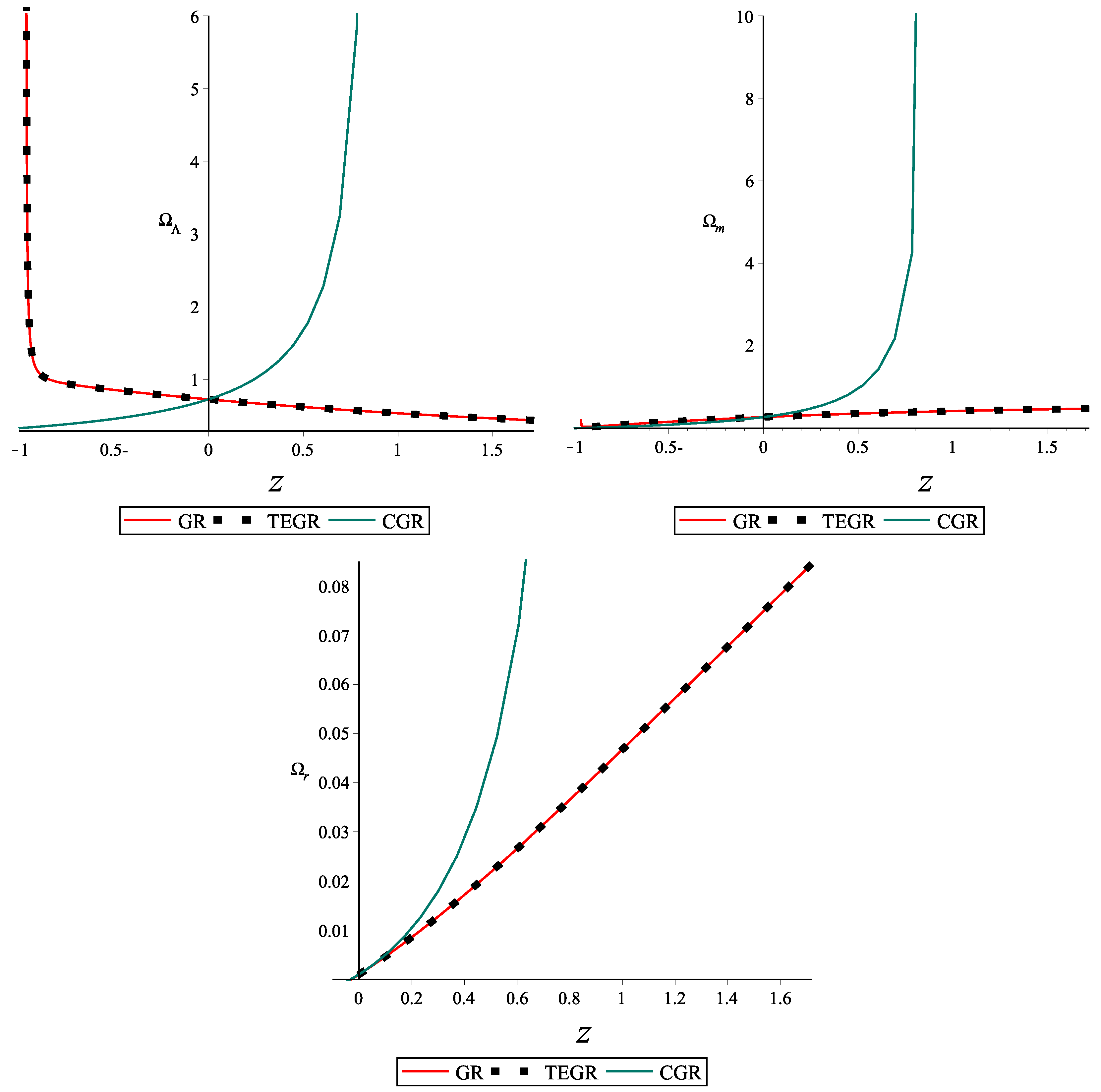
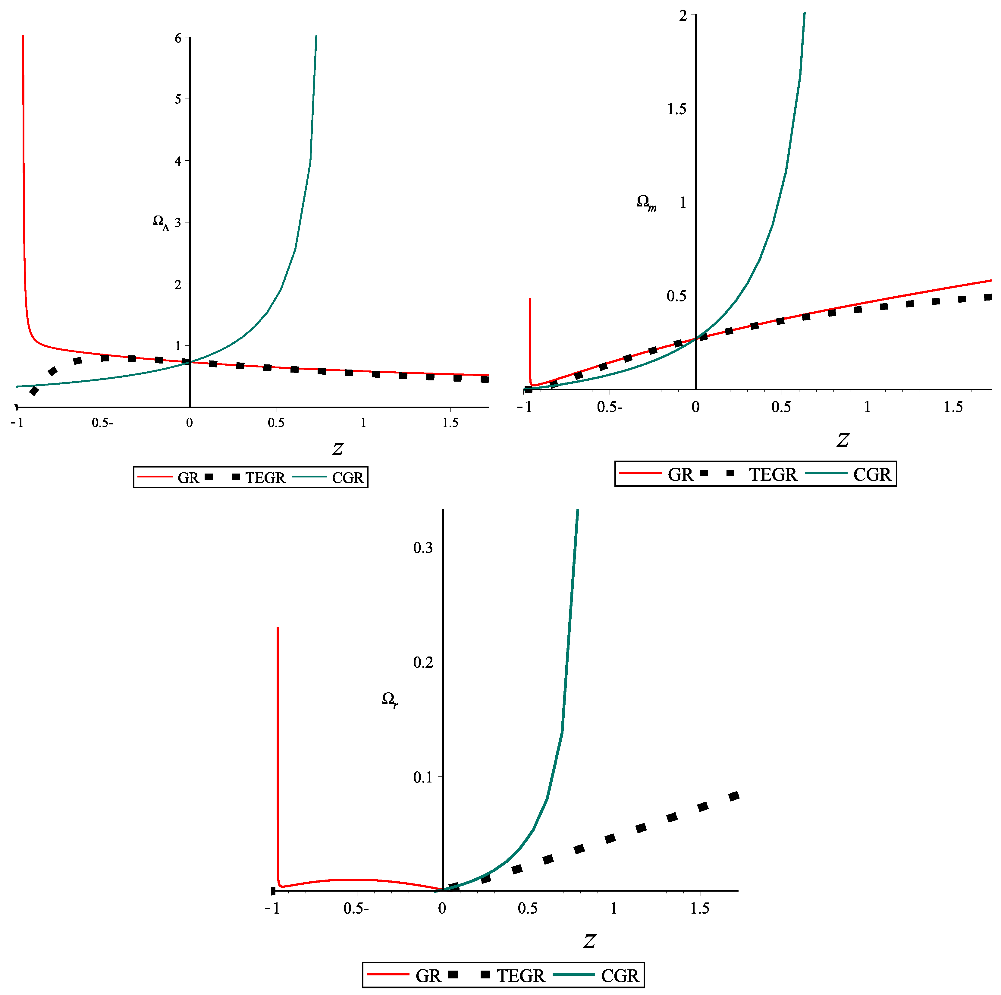
To easily raise a comparison between the three theories, the following plots show each fluid density in separately.
It is noticed in Figure 3 that densities ( Ω Λ , Ω m , Ω r ) described by GR (left) and TEGR (middle) exhibit the same behavior, whereas fluids described by CGR (right) shows different behavior. For all fluids, all three paradigms match at z = 0 , which represents the present time.
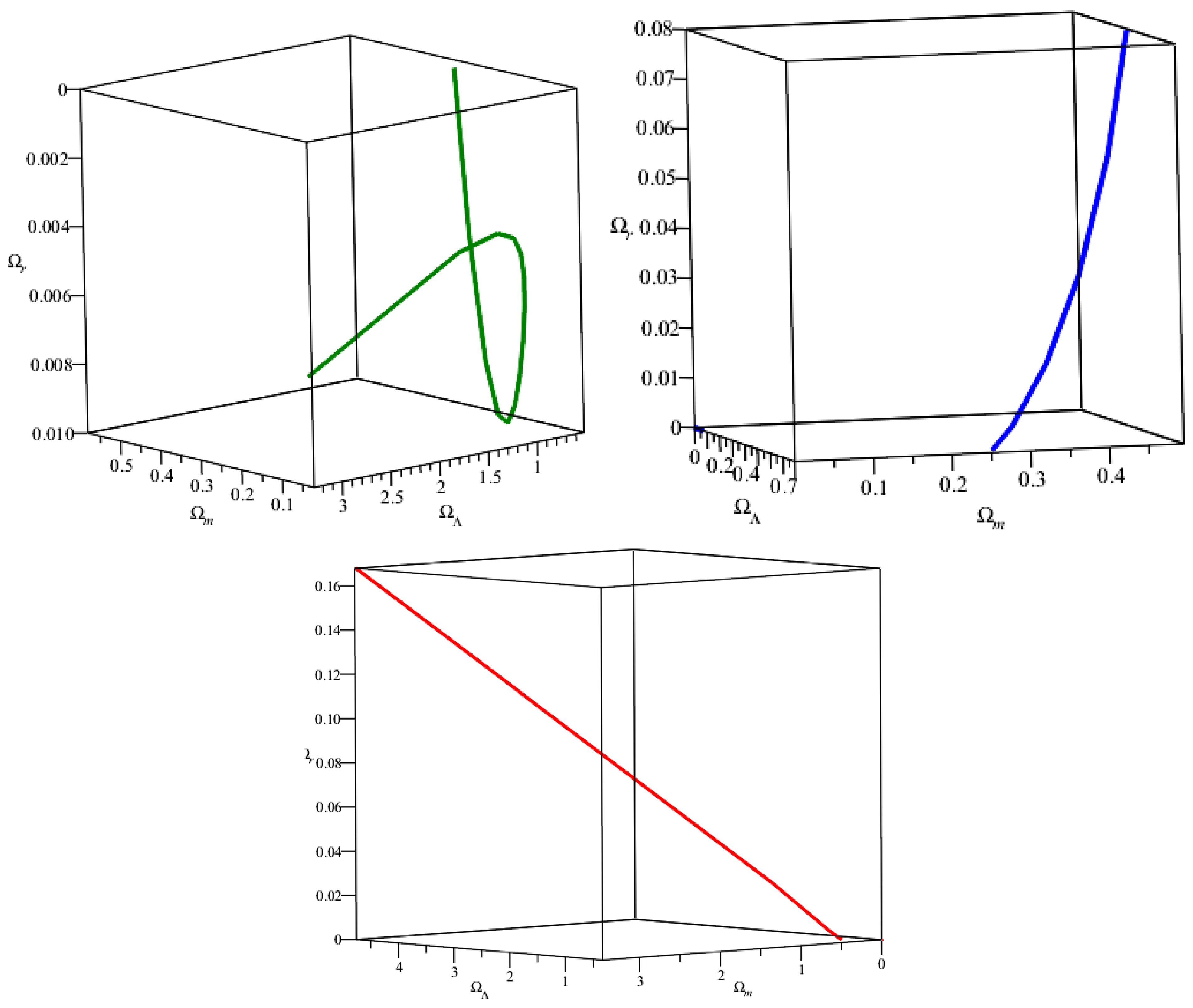
4.1.2. Model-II

Here, numerical solutions of density parameters were obtained to describe the behavior of fluids under the consideration of the second model of interaction.
Figure 4 represents three-dimensional plots of Ω λ versus Ω m versus Ω r for GR, TEGR and CGR, respectively, from left to right.
Similarly, numerical solutions for density parameter equations were provided for the three theories corresponding to the dark energy dark matter and radiation. In the first graph in Figure 5, we notice that the behavior of the three components in GR do not differ much from model-I of interaction. That is, the dark matter is very large in the early universe, but it may decrease in the future, while dark matter behaves apposite to dark energy. The radiation showed up in the early time epoch with very small amount then fades away. It is worth noting that observations revealed that radiation must exist in the early universe. Therefore, model-II of interaction is not compatible with the description of GR. For TEGR (the middle graph in Figure 5), the dark energy oscillates over time, and it arises from very low values, then increases up to Ω Λ 0.8 , and then it decreases again. Radiation and dark matter increased. According to this model, the early universe consists of dark energy and dark matter, as the radiation component emerged later. However, in CGR, dark energy and dark matter exponentially decrease with time.
The combined plots for the Model-II of interaction are shown in Figure 6. It is worth mentioning that in the later times of the universe, each theory has different evolutionary descriptions. The reason is that it is difficult to provide a reliable explanation for the behavior of the fluids in the future. However, we again notice compatible results from GR and TEGR. In Figure 6, GR and TEGR show a decrease in dark energy in the early times, while CGR shows an exponential increase. Similarly, for dark matter we can see that the lines of GR and TEGR suitably are paired together up to z 1 and go separately beyond this value. Finally, the radiation component is different in each of the three theories.

4.2. Equation of State (EoS)

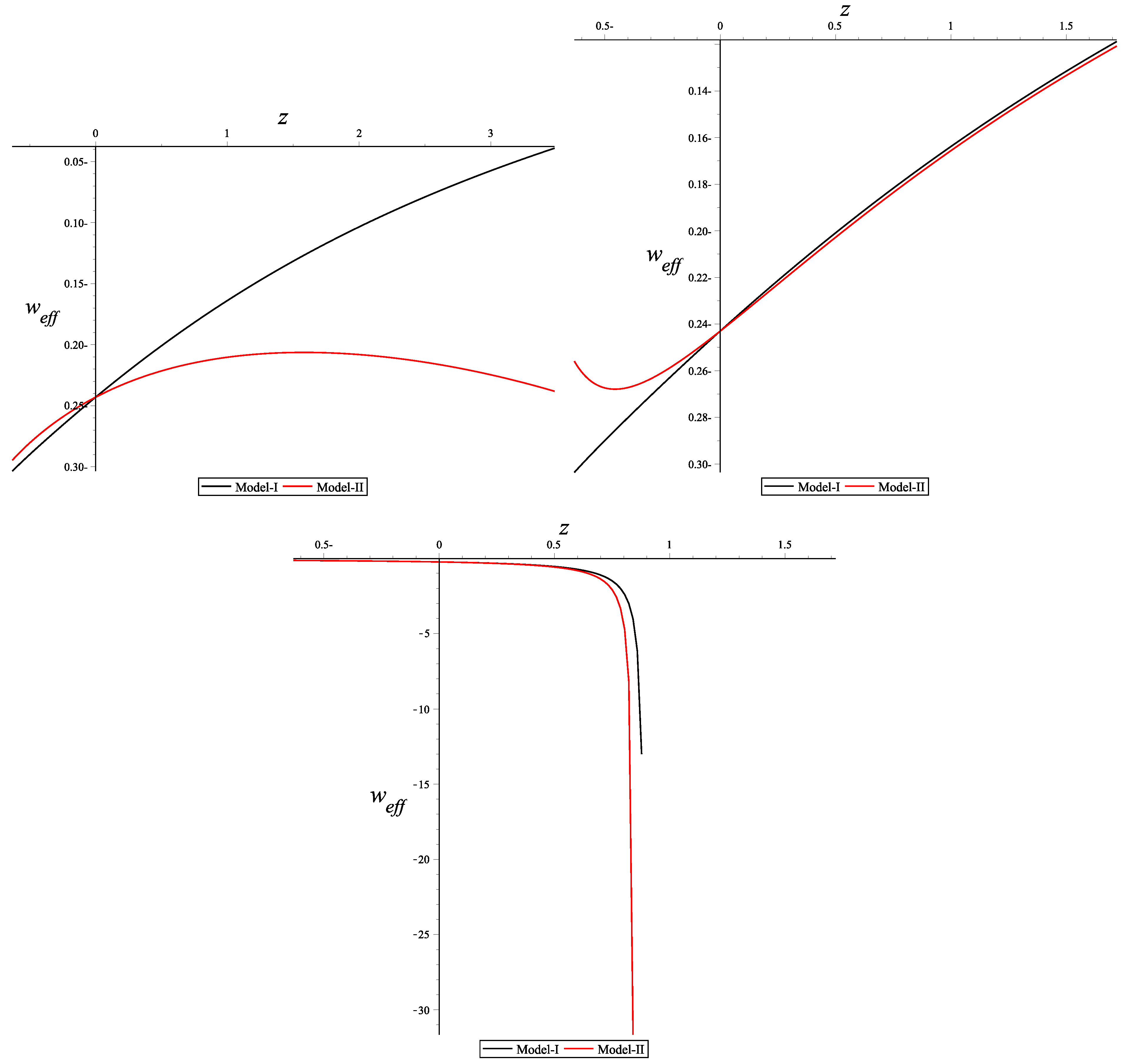
The left-side graph in Figure 7 shows the evolution of the total effective EoS for all the considered fluids (dark energy, dark matter and radiation) described by GR corresponding to the Model-I and Model-II of interaction. We observe that for Model-I, the EoS moves from w e f f = 0.04 to quintessence state ( w e f f < 0.3 ). However, evolution dedicated by the Model-II, w e f f started to evolve from ≈−0.2, then tends to reach the quintessence state. The lines for both models did not cross w e f f = 1 .
The middle figure, represents the EoS devoted by TEGR. At later times ( z < 0.1 ), w e f f for both Model-I and Model-II, EoS evolves from w e f f 0.1 . Then, at later times, EoS for Model-I moves to quintessence, while for Model-II it does not reach the quintessence.
Lastly, the Figure in the right-side represents the EoS as described by CGR. The EoS initially started to evolve from phantom state. After that, it continues to cross w e f f = 1 , which is the cosmological constant state.

5. Conclusions and Future Work

This work investigates the evolution of the universe demonstrated by GR, TEGR and CGR. Three main types of fluid were presumed of which the universe constitutes, namely, the dark energy, dark matter and radiation. We propose two models of interaction to express the way the fluids interact with each other.
From the evolutionary plots obtained from numerical solutions, it was found that describing the universes by curvature in GR and torsion in TEGR lead almost to the same results. However, the non-metricity attributed to CGR gives a distinct explanation. The future of the universe is difficult to predict as the interaction between the fluids is more complicated than our current knowledge, so it requires a more precise model to demonstrate their interactions. Furthermore, the equations of state (EoS) were studied, as they carry information about the acceleration of the universe. It was observed that the EoS for GR and TEGR behaves like quintessence. However, for CGR, the EoS behaves like phantom and crosses the phantom state at w e f f = 1 .
In the subsequent projects, one can study the relation of the observational data with respect to the theory of each of these paradigms and the corresponding models. One can tune the parameters used here according to the data with their errors. Some paradigms and models can fit with certain eras of the universe. This can be left to the future to study.

Author Contributions

K.A.H. performed the analytic calculations and performed the computations. M.A.A. verified the analytical methods and supervised the findings of this work. Both authors have read and agreed to the published version of the manuscript.

Funding

This research received no external funding.

Institutional Review Board Statement

Not applicable.

Informed Consent Statement

Not applicable.

Data Availability Statement

No new data were created or analyzed in this study. Data sharing is not applicable to this article.

Conflicts of Interest

The authors declare no conflict of interest with any person in any organization.

References

  1. Jimenez, J.B.; Heisenberg, L.; Koivisto, T.; Pekar, S. Cosmology in f (Q) geometry. Phys. Rev. D 2020, 101, 103507. [Google Scholar] [CrossRef]
  2. Heisenberg, L. A systematic approach to generalisations of General Relativity and their cosmological implications. Phys. Rep. 2019, 796, 1–113. [Google Scholar] [CrossRef] [Green Version]
  3. Bamba, K.; Momeni, D.; Al Ajmi, M. Phase space description of nonlocal teleparallel gravity. Eur. Phys. J. C 2018, 78, 771. [Google Scholar] [CrossRef]
  4. Jamil, M.; Yesmakhanova, K.; Momeni, D.; Myrzakulov, R. Phase space analysis of interacting dark energy in f(T) cosmology. Cent. Eur. J. Phys. 2012, 10, 1065–1071. [Google Scholar] [CrossRef] [Green Version]
  5. Jamil, M.; Momeni, D.; Myrzakulov, R. Stability of a non-minimally conformally coupled scalar field in F(T) cosmology. Eur. Phys. J. C 2012, 72, 2075. [Google Scholar] [CrossRef] [Green Version]
  6. Lu, J.; Zhao, X.; Chee, G. Cosmology in symmetric teleparallel gravity and its dynamical system. Eur. Phys. J. C 2019, 79, 530. [Google Scholar] [CrossRef] [Green Version]
  7. Jamil, M.; Momeni, D.; Myrzakulov, R. Attractor solutions in f(T) cosmology. Eur. Phys. J. C 2012, 72, 1959. [Google Scholar] [CrossRef]
  8. Steinhardt, P.J. A quintessential introduction to dark energy. Philos. Trans. R. Soc. A 2003, 361, 2497–2513. [Google Scholar] [CrossRef] [PubMed] [Green Version]
  9. Cai, Y.-F.; Saridakis, E.N.; Setare, M.R.; Xia, J.-Q. Quintom cosmology: Theoretical implications and observations. Phys. Rep. 2010, 1, 1–60. [Google Scholar]
  10. Boehmer, C.; Harko, T.; Sabau, S. Stability analysis of dynamical systems-Applications in gravitation and cosmology. Adv. Theor. Math. Phys. 2010, 4, 1145–1196. [Google Scholar] [CrossRef]
Figure 1. Model I: Density parameters of dark energy, matter and radiation for GR, TEGR and CGR.
Psf 02 00048 g001
Figure 2. Model I: Numerical solution for the system of density function versus redshift z for GR, TEGR and CGR.
Psf 02 00048 g002
Figure 3. Model I: Dark energy, matter and radiation densities versus redshift z for GR, TEGR and CGR.
Psf 02 00048 g003
Figure 4. Model II: Density parameters of dark energy, matter and radiation for GR, TEGR and CGR.
Psf 02 00048 g004
Figure 5. Model II: Numerical solution for the system of density function versus redshift z for GR, TEGR and CGR.
Psf 02 00048 g005
Figure 6. Model II: Dark energy, matter and radiation densities versus redshift z for GR, TEGR and CGR.
Psf 02 00048 g006
Figure 7. Effective equation of state w e f f versus redshift z for GR, TEGR and CGR.
Psf 02 00048 g007
Table 1. The stability, critical points and their eigenvalues of GR corresponding to model I of interaction.
Point Ω Λ Ω m Ω r ConditionEigenvalues
A 1 000 w Λ > 1 λ 1 = 3 w Λ 3
B 1 001 w Λ > 3 , a > 9 λ 1 = 9 3 w Λ , λ 2 = 9 a
C 1 010 w Λ > 1 9 a , a < 3 λ 1 = −3 w Λ + 1 3 a , λ 2 = 1 + 1 3 a
D 1 100 w Λ < 1 λ 1 = 3 + 3 w Λ , λ 2 = 3 w Λ 1 , λ 3 = 3 w Λ
Table 2. The stability, critical points and their eigenvalues of GR corresponding to model II of interaction.
Point Ω Λ Ω m Ω r w Λ Eigenvalues
A 2 000 w Λ > 1 λ 1 = 3 w Λ 3 , λ 2 = 3 , λ 3 = 4
B 2 001 w Λ > ( 1 3 + 1 9 a ) , a < 6 λ 1 = 1 3 w Λ + 1 3 a , λ 2 = 1 + 1 6 a , λ 3 = 4
C 2 100 w Λ < ( 1 3 + 1 9 a ) , a 12 λ 1 = 3 w Λ + 3 , λ 2 = 3 w Λ 1 a 3 , λ 3 = 3 w Λ a 6
Table 3. The stability, critical points and their eigenvalues of TEGR corresponding to model I of interaction.
Point Ω Λ Ω m Ω r Ω T w Λ Eigenvalues
A 1 0000 w Λ > 1 λ 1 = 3 3 w Λ , λ 2 = 3 , λ 3 = 4
B 1 0001 w Λ > 1 λ 1 = 3 3 w Λ , λ 2 = 3 , λ 3 = 4
C 1 0010 w Λ > 1 3 , a > 3 λ 1 = 4, λ 2 = 1 3 w Λ , λ 3 = 1 ( 1 3 ) a
D 1 0100 w Λ > a 9 λ 1 = 3 , λ 2 = a 3 1 , λ 3 = 3 w Λ + a 3
E 1 1000 w Λ < 1 λ 1 = 3 + 3 w Λ , λ 2 = 3 w Λ 1 , λ 3 = 3 w Λ
Table 4. The stability, critical points and their eigenvalues of TEGR corresponding to model II of interaction.
Point Ω Λ Ω m Ω r Ω T w Λ Eigenvalues
A 2 0000 w Λ > 1 λ 1 = 3 3 w Λ , λ 2 = 3 , λ 3 = 4
B 2 0010 w Λ > 1 3 a 18 , a < 6 λ 1 = 1 3 w Λ a 6 , λ 2 = 1 + a 6 , λ 3 = 4
C 2 1000 w Λ < 1 3 + a 9 for a 12 , w Λ < 1 for a > 12 λ 1 = 3 + 3 w Λ , λ 2 = 3 w Λ 1 a 3 , λ 3 = 3 w Λ a 6
Table 5. The stability, critical points and their eigenvalues of CGR corresponding to model I of interaction.
Point Ω Λ Ω m Ω r Ω Q ConditionsEigenvalues
A 1 0000 w Λ > 0 λ 1 = 3 w Λ
B 1 0010 w Λ < 1 3 for a > 3 λ 1 = 1 3 w Λ , λ 2 = 1 1 3 a
C 1 1000 1 3 < w Λ < 0 λ 1 = 3 w Λ + 1 3 a , λ 2 = 1 + 1 3 a
Table 6. The stability, critical points and their eigenvalues of CGR corresponding to model II of interaction.
Point Ω Λ Ω m Ω r Ω Q w Λ Eigenvalues
A 2 0000 w Λ > 0 λ 1 = 3 w Λ , λ 2 = 1 , λ 3 = 0
B 2 0010 w Λ > 1 3 + 1 9 a for a < 3 λ 1 = 1 3 w Λ + a 3 , λ 2 = 1 + a 3
C 2 1000 0 < w Λ < 1 a 3 λ 1 = 3 w Λ 1 3 w Λ a , λ 2 = a w Λ +3 w Λ 1 , λ 3 = 9 w Λ
Publisher’s Note: MDPI stays neutral with regard to jurisdictional claims in published maps and institutional affiliations.

