Role of Anisotropy on the Tidal Deformability of Compact Stellar Objects ^†

Abstract

In this paper, we introduce a framework to study the tidal deformation of relativistic anisotropic compact stars. Anisotropic stresses are ubiquitous in nature and widely used in modelling compact stellar objects. Tidal deformability of astrophysical compact objects is a natural effect of gravity, such as one produced by a companion in a binary system. In general relativity, the existence of this measurable effect of gravity can be quantified by their tidal Love numbers (TLN), which characterize the deformability of a neutron star (NS) from sphericity. The tidal deformability or polarizability parameter of an NS depends on its complex internal structure, and hence, the nature of the compact object can be studied by measuring the TLN. We choose a particular solution, which is the anisotropic generalization of the Tolman IV model, as the interior of the compact stellar object. The physical acceptability of the model has been shown graphically by considering the pulsar $4U$ 1608-52 with their current estimated mass and radius. By computing the quadrupole moment, we found that the TLN is dependent on anisotropy of the compact object. We graphically analyze the variation of the TLN against anisotropy for different compact objects with a compactness factor. The numerical value of TLN is given for different compact objects for physically acceptable values of the anisotropic parameter.

1. Introduction

Compact objects are extremely dense astro-physical objects that provide strong gravity and high density, allowing for the study of fundamental physics related to nuclear matter properties. In general, compact objects exist with their binary companion is a natural setup. In this binary setup, a compact star is assumed to be immersed in the tidal field of its companion and hence produce tidal deformation. The possibility of the generation of the gravitational waves during extremely fast rotational motion of a binary system was predicted. Recently, a gravitational wave has been detected by advanced astronomical observations of LIGO and Virgo collaborations from the binary neutron star merger event GW170817 [1]. A neutron star placed in a perturbing external gravitational field is deformed and induces a quadrupole moment, which affects the binding energy of the system and increases the rate of emission of gravitational waves during the late stage inspirals. The recent observational data based on the measurement of the tidal deformability impose a stringent constraint on the allowed equation of state (EOS). In particular, the theoretical prediction of the mass and radius of a neutron star (NS) mostly depends on the nature of the nuclear EOS at supra-nuclear densities. In this context, tidal deformability can be used to study their interiors. The EOS of neutron stars involves their microscopic properties and uniquely determines the macroscopic properties, such as the maximum allowed NS mass, radius and tidal effects. The tidal response is the astrophysical constraints that can be employed as probes of NS properties. It is the astrophysically observable macroscopic property of NS that can be defined as the ratio of the induced multipole moment of a star over the induced tidal field from its companion. The tidal Love number (TLN), which is the ratio of the induced quadrupole moment to the perturbing tidal gravitational field, can be expressed by a relatively simple analytical formula.

On the other hand, the existence of pressure anisotropy, the difference of radial and transverse pressures, is ubiquitous in a compact star. The source of pressure anisotropy in a compact star can be due to various reasons, e.g., pion and kaon condensates [2,3], high density, existence of a solid core or type $3A$ superfluid [4,5], strong magnetic fields [6], a mixture of a perfect and a null fluid, viscosity, and phase transition [7], etc. There are several works available in the literature where incorporating anisotropy into the matter distribution of compact objects in the background of general relativity (GR) has been addressed for various issues of the compact structures [8,9,10,11,12,13,14].

In this paper, we assume a known solution, which is an anisotropic generalization of the Tolman IV model, to describe the compact star. We have calculated the TLN, which actually measures the tidal deformability of the compact object induced by the external field.

2. Physical Features and Tidal Love Number

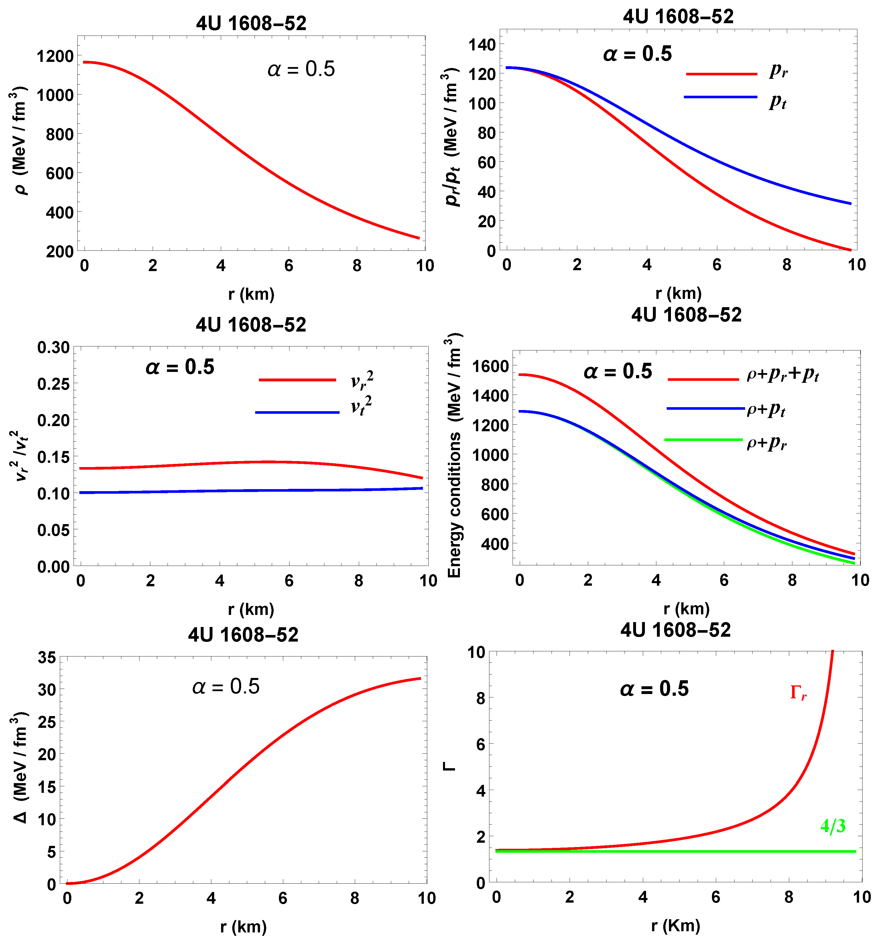
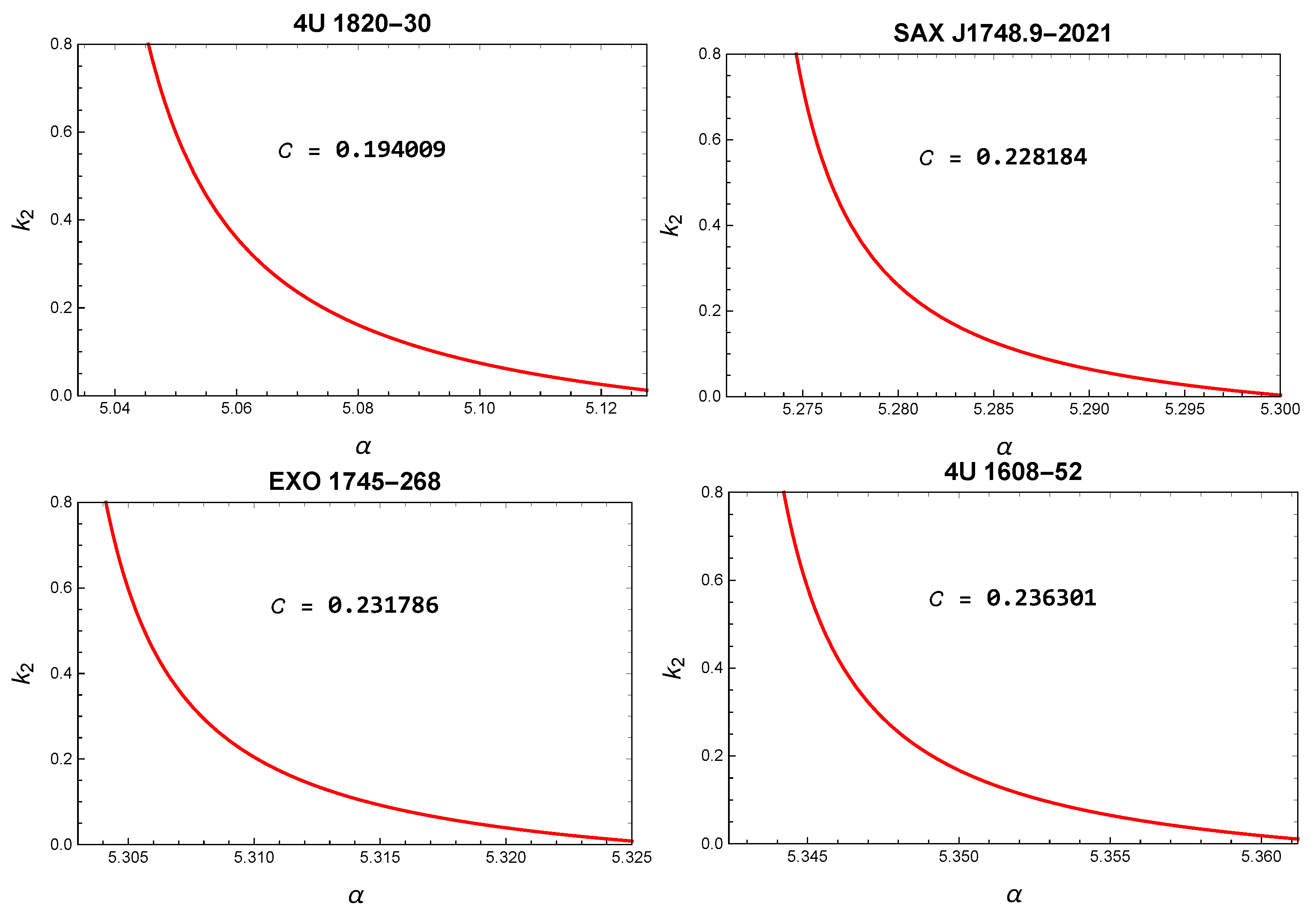
The tidal distortion of NSs in a binary system connects the EOS, describing the nature of the matter composition star with that of the gravitational wave emission during the inspiral [15]. We consider a static spherically symmetric star, immersed in an external quadrupolar tidal field ${\mathcal{E}}_{ij}$ [16,17] arising due to its binary companion. The star in response to the tidal field develops quadrupole moments ${\mathcal{Q}}_{ij}$, which can be related to the linear order external tidal field ${\mathcal{E}}_{ij}$ as [17].

$$\begin{array}{c}\hfill {\mathcal{Q}}_{ij}=-\Lambda {\mathcal{E}}_{ij},\end{array}$$

(1)

where $\Lambda$ is the tidal deformability of the NS and is related to the $l=2$ dimensionless TLN $k_2$ as [17]

$$\begin{array}{c}\hfill k_2={\displaystyle \frac{3}{2}}\Lambda R^{-5}.\end{array}$$

(2)

The background geometry of spacetime of a spherical static star can be written as

$$\begin{array}{cc}\hfill {}^{\left(0\right)}d{s}^2& {=}^{\left(0\right)}{g}_{\mu \nu }d{x}^{\mu }d{x}^{\nu }\hfill \\ & \hfill =-e^{2\nu \left(r\right)}d{t}^2+e^{2\lambda \left(r\right)}d{r}^2+r^2\left(d{\theta }^2+{sin}^2\theta d{\varphi }^2\right).\end{array}$$

(3)

For the spherically static metric (3), the stress-energy tensor is given as

$$\begin{array}{c}\hfill {}^{\left(0\right)}{T}_{\chi }^{\xi }=\left(\rho +p_t\right)u^{\xi }{u}_{\chi }+p_t{g}_{\chi }^{\xi }+\left(p_r-p_t\right){\eta }^{\xi }{\eta }_{\chi },\end{array}$$

(4)

where $u^{\xi }{u}_{\xi }=-1$, ${\eta }^{\xi }{\eta }_{\xi }=1$ and ${\eta }^{\xi }{u}_{\xi }=0$.

We choose a particular model, which is an anisotropic generalization of the Tolman IV Model [18], given as

$$\begin{array}{ccc}\hfill e^{2\nu }& =& A^2(1+aC{r}^2),\hfill \end{array}$$

(5)

$$\begin{array}{ccc}\hfill e^{2\lambda }& =& \frac{1}{\frac{\left(a\mathrm{C}{r}^2+1\right)\left(1-B\mathrm{C}{r}^2\right)}{2a\mathrm{C}{r}^2+1}-\frac{\alpha \mathrm{C}{r}^2}{2a\mathrm{C}{r}^2+1}}.\hfill \end{array}$$

(6)

It is interesting to note that for $\alpha =0$, this solution reduces to the well-known Tolman IV solution [19].

For the line element (3), the independent set of the Einstein field equations are then obtained as

$$\begin{array}{ccc}\hfill 8\pi \rho & =& \frac{1}{r^2}{\left[r(1-e^{-2\lambda })\right]}^{\prime },\hfill \end{array}$$

(7)

$$\begin{array}{ccc}\hfill 8\pi p_r& =& -\frac{1}{r^2}\left(1-e^{-2\lambda }\right)+\frac{2{\nu }^{\prime }}{r}{e}^{-2\lambda },\hfill \end{array}$$

(8)

$$\begin{array}{ccc}\hfill 8\pi p_t& =& e^{-2\lambda }\left({\nu }^{″}+{\nu }^{\prime 2}+\frac{{\nu }^{\prime }}{r}-{\nu }^{\prime }{\lambda }^{\prime }-\frac{{\lambda }^{\prime }}{r}\right),\hfill \end{array}$$

(9)

where primes (${}^{\prime }$) denote differentiation with respect to r. In the field Equations (7)–(9), we have assumed $G=1=c$. The system of equations determines the behaviour of the gravitational field of an anisotropic imperfect fluid sphere.

For the assumed solutions we have

$$\begin{array}{ccc}\hfill 8\pi \rho & =& \frac{C\left(a\left(C{r}^2\left(a\left(6BC{r}^2+2\right)+2\alpha +7B\right)+3\right)+3(\alpha +B)\right)}{{\left(2aC{r}^2+1\right)}^2},\hfill \end{array}$$

(10)

$$\begin{array}{ccc}\hfill 8\pi p_r& =& -\frac{C\left(aC{r}^2+1\right)\left(a\left(3BC{r}^2-1\right)+B\right)+\alpha C\left(3aC{r}^2+1\right)}{\left(aC{r}^2+1\right)\left(2aC{r}^2+1\right)},\hfill \end{array}$$

(11)

$$\begin{array}{ccc}\hfill 8\pi p_t& =& -\frac{C{\left(aC{r}^2+1\right)}^2\left(a\left(3BC{r}^2-1\right)+B\right)+\alpha C\left(aC{r}^2\left(aC{r}^2+3\right)+1\right)}{{\left(aC{r}^2+1\right)}^2\left(2aC{r}^2+1\right)},\hfill \end{array}$$

(12)

$$\begin{array}{ccc}\hfill 8\pi \Delta & =& \frac{a\alpha {\mathrm{C}}^2{r}^2}{{\left(a\mathrm{C}{r}^2+1\right)}^2},\hfill \end{array}$$

(13)

where we define $\Delta =8\pi (p_t-p_r)$ as the measure of anisotropy of the spherical system.

The exterior Schwarzschild metric is

$$d{s}^2=-\left(1-\frac{2M}{r}\right)d{t}^2+{\left(1-\frac{2M}{r}\right)}^{-1}d{r}^2+r^2(d{\theta }^2+{sin}^2\theta d{\varphi }^2),$$

(14)

across the boundary of the star $r=R$, where M is the total mass of the sphere.

Making use of the junction conditions, the constants $A,B,C$ are determined as

$$\begin{array}{ccc}\hfill A& =& \frac{\sqrt{R-3M}}{\sqrt{R}},\hfill \end{array}$$

(15)

$$\begin{array}{ccc}\hfill C& =& \frac{M}{a{R}^3-3aM{R}^2},\hfill \end{array}$$

(16)

$$\begin{array}{ccc}\hfill B& =& \frac{(R-3M)\left(a\right(R-2M)-\alpha R)}{R(R-2M)}.\hfill \end{array}$$

(17)

Now the background metric ${}^{\left(0\right)}{g}_{\mu \nu }\left(x^{\nu }\right)$ under the influence of an external tidal field with a small perturbation $h_{\mu \nu }\left(x^{\nu }\right)$ gets modified as

$$\begin{array}{c}\hfill g_{\mu \nu }\left(x^{\nu }\right){=}^{\left(0\right)}{g}_{\mu \nu }\left(x^{\nu }\right)+h_{\mu \nu }\left(x^{\nu }\right).\end{array}$$

(18)

For the linearized metric perturbation $h_{\mu \nu }$, using the method as in [20,21], without loss of generality, we restrict ourselves to static $l=2,m=0$ even parity perturbation. The perturbed metric, with the assumption that the tidal deformation will be axis symmetric around the line connecting the two stars, which we take as the axis of spherical harmonic decomposition, becomes

$$\begin{array}{c}\hfill h_{\mu \nu }=diag\left[H_0\left(r\right)e^{2\nu },H_2\left(r\right)e^{2\lambda },r^{2}K\left(r\right),r^2{sin}^2\theta K\left(r\right)\right]Y_{2m}(\theta ,\varphi ).\end{array}$$

(19)

Furthermore, the perturbed energy momentum tensor is defined by $T_{\chi }^{\xi }{=}^{\left(0\right)}{T}_{\chi }^{\xi }+\delta T_{\chi }^{\xi }$, where the non-zero components of $T_{\chi }^{\xi }$ are: $\delta T_t^t=-{\displaystyle \frac{d\rho }{d{p}_r}}\delta p_{r}Y(\theta ,\varphi ),\delta T_r^r=\delta p_r\left(r\right)Y(\theta ,\varphi ),$ & $\delta T_{\theta }^{\theta }=\delta T_{\varphi }^{\varphi }=\frac{d{p}_t}{d{p}_r}\delta p_r\left(r\right)Y(\theta ,\varphi )$. With these perturbed quantities, we can write down the perturbed Einstein field equation as follows:

$$\begin{array}{c}\hfill G_{\chi }^{\xi }=8\pi T_{\chi }^{\xi },\end{array}$$

(20)

where the Einstein tensor $G_{\chi }^{\xi }$ is calculated using the metric $g_{\chi \xi }$.

From different components of the background Einstein field equation ${}^{\left(0\right)}{G}_{\chi }^{\xi }=8{\pi }^{\left(0\right)}{T}_{\chi }^{\xi }$, we can have the following relationships:

$$\begin{array}{cc}\hfill {}^{\left(0\right)}{G}_t^t& =8{\pi }^{\left(0\right)}{T}_t^t\Rightarrow {\lambda }^{\prime }\left(r\right)=\frac{8\pi r^2{e}^{2\lambda \left(r\right)}\rho \left(r\right)-e^{2\lambda \left(r\right)}+1}{2r},\hfill \end{array}$$

(21)

$$\begin{array}{cc}\hfill {}^{\left(0\right)}{G}_r^r& =8{\pi }^{\left(0\right)}{T}_r^r\Rightarrow {\nu }^{\prime }\left(r\right)=\frac{8\pi r^2{p}_r\left(r\right)e^{2\lambda \left(r\right)}+e^{2\lambda \left(r\right)}-1}{2r},\hfill \end{array}$$

(22)

where and hereafter the prime denotes the derivative w.r.t. the radial coordinate r.

In addition, we know that ${\nabla }_{\xi }^{\left(0\right)}{T}_{\chi }^{\xi }=0$. Now choosing $\xi =r$, by expanding and solving the equation, we can find the expression

$$\begin{array}{c}\hfill p_r^{\prime }\left(r\right)=\frac{-r{p}_r\left(r\right){\nu }^{\prime }\left(r\right)-2p_r\left(r\right)+2p_t\left(r\right)-r\rho \left(r\right){\nu }^{\prime }\left(r\right)}{r}.\end{array}$$

(23)

Again from the various components of the perturbed Einstein Equation (20), we get the following relations

$$\begin{array}{cc}\hfill & G_{\theta }^{\theta }-G_{\varphi }^{\varphi }=0\Rightarrow H_0\left(r\right)=H_2\left(r\right)=H\left(r\right),\hfill \end{array}$$

(24)

$$\begin{array}{cc}\hfill & G_r^{\theta }=0\Rightarrow K^{\prime }=H^{\prime }+2H{\nu }^{\prime },\hfill \end{array}$$

(25)

$$\begin{array}{cc}\hfill & G_{\theta }^{\theta }+G_{\varphi }^{\varphi }=8\pi (T_{\theta }^{\theta }+T_{\varphi }^{\varphi })\Rightarrow \delta p_r=\frac{H\left(r\right)e^{-2\lambda \left(r\right)}\left({\lambda }^{\prime }\left(r\right)+{\nu }^{\prime }\left(r\right)\right)}{8\pi \frac{d{p}_t}{d{p}_r}r}.\hfill \end{array}$$

(26)

Using the identity

$${\displaystyle \frac{{\partial }^{2}Y(\theta ,\varphi )}{\partial {\theta }^2}}+cot\left(\theta \right){\displaystyle \frac{\partial Y(\theta ,\varphi )}{\partial \theta }}+{csc}^2\left(\theta \right){\displaystyle \frac{{\partial }^{2}Y(\theta ,\varphi )}{\partial {\varphi }^2}}=-6Y(\theta ,\varphi )$$

and Equations (21)–(26), we have the master equation for $H\left(r\right)$ as

$$\begin{array}{cc}\hfill & -\frac{1}{e^{-2\lambda \left(r\right)}Y(\theta ,\varphi )}\left[G_t^t-G_r^r\right]=-\frac{8\pi }{e^{-2\lambda \left(r\right)}Y(\theta ,\varphi )}\left[T_t^t-T_r^r\right]\hfill \\ \hfill & \Rightarrow H^{″}\left(r\right)+\mathcal{R}{H}^{\prime }\left(r\right)+\mathcal{S}H\left(r\right)=0,\hfill \end{array}$$

(27)

where

$$\begin{array}{c}\hfill \mathcal{R}=-\left(\frac{-e^{2\lambda \left(r\right)}-1}{r}-4\pi r{e}^{2\lambda \left(r\right)}(p_r\left(r\right)-\rho \left(r\right))\right),\end{array}$$

(28)

$$\begin{array}{cc}\hfill \mathcal{S}& =-\left(\frac{4e^{2\lambda \left(r\right)}+e^{4\lambda \left(r\right)}+1}{r^2}+64{\pi }^2{r}^2{p}_r{\left(r\right)}^2{e}^{4\lambda \left(r\right)}+16\pi e^{2\lambda \left(r\right)}\left(p_r\left(r\right)\left(e^{2\lambda \left(r\right)}-2\right)\right.\right.\hfill \\ \hfill & \left.\left.-p_t\left(r\right)-\rho \left(r\right)\right)+\frac{-4\pi \frac{d\rho }{d{p}_r}{e}^{2\lambda \left(r\right)}(p_r\left(r\right)+\rho \left(r\right))-4\pi e^{2\lambda \left(r\right)}(p_r\left(r\right)+\rho \left(r\right))}{\frac{d{p}_t}{d{p}_r}}\right).\hfill \end{array}$$

(29)

The vacuum exterior of the star is of Schwarzschild type, so that by setting $\rho =0,p_r=0,p_t=0$ and $e^{2\lambda }=1/(1-2M/r)$, the master Equation (27) becomes

$$\begin{array}{c}\hfill -H^{″}\left(r\right)-\frac{2(M-r)H^{\prime }\left(r\right)}{r(2M-r)}+\frac{2H\left(r\right)\left(2M^2-6Mr+3r^2\right)}{r^2{(r-2M)}^2}=0.\end{array}$$

(30)

The solution to this second order differential Equation (30) is

$$\begin{array}{cc}\hfill H\left(r\right)=& {\displaystyle \frac{1}{2M^{2}r(2M-r)}}\left[c_2\left(-2M\left(2M^3+4M^{2}r-9M{r}^2+3r^3\right)-3r^2{(r-2M)}^2\right.\right.\hfill \\ \hfill & \left.\left.\times log\left(\frac{r}{M}-2\right)+3r^2{(r-2M)}^{2}log\left(\frac{r}{M}\right)\right)\right]+\frac{3c_{1}r(2M-r)}{M^2},\hfill \end{array}$$

(31)

where $c_1$ and $c_2$ are integration constants. In order to obtain the expressions for these constants, we perform a series expansion of Equation (31)

$$\begin{array}{c}\hfill H\left(r\right)=-\frac{3c_1{r}^2}{M^2}+\frac{6c_{1}r}{M}-\frac{c_2\left(8M^3\right)}{5r^3}+\mathcal{O}\left({\left(\frac{1}{r}\right)}^4\right).\end{array}$$

(32)

Now, at large r, the metric coefficient $g_{tt}$ is given by [17]:

$$\begin{array}{cc}\hfill \frac{\left(1-g_{tt}\right)}{2}=& -\frac{M}{r}-\frac{3{\mathcal{Q}}_{ij}}{2r^3}\left(n^i{n}^j-\frac{1}{3}{\delta }^{ij}\right)+\mathcal{O}\left(\frac{1}{r^4}\right)+\frac{1}{2}{\mathcal{E}}_{ij}{x}^i{x}^j+\mathcal{O}\left(r^3\right),\hfill \end{array}$$

(33)

where $n^i=x^i/r$.

Matching the asymptotic solution from Equation (32) with the expansion from Equation (33) and using the Equation (1), we have

$$\begin{array}{c}\hfill c_1=-\frac{M^2\mathcal{E}}{3},c_2=\frac{15\mathcal{Q}}{8M^3}.\end{array}$$

(34)

Using Equations (34), (31) and (2), we obtain the expression for TLN $k_2$ as follows:

$$\begin{array}{c}\hfill k_2=\left[8{(1-2\mathcal{C})}^2{\mathcal{C}}^5(2\mathcal{C}(\mathit{y}-1)-\mathit{y}+2)\right]/X,\end{array}$$

(35)

where

$$\begin{array}{cc}\hfill X& =\left(5\right(2\mathcal{C}\left(\mathcal{C}\right(2\mathcal{C}\left(\mathcal{C}\right(2\mathcal{C}(\mathit{y}+1)+3\mathit{y}-2)-11\mathit{y}+13)+3(5\mathit{y}-8))-3\mathit{y}+6)\hfill \\ \hfill & \left.\left.+3{(1-2\mathcal{C})}^2(2\mathcal{C}(\mathit{y}-1)-\mathit{y}+2)log\left(\frac{1}{\mathcal{C}}-2\right)-3{(1-2\mathcal{C})}^2(2\mathcal{C}(\mathit{y}-1)-\mathit{y}+2)log\left(\frac{1}{\mathcal{C}}\right)\right)\right).\hfill \end{array}$$

(36)

Here, the compactness $\mathcal{C}=\frac{M}{R}$ and $\mathit{y}$ depend on $r,H$ and its derivatives evaluated at R with

$$\begin{array}{c}\hfill {\left.\mathit{y}={\displaystyle \frac{r{H}^{\prime }\left(r\right)}{H\left(r\right)}}\right|}_{r=R}.\end{array}$$

(37)

To calculate numerically the value of $k_2$ for a particular NS [22], one needs to modify the master Equation (27) using Equation (37) as

$$\begin{array}{c}\hfill r{y}^{\prime }+y^2+(r\mathcal{R}-1)y+r^2\mathcal{S}=0.\end{array}$$

(38)

3. Results

The recent data available from the pulsar $4U1608-52$ (for the star to be composed of an anisotropic fluid distribution with $\alpha =0.5$), whose estimated mass and radius are $M=1.57M_{\odot }$ and $R=9.8km$, respectively [23,24], are used to find the constants are calculated as $A=0.53953,B=0.291097,C=0.008452$. We set $a=1$. Making use of these values, we show the nature of all the physically meaningful quantities graphically in Figure 1.

Using the initial condition $y\left(0\right)=2$ and all the mentioned equations, Equation (38) for a particular NS, can be numerically calculated. Having the numerical value of y, for a particular NS, from Equation (35), the TLN $k_2$ can be obtained numerically.

4. Conclusions

The plots clearly show that all the quantities comply with the requirements of a physically viable realistic star. In particular, the figures highlight the effect of anisotropy on the gross physical behaviour of the compact star. In Figure 2, the TLN $k_2$ is plotted against $\alpha$ for different compact objects with compactness $\mathcal{C}$. From this panel of figures, we note that $k_2$ decreases monotonically with increasing $\alpha$. This is a much expected physical property of a compact object with anisotropy.

References

1. Abbott, B.P.; Abbott, R.; Abbott, T.D.; Acernese, F.; Ackley, K.; Adams, C.; Cahillane, C. GW170817: Observation of gravitational waves from a binary neutron star inspiral. Phys. Rev. Lett. 2017, 119, 161101. [Google Scholar] [CrossRef] [Green Version]
2. Sawyer, R.F. Condensed π- phase in neutron-star matter. Phys. Rev. Lett. 1972, 29, 382–385. [Google Scholar] [CrossRef]
3. Takatsuka, T.; Tamagaki, R. Nucleon superfluidity in kaon-condensed neutron stars. Prog. Theor. Phys. 1995, 94, 457–461. [Google Scholar] [CrossRef]
4. Kippenhahn, R.; Weigert, A. Stellar Structure and Evolution; Springer: Berlin, Germany, 1990. [Google Scholar]
5. Ruderman, R. Pulsars: Structures and dynamics. Ann. Rev. Astron. Astrophys. 1972, 10, 427–476. [Google Scholar] [CrossRef]
6. Weber, F. Pulsars as Astrophysical Observatories for Nuclear and Particle Physics; IOP Publishing: Bristol, UK, 1999. [Google Scholar]
7. Sokolov, A.I. Phase transformations in a superfluid neutron liquid. J. Exp. Theor. Phys. 1980, 79, 1137–1140. [Google Scholar]
8. Mak, M.K.; Harko, T. An exact anisotropic quark star model. Chin. J. Astron. Astrophys. 2002, 2, 248–269. [Google Scholar] [CrossRef]
9. Mak, M.K.; Harko, T. Anisotropic stars in general relativity. Proc. R. Soc. Lond. Ser. A 2003, 459, 393–408. [Google Scholar] [CrossRef] [Green Version]
10. Ivanov, B.V. Maximum bounds on the surface redshift of anisotropic stars. Phys. Rev. D 2002, 65, 104011. [Google Scholar] [CrossRef] [Green Version]
11. Gleiser, M.; Dev, K. Anistropic stars: Exact solutions and stability. Int. J. Mod. Phys. D 2004, 13, 1389–1397. [Google Scholar] [CrossRef]
12. Böhmer, C.G.; Harko, T. Bounds on the basic physical parameters for anisotropic compact general relativistic objects. Class. Quantum Gravit. 2006, 23, 6479–6491. [Google Scholar] [CrossRef] [Green Version]
13. Bayin, S.S. Anisotropic fluid spheres in general relativity. Phys. Rev. D 1982, 26, 1262–1274. [Google Scholar] [CrossRef]
14. Herrera, L.; Santos, N.O. Local anisotropy in self-gravitating systems. Phys. Rep. 1997, 286, 53–130. [Google Scholar] [CrossRef]
15. Hinderer, T.; Lackey, B.D.; Lang, R.N.; Read, J.S. Tidal deformability of neutron stars with realistic equations of state and their gravitational wave signatures in binary inspiral. Phys. Rev. D 2010, 81, 123016. [Google Scholar] [CrossRef] [Green Version]
16. Flanagan, E.E.; Hinderer, T. Constraining neutron-star tidal Love numbers with gravitational-wave detectors. Phys. Rev. D 2008, 77, 021502. [Google Scholar] [CrossRef] [Green Version]
17. Hinderer, T. Tidal Love Numbers of neutron stars. Astrophys. J. 2008, 677, 1216–1220. [Google Scholar] [CrossRef]
18. Thirukkanesh, S.; Ragel, F.C.; Sharma, R.; Das, S. Anisotropic generalization of well-known solutions describing relativistic self-gravitating fluid systems: An algorithm. Eur. Phys. J. C 2018, 78, 31. [Google Scholar] [CrossRef] [Green Version]
19. Tolman, R.C. Static solutions of Einstein’s field equations for spheres of fluid. Phys. Rev. 1939, 55, 364–373. [Google Scholar] [CrossRef] [Green Version]
20. Regge, T.; Wheeler, J.A. Stability of a Schwarzschild Singularity. Phys. Rev. D 1957, 108, 1063–1069. [Google Scholar] [CrossRef]
21. Biswas, B.; Bose, S. Tidal deformability of an anisotropic compact star: Implications of GW170817. Phys. Rev. D 2019, 99, 104002. [Google Scholar] [CrossRef] [Green Version]
22. Rahmansyah, A.; Sulaksono, A.; Wahidin, A.B.; Setiawan, A.M. Anisotropic neutron stars with hyperons: Implication of the recent nuclear matter data and observations of neutron stars. Eur. Phys. J. C 2020, 80, 769. [Google Scholar] [CrossRef]
23. Roupas, Z.; Nashed, G.G. Anisotropic neutron stars modelling: Constraints in Krori–Barua spacetime. Eur. Phys. J. C 2020, 80, 905. [Google Scholar] [CrossRef]
24. Özel, F.; Psaltis, D.; Güver, T.; Baym, G.; Heinke, C.; Guillot, S. The dense matter equation of state from neutron star radius and mass measurements. ApJ 2016, 820, 28. [Google Scholar] [CrossRef]
Figure 1. Physical features are plotted against the radial parameter for the compact star 4U 1608-52.
Psf 02 00029 g001
Figure 2. k 2 is plotted against α for different compact objects with compactness C only for the allowed values of α .
Psf 02 00029 g002
Publisher’s Note: MDPI stays neutral with regard to jurisdictional claims in published maps and institutional affiliations.