Casimir Effect as a Probe for New Physics Phenomenology ^†

Abstract

We show some recent cutting-edge results associated with the Casimir effect. Specifically, we focused our attention on the remarkable sensitivity of the Casimir effect to new physics phenomenology. Such an awareness can be readily discerned by virtue of the existence of extra contributions that the measurable quantities (such as the emergent pressure and strength within the experimental apparatus) acquire for a given physical setting. In particular, by relying on the above framework, we outlined the possibility of detecting the predictions of a novel quantum field theoretical description for particle mixing according to which the flavor and the mass vacuum are unitarily non-equivalent. Furthermore, by extending the very same formalism to curved backgrounds, the opportunity to probe extended models of gravity that encompass local Lorentz symmetry breaking and the strong equivalence principle violation was also discussed. Finally, the influence of quantum gravity on the Casimir effect was briefly tackled by means of heuristic considerations. In a similar scenario, the presence of a minimal length at the Planck scale was the source of the discrepancy with the standard outcomes.

1. Introduction

Undoubtedly, the Casimir effect can be deemed as the first-ever manifestation of zero-point energy, and it arises any time a quantum field is confined in a small region of space [1,2,3]. The confinement gives rise to a net attractive force between the binding objects, the intensity of which depends not only on the geometry of the volume in which the field is bound, but also on its nature (i.e., scalar, fermion, etc.) and on the spacetime in which the experiment takes place. Initially computed as the result of molecular van der Waals forces, after Bohr’s suggestion, the Casimir effect was derived by relying on quantum field theoretical considerations only, thus showing how the two different interpretations are but two sides of the same coin [3]. However, due to the smallness of the generated force, it took a long time before its first experimental verification [4], and since then, many efforts have been deployed to acquire new data more accurately.

In this paper, we summarized several recent outcomes related to the Casimir effect that may help to unravel new physics phenomenology, in the context of both particle physics and gravitation. To this aim, we first reviewed an important achievement associated with particle mixing, thus showing how we can discriminate the true physical vacuum among the unitarily nonequivalent ones connected with a mixed field [5]. After that, we focused our attention on the gravitational domain to investigate the sensitivity of the Casimir effect to the presence of extended theories of gravity. Finally, we analyzed the regime where quantum and gravitational influences coexist and allow for the existence of a minimal length at the Planck scale, as firstly predicted in the framework of string theory [6,7,8,9].

Throughout the work, we use natural units $\hslash =c=1$.

2. Results

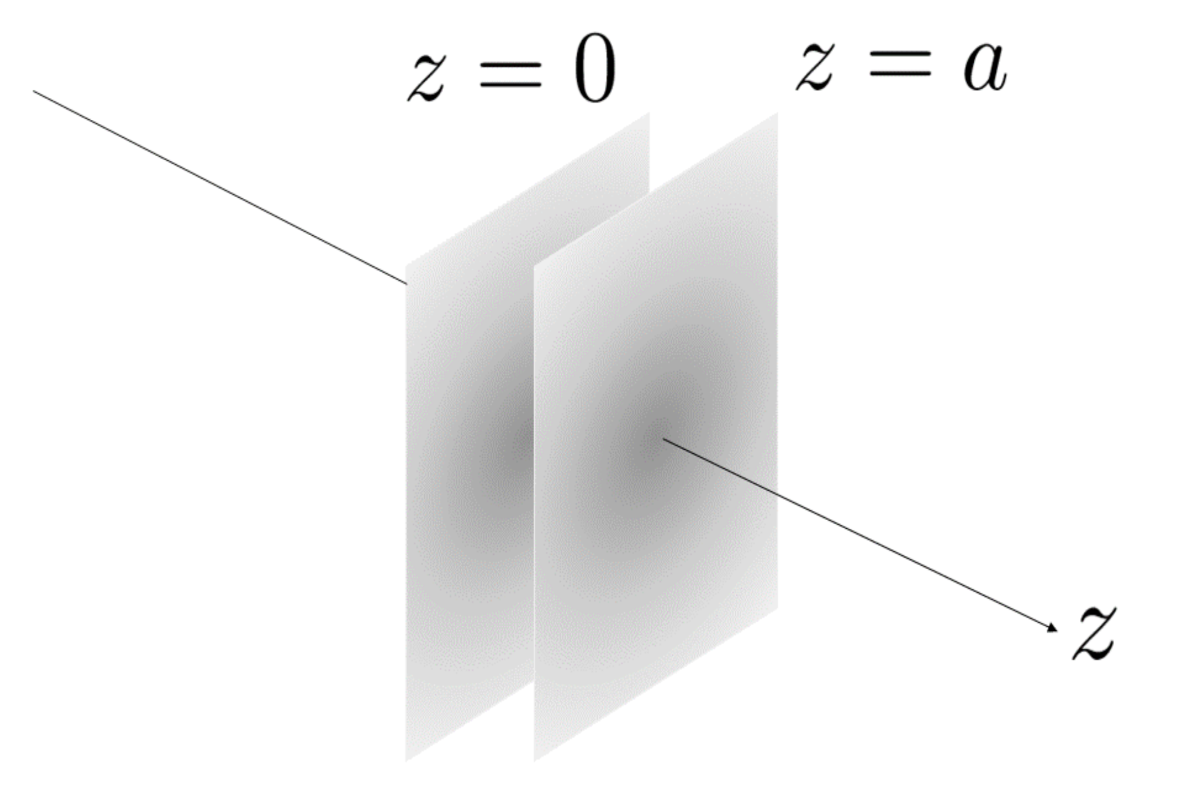
In this section, we thoroughly address all the points that were introduced above. Without delving into the technical details, we provide the general description, as well as the desired result. Before that, however, we briefly sketch how to compute the Casimir effect as done in [3]. For this purpose, consider a massless scalar field that is confined between two thin plates with relative distance a as in Figure 1.

Since the field is not present on the plates, we require the following Dirichlet boundary condition for the field modes:

$$\varphi (t,{\mathbf{x}}_{\perp },0)=\varphi (t,{\mathbf{x}}_{\perp },a)=0.$$

(1)

At this point, one can evaluate the vacuum energy per unit transverse area:

$$\epsilon =\langle 0\left|T_{00}\right|0\rangle =\frac{1}{2}\sum _n\int \frac{d^2{k}_{\perp }}{{\left(2\pi \right)}^2}\sqrt{k_{\perp }^2+\frac{n^2{\pi }^2}{a^2}},$$

(2)

where $T_{00}$ is the 00-th component of the stress–energy tensor. The previous equation can be solved via dimensional regularization [3] and yields:

$$\epsilon =-\frac{{\pi }^2}{1440}\frac{1}{a^3}.$$

(3)

The physical quantity of the Casimir experiment is the attractive pressure that stems from the confinement of the field or, in other words, from the gap between the modes outside the plates (continuous) and the inner ones (discrete). To evaluate the force per unit area, we observe that it is given by $P=-\partial \epsilon /\partial a$, and hence:

$$P=-\frac{{\pi }^2}{480}\frac{1}{a^4}.$$

(4)

The reasoning carried out so far is employed in all the upcoming discussions, the only difference being the physical setting.

2.1. Casimir Effect and Particle Mixing

To simplify the following treatment, we work in $1+1$ dimensions and with a scalar mixed field having two flavors only (with the word flavor, here, we refer to a given mixed quantum number; as a matter of fact, flavor is typically used only for neutrinos and not for mixed mesons). Under these circumstances, we can resort to an already existing calculation in the literature regarding the attractive Casimir strength due to a massive scalar field in $1+1$ dimensions, namely [10]:

$$F=-\frac{m^2}{\pi }\sum _n\left[K_2\left(2amn\right)-\frac{K_1\left(2amn\right)}{2amn}\right],$$

(5)

where a is the displacement between the plates, m the mass of the field, and $K_{\nu }\left(x\right)$ the modified Bessel function of the second kind.

Starting from the previous premise, a massive scalar mixed field can be investigated, whose Lagrangian in the flavor and mass basis reads: -4.6cm0cm

$$\mathcal{L}=\sum _{\sigma =A,B}\left({\partial }_{\mu }{\varphi }_{\sigma }^{†}{\partial }^{\mu }{\varphi }_{\sigma }-m_{\sigma }^2{\varphi }_{\sigma }^{†}{\varphi }_{\sigma }\right)-m_{AB}^2\left({\varphi }_A^{†}{\varphi }_B+{\varphi }_B^{†}{\varphi }_A\right)=\sum _{i=1,2}\left({\partial }_{\mu }{\varphi }_i^{†}{\partial }^{\mu }{\varphi }_i-m_i^2{\varphi }_i^{†}{\varphi }_i\right),$$

(6)

where in the first part, $\sigma$ labels the flavor and the mass matrix is clearly nondiagonal. To make it diagonal as in the second part of Equation (6), we have to introduce a unitary matrix U, which can also be used to switch between the flavor and the mass basis, i.e., ${\varphi }_f=U{\varphi }_m$. In the latter representation, the Lagrangian (6) is simply the sum of two noninteracting scalar fields.

At the level of the vacuum states, the above mixing implies that, in the infinite volume limit, the flavor and the mass Fock spaces become unitarily nonequivalent [11]:

$$\underset{V\to \infty }{lim}{}_{AB}{\langle 0|0\rangle }_{12}=0,$$

(7)

and the flavor vacuum must be viewed as a condensate of mass field excitations. Therefore, the choice of the correct vacuum is crucial for the Casimir effect, and in light of the previous observations, we know that its phenomenology can be deemed as an invaluable probe to check which of the two vacua is more fundamental [12]. Indeed, starting from the mass vacuum, we would obtain:

$$F_m=-\sum _{j=1,2}\frac{m_j^2}{\pi }\sum _n\left[K_2\left(2a{m}_{j}n\right)-\frac{K_1\left(2a{m}_{j}n\right)}{2a{m}_{j}n}\right],$$

(8)

whereas by selecting the flavor vacuum and assuming the condition $\delta m^2{a}^2\ll 1$ with $\delta m^2=m_2^2-m_1^2$, we would obtain:

$$F_f=F_m-\frac{3a^2{sin}^2\theta \zeta \left(3\right){\left(\delta m^2\right)}^2}{2{\pi }^3},$$

(9)

where $\zeta \left(x\right)$ is the Riemann zeta function.

2.2. Casimir Effect and Extended Theories of Gravity

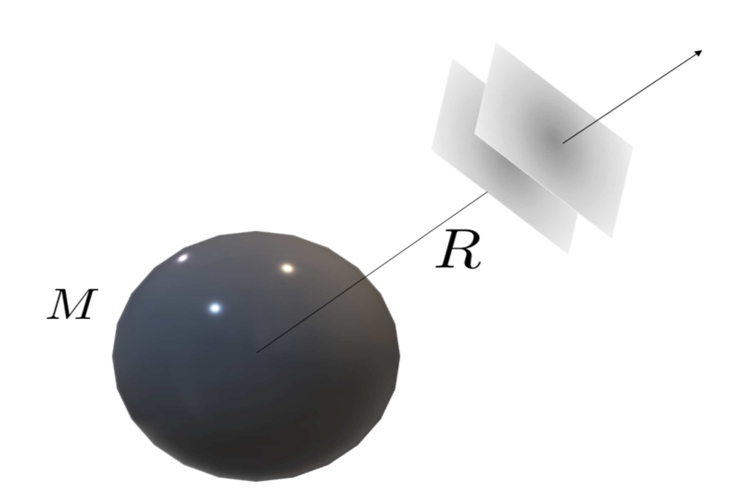
By going back to $3+1$ dimensions and with a single massless scalar field, we can now see what happens when the Casimir apparatus is embedded in a weak gravitational field generated by a source with mass M. The physical setup is shown in Figure 2; in the picture, R denotes the radial distance between the source and the nearer plate, and the radial axis passes through the surface perpendicularly.

Should we perform the investigation in the weak-field limit of the Schwarzschild solution in isotropic coordinates, that is:

$$g_{00}=1+2{\varphi }_{GR},g_{ij}=-\left(1-2{\varphi }_{GR}\right){\delta }_{ij},$$

(10)

where ${\varphi }_{GR}$ is the usual Newtonian potential, we would end up with a final pressure given by:

$$P=P_0+P_{GR},P_{GR}=-\frac{2{\varphi }_{GR}{a}_P}{3R}{P}_0,$$

(11)

with $P_0$ being the pressure evaluated in the flat case (4) and $a_P$ the proper displacement between the plates.

On the other hand, if we want to work in the context of an extended model of gravity, in general, we have to start from an ensuing gravitational action represented by the usual Einstein–Hilbert contribution together with higher terms in the curvature invariants and with higher derivatives as well, i.e., -4.6cm0cm

$${\displaystyle S=\frac{1}{2{\kappa }^2}\int d^{4}x\sqrt{-g}\left\{\mathcal{R}+\mathcal{F}({\mathcal{R}}^n,{\mathcal{R}}_{\mu \nu }{\mathcal{R}}^{\mu \nu },{\mathcal{R}}_{\mu \nu \rho \lambda }{\mathcal{R}}^{\mu \nu \rho \lambda },\mathcal{R}{\nabla }^{\rho }{\nabla }_{\rho }\mathcal{R},{\mathcal{R}}_{\mu \nu }{\nabla }^{\rho }{\nabla }_{\rho }{\mathcal{R}}^{\mu \nu },\cdots )\right\}.}$$

(12)

In this framework, we note that the general form in which the linearized metric tensor in isotropic coordinates can be cast is [13]:

$$g_{00}=1+2\Phi =1+2{\varphi }_{GR}+2{\varphi }_{ETG},g_{ij}=-\left(1-2\Psi \right){\delta }_{ij}=-\left(1-2{\varphi }_{GR}-2{\psi }_{ETG}\right){\delta }_{ij},$$

(13)

with ${\varphi }_{ETG}$ and ${\psi }_{ETG}$ being the corrections to the Newtonian potential that can be either equal or different.

According to this scenario, the expression for the pressure becomes:

$${\displaystyle P=P_0+P_{GR}+P_{ETG},P_{ETG}=\left[3\left({\varphi }_{ETG}^{\left(0\right)}-{\psi }_{ETG}^{\left(0\right)}\right)-\frac{2}{3}\left(2{\psi }_{ETG}^{\left(1\right)}-{\varphi }_{ETG}^{\left(1\right)}\right)a_P\right]P_0,}$$

(14)

with the notation:

$$f^{\left(0\right)}\left(r\right)=f\left(r\right){|}_{r=R},f^{\left(1\right)}\left(r\right)=\frac{df}{dr}{|}_{r=R}.$$

(15)

This formalism has been employed for several extended models of gravity, among which it is worth recalling quadratic theories of gravity [13] (where it is possible to identify a term related to the strong equivalence principle violation) and the gravitational sector of the Standard Model Extension [14] (which is intimately connected with the local Lorentz violation).

2.3. Casimir Effect and Quantum Gravity

As a final example, we focus on quantum gravitational implications that can be probed via the Casimir effect. Specifically, our attention is devoted to the modification of the usual Heisenberg uncertainty principle:

$$\delta x\delta p\ge \frac{1}{2},$$

(16)

that accounts for the existence of a minimal length at the Planck scale. A similar prediction stems from superstring collisions at high energies [6], but it is also encountered in different frameworks. In a nutshell, the novelty brought forward with respect to Equation (16) is the introduction of a momentum-dependent additive term that goes as:

$$\delta x\ge \frac{1}{2\delta p}+\beta \frac{\delta p}{m_p^2},$$

(17)

where $m_p$ is the Planck mass and $\beta$ is the so-called deformation parameter, which is assumed to be of order unity. It is worth stressing that a similar generalization allows for a brand-new phenomenology in the quantum realm, as the representation of the position and momentum operators has to be modified as well. This can be checked by observing that Equation (17) entails a change in the canonical commutator [15], which is:

$$\left[x,p\right]=i\left[1+\beta {\left(\frac{p}{m_p}\right)}^2\right].$$

(18)

Concerning the Casimir effect, one can then show [16] that the qualitative behavior of the energy per unit surface (3) as a function of a can be straightforwardly deduced from the uncertainty relations by means of heuristic considerations only. More precisely, the arising attractive force can be explained in terms of an imbalance of virtual photons popping out from the vacuum between the region inside the plates and the external space. Therefore, the Casimir pressure can actually be regarded as a “radiative” pressure, and on average, from the (wider) outer region, more photons will hit the plates, thus allowing them come closer. The exact numerical value exhibited in Equation (3) can be reached by requiring that no photon participates in the aforementioned process beyond a certain distance from the plates. A similar reasoning is motivated by the fact that the lifetime of such particles is strictly related to their energy, i.e., $\delta t\simeq 1/\delta E$, which means that highly energetic photons do not live long enough to contribute to the pressure.

The same considerations can be carried out by resorting to the generalized uncertainty principle (17), and qualitatively, we observe that [17,18]:

$${\epsilon }_{HUP}\simeq \frac{1}{a^3},{\epsilon }_{GUP}\simeq \frac{1}{a^3}\left[1+\frac{\beta }{a{E}_p}\right],$$

(19)

with $E_p$ being the Planck energy. Although the correction might be irrelevant, by approaching smaller and smaller scales, it can be comparable with the zeroth-order term, thereby plausibly permitting its experimental evidence.

3. Discussion

With this manuscript, we hope to have conveyed the idea that the Casimir effect can safely be viewed as one of the most important experimental tools we have at our disposal to test new physics phenomenology. The results derived here were associated with a massless scalar field, which was but a mere toy model. A more realistic analysis would instead involve fermion and vector fields, but this aspect is still under active investigation. Nevertheless, in conjunction with the aforesaid developments and taking into account the accurate geometries realized in laboratories, an improvement of the apparatus sensitivity may potentially open the door to the detection of physical phenomena beyond the Standard Model and General Relativity by relying on the Casimir effect.

References

- Casimir, H.B.G. On the Attraction Between Two Perfectly Conducting Plates. Indag. Math. 1948, 10, 261. [Google Scholar]
- Casimir, H.B.G.; Polder, D. The Influence of retardation on the London-van der Waals forces. Phys. Rev. D 1948, 73, 360. [Google Scholar] [CrossRef]
- Milton, K.A. The Casimir Effect: Physical Manifestations of Zero Point Energy; World Scientific Publishing Company: Singapore, 2001. [Google Scholar]
- Lamoreaux, S.K. Demonstration of the Casimir force in the 0.6 to 6 micrometers range. Phys. Rev. Lett. 1997, 78, 5. [Google Scholar] [CrossRef] [Green Version]
- Blasone, M.; Vitiello, G. Quantum field theory of fermion mixing. Ann. Phys. 1995, 244, 283. [Google Scholar] [CrossRef] [Green Version]
- Amati, D.; Ciafaloni, M.; Veneziano, G. Superstring Collisions at Planckian Energies. Phys. Lett. B 1987, 197, 81. [Google Scholar] [CrossRef] [Green Version]
- Gross, D.J.; Mende, P.E. The High-Energy Behavior of String Scattering Amplitudes. Phys. Lett. B 1987, 197, 129. [Google Scholar]
- Konishi, K.; Paffuti, G.; Provero, P. Minimum Physical Length and the Generalized Uncertainty Principle in String Theory. Phys. Lett. B 1990, 234, 276. [Google Scholar]
- Maggiore, M. A Generalized uncertainty principle in quantum gravity. Phys. Lett. B 1993, 304, 65. [Google Scholar]
- Mobassem, S. Casimir effect for massive scalar field. Mod. Phys. Lett. A 2014, 29, 1450160. [Google Scholar] [CrossRef]
- Blasone, M.; Capolupo, A.; Romei, O.; Vitiello, G. Quantum field theory of boson mixing. Phys. Rev. D 2001, 63, 125015. [Google Scholar] [CrossRef] [Green Version]
- Blasone, M.; Luciano, G.G.; Petruzziello, L.; Smaldone, L. Casimir effect for mixed fields. Phys. Lett. B 2018, 786, 278. [Google Scholar] [CrossRef]
- Buoninfante, L.; Lambiase, G.; Petruzziello, L.; Stabile, A. Casimir effect in quadratic theories of gravity. Eur. Phys. J. C 2019, 79, 41. [Google Scholar] [CrossRef] [PubMed]
- Blasone, M.; Lambiase, G.; Petruzziello, L.; Stabile, A. Casimir effect in Post-Newtonian Gravity with Lorentz-violation. Eur. Phys. J. C 2018, 78, 976. [Google Scholar] [CrossRef]
- Kempf, A.; Mangano, G.; Mann, R.B. Hilbert space representation of the minimal length uncertainty relation. Phys. Rev. D 1995, 52, 1108. [Google Scholar] [CrossRef] [PubMed] [Green Version]
- Giné, J. Casimir effect and the uncertainty principle. Mod. Phys. Lett. A 2018, 33, 1850140. [Google Scholar] [CrossRef]
- Blasone, M.; Lambiase, G.; Luciano, G.G.; Petruzziello, L.; Scardigli, F. Heuristic derivation of the Casimir effect from Generalized Uncertainty Principle. J. Phys. Conf. Ser. 2019, 1275, 012024. [Google Scholar] [CrossRef]
- Blasone, M.; Lambiase, G.; Luciano, G.G.; Petruzziello, L.; Scardigli, F. Heuristic derivation of Casimir effect in minimal length theories. Int. J. Mod. Phys. D 2020, 29, 2050011. [Google Scholar]
Figure 1.
In this figure, the Casimir apparatus is displayed.
Figure 2.
In this figure, the Casimir apparatus in curved spacetime is exhibited.
Publisher’s Note: MDPI stays neutral with regard to jurisdictional claims in published maps and institutional affiliations. |
© 2021 by the author. Licensee MDPI, Basel, Switzerland. This article is an open access article distributed under the terms and conditions of the Creative Commons Attribution (CC BY) license (https://creativecommons.org/licenses/by/4.0/).
Share and Cite
MDPI and ACS Style
Petruzziello, L. Casimir Effect as a Probe for New Physics Phenomenology. Phys. Sci. Forum 2021, 2, 17. https://doi.org/10.3390/ECU2021-09307
AMA Style
Petruzziello L. Casimir Effect as a Probe for New Physics Phenomenology. Physical Sciences Forum. 2021; 2(1):17. https://doi.org/10.3390/ECU2021-09307
Chicago/Turabian StylePetruzziello, Luciano. 2021. "Casimir Effect as a Probe for New Physics Phenomenology" Physical Sciences Forum 2, no. 1: 17. https://doi.org/10.3390/ECU2021-09307