
Two Sets of Boundary Conditions in Cyclical Systems with Goodwill in Capitalization


Lehtoi Research, 81235 Lehtoi, Finland
Foundations 2024, 4(1), 3-13; https://doi.org/10.3390/foundations4010002
Submission received: 25 August 2023
/
Revised: 11 December 2023
/
Accepted: 18 December 2023
/
Published: 20 December 2023
Abstract
:Mathematical analysis is conducted on cyclical systems with goodwill in capitalization. Proportional goodwill vanishes with vanishing tangible value. Correspondingly, periodic boundary condition does not enable commercial utilization of the goodwill. Abandoning the periodic boundary condition enables commercial utilization of the goodwill. Even if a physical system is periodic, an agent can abandon the corresponding boundary condition by divesting. Example cases are shown in terms of boreal forestry systems.
1. Introduction
Intangible assets refer to knowledge, reputation, customer relations, as well as expectations of future events [1,2,3,4]. A goodwill value refers to intangible firm value in excess of the fair market value of its tangible and financial assets [5,6,7]. In terms of accounting, the goodwill value can be exactly determined in the context of a merger or an acquisition, as the distinction between the acquisition price and the book value of tangible and financial assets [6,7]. In the absence of a realized acquisition, the goodwill value is not exactly known—however, it can be approximated based on observations of realized contracts of similar character.
Even if accounting literature discusses goodwill in the context of firm acquisitions, the concept obviously is useful in the valuation of assets other than complete firms. Production resources like machinery or factories may include not only tangible but also intangible value, as well as separate businesses, operative units, or estates. In the case of productive systems, one source of intangible value is the expectation of the value of future production, but others exist [8,9,10,11].
This paper will discuss cyclical productive systems that possibly obey periodic boundary conditions in time. Some systems are inherently periodic: businesses operating according to seasons, such as agricultural systems, fisheries, and even tourism. The periods do not need to be regulated by annual seasons: periods may correspond to rotations in the business of growing multiannual plants [12,13].
While discussing periodic systems, it is stated that the periodic boundary condition can be possibly abandoned. The abandonment of periodic boundary conditions is discussed in the literature [14,15,16], but not with any apparent relation to economic or financial applications. In economics, boundary value problems are often studied, but apparently without reference to periodic boundary conditions [17,18,19].
One straightforward way for an agent to abandon the periodic boundary condition is to divest the periodic business. The main research question here is, what happens to goodwill values under the periodic boundary condition, and how the abandonment of such boundary condition possibly changes the finances.
First, we will present a mathematical analysis of cyclical systems with goodwill value and investigate the effect of periodic boundary conditions on the finances of such systems. Then, results are illustrated with a comprehensive set of case studies, regarding boreal forestry systems.
2. Mathematical Analysis
Let us discuss a cyclical, periodic production system of value V and period duration τ. The periodic boundary condition implies that the value change over one full period results in zero, or
A consequence of the periodic boundary condition in Equation (1) is that within a complete cycle, eventual cumulative value production within the system must be equal to the cumulative extraction of value from the system. The rate of tangible value production is denoted as , and the rate of value extraction (or the rate of distributed dividends) is denoted as . Then,
As corresponds to the production rate of tangible value, the total value V can be divided into a tangible component T and a non-tangible goodwill value D. The periodic boundary condition requires Equation (1) to be satisfied separately for the tangible and the intangible value component. Then,
The expected value of the value extraction rate (or the rate of distributed dividends) is, by definition,
where a refers to the development stage (or age) within the period, and p(a) refers to the probability density of the ages. The expected value of the capitalization is
As a combination of Equations (4) and (5), the expected value of the return rate on capital is
where vanishes due to Equation (1).
As the intangible goodwill D can be merchandized only by divesting a tangible asset, the magnitude of the goodwill must somehow depend on the state of the asset. This can be most simply addressed by assuming that the intangible goodwill D is proportional to the tangible value T through a constant u, or V = T(1 + u). Then,
Equation (7) contains a remarkable result. In the presence of the periodic boundary condition, the appearance of intangible goodwill dilutes the return rate on capital. This is due to the summing of the goodwill change rate into zero in Equation (3). Correspondingly, goodwill values do not appear in the numerator of Equation (7).
It is then worth asking, is it possible to abandon the periodic boundary condition?
That may be possible. The periodic boundary condition becomes abandoned if the asset is divested before the period becomes completed. Then, the starting point of the integration cannot be chosen arbitrarily, as was performed in Equations (1)–(3), and the integration must not extend over a complete period. Consequently, the accumulated intangible goodwill value does not vanish as it did in Equation (3). The expected value of the return rate on capital becomes
A comparison of Equation (8) with Equation (7) reveals some dramatic results. One readily finds that if , Equation (8) coincides with Equation (7). However, if the rate of distributed dividends vanishes, Equation (8) scales the result of Equation (7) by a factor (1 + u). In other words, the return rate on capital is increased by a factor corresponding to the proportion of the intangible goodwill value. This is, however, only a first-order approximation since the expected tangible value depends on the schedules of value growth rate and dividend distribution rate.
On the other hand, if the rate of distributed dividends does not vanish, it reduces the expected value of gain in the numerator of Equation (8). A first-order effect of this would reduce the rate of return on capital. Again, one must consider that distributed dividends within the time frame appearing in Equation (8) do contribute to the expected value of the tangible capitalization appearing in the denominator. Correspondingly, the total effect of eventual intermediate distributed dividends cannot be concluded without detailed knowledge of the process.
3. Example Data
Boreal forestry is adopted as an example of a cyclical productive system with intangible goodwill values. As the justification of the existence of goodwill value includes an expectation of future gains, liquidity aspects, as well as psychological factors [8,9,10,11], observations have indicated that the goodwill value is approximately linearly proportional to the value of tangible assets [20].
Sixteen different sets of initial conditions, regarding boreal forestry, are used to implement the above theoretical results. The sets of initial conditions originate from two different datasets, described in five earlier investigations [20,21,22,23,24]. Briefly, the datasets are described as follows.
Firstly, seven wooded, commercially unthinned stands in Vihtari, eastern Finland, were observed at the age of 30 to 45 years. Secondly, a group of nine setups was created, containing three tree species and three initial sapling densities [23]. The latter approach allowed an investigation of a wide range of stand densities, as well as a comprehensive description of the application of three tree species. The exact initial conditions equal the ones recommended in [23], appearing there in Figures 8 and 9.
The periodic and non-periodic boundary conditions discussed above are applied to both datasets. A proportional goodwill (1 + u) = (1 + 1/2) is applied in Equations (7) and (8). The inflation factor is somewhat arbitrary, but it is based on recent observations [25,26,27], including very recent observations by the author: large, productive forest estates appear to change owners at 150% of the fair forestry value determined by professionals.
Technically, the application of the datasets is the following. Any of the 16 initial conditions, monetized as described in references [20,21,22,23,24], is written in a computer program. Then, a time evolution from any initial condition is established according to the growth model [28], in terms of 30-month timesteps. In the absence of thinnings, this procedure results in an expected value of capital return rate for any rotation age τ, according to Equations (7) and (8), observable at the end of any time step. The rotation age giving the greatest expected value of the capital return rate appears the most feasible, in the absence of thinnings. Then, one thinning is introduced, experimenting with its timing, severity, allocation to tree species, and diameter classes, within the computer program. If the thinning is successful in improving the maximal expected value of the capital return rate, it is considered feasible. If thinning succeeds in improving the expected value of the capital return rate, another thinning is introduced, which again experiments with timing, severity, and allocation in terms of both introduced thinnings. Further thinnings are introduced this way, one by one, provided that the previous one is successful in improving the expected value of the capital return rate. It is worth noting that in principle, two or more thinnings could be financially feasible even if a single commercial thinning would not be profitable. However, the author is not aware of any such occurrence in boreal forestry, where the number of thinnings tends to be limited because of the requirements of operational efficiency.
Within these example cases, under the two sets of boundary conditions, two forestry strategies are referred to. Firstly, the periodic boundary condition of Equation (1) is accepted. Consequently, goodwill value vanishes according to Equation (3), and the capital return rate is given by Equation (7). This strategy is denoted as the “Timber Sales” - strategy (TS). Secondly, the real estate market is entered at stand maturity. This means that the periodic boundary condition is abandoned, and the capital return rate is given by Equation (8). This strategy is denoted as the “Real Estate” - strategy (RE).
4. Results of the Example Cases
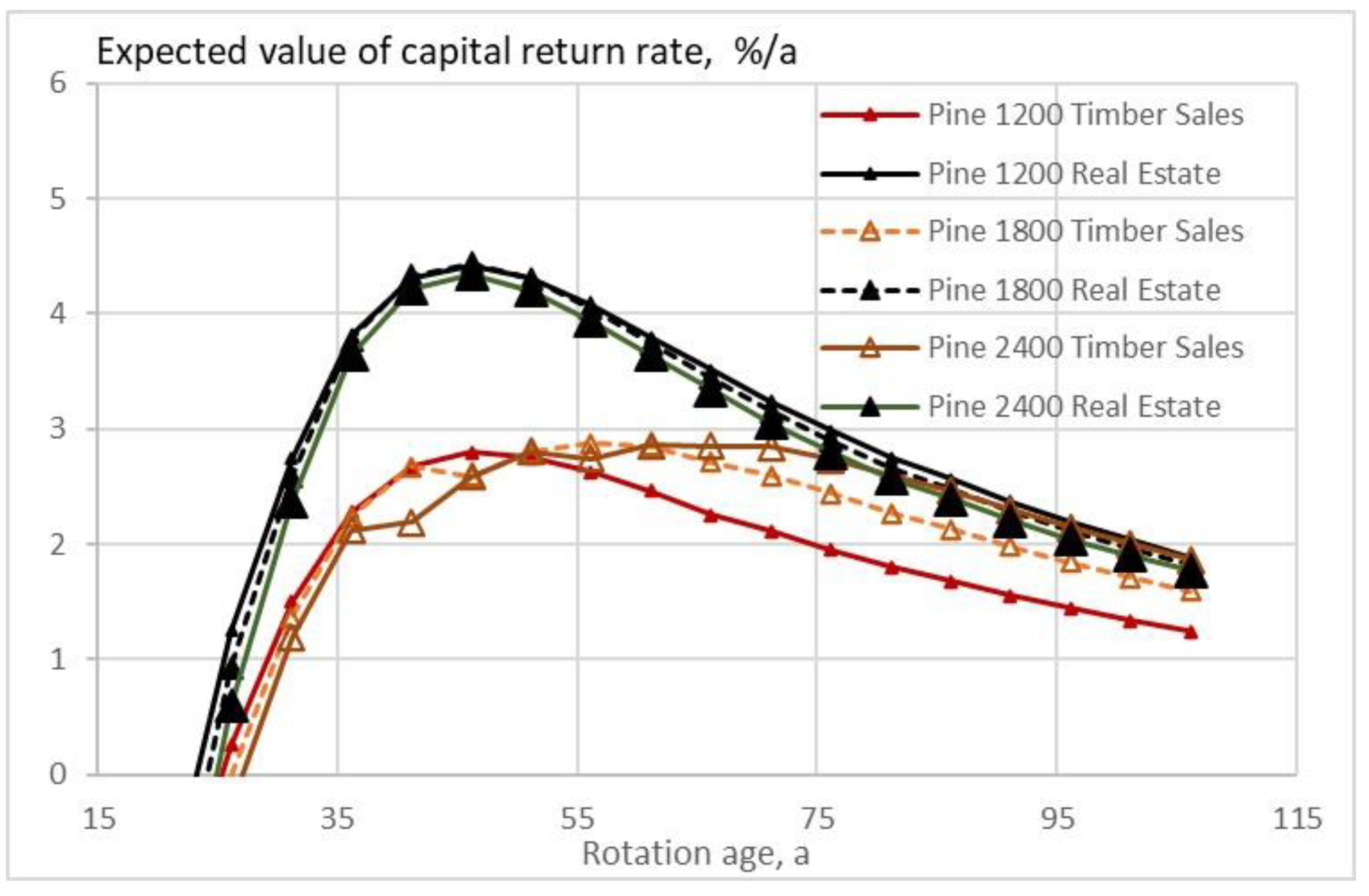
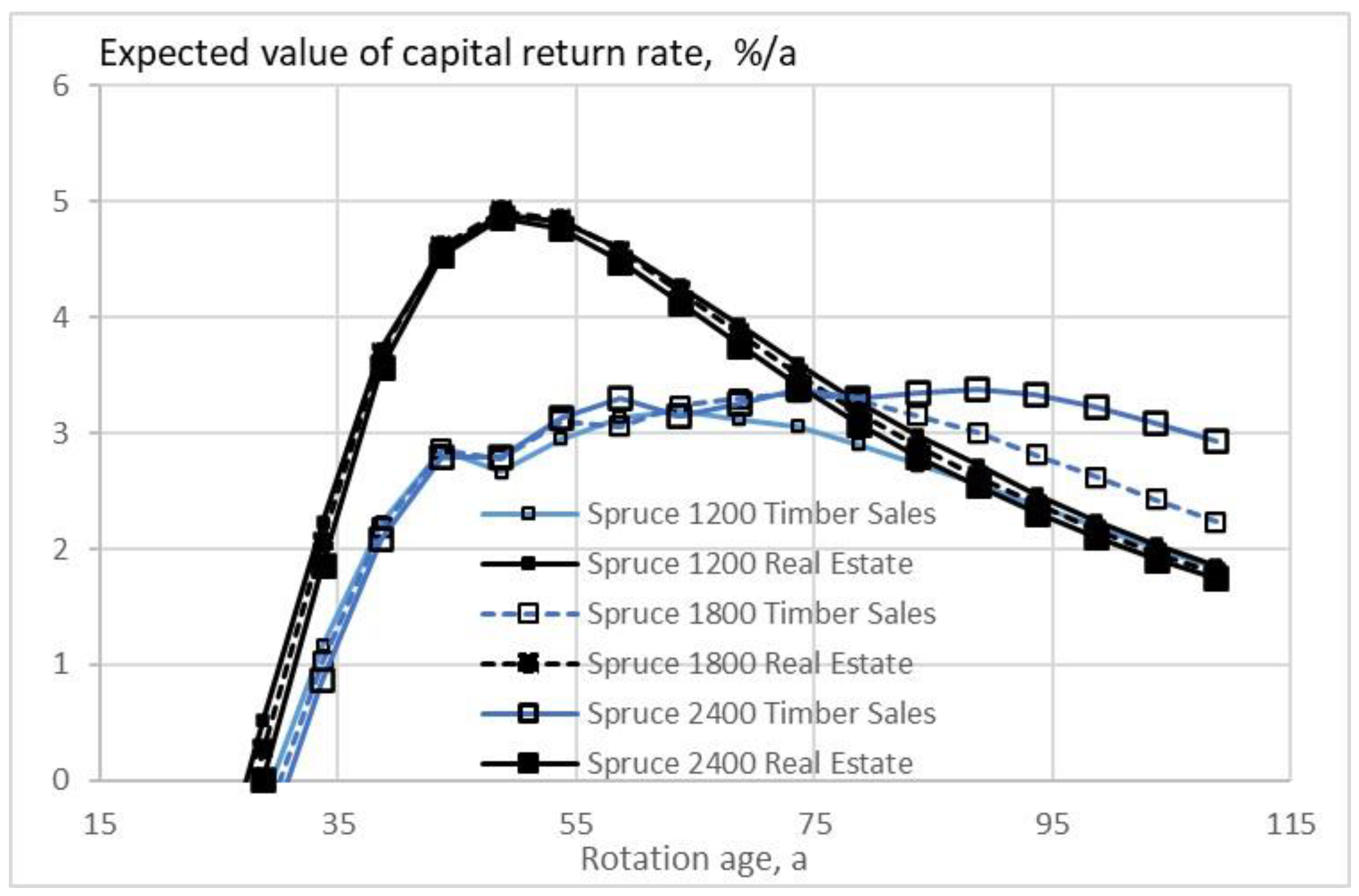
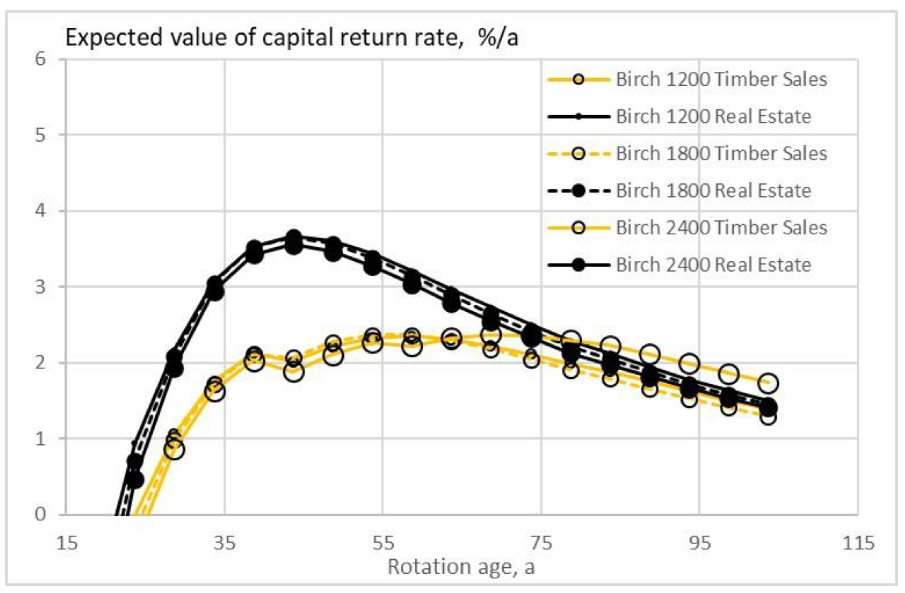
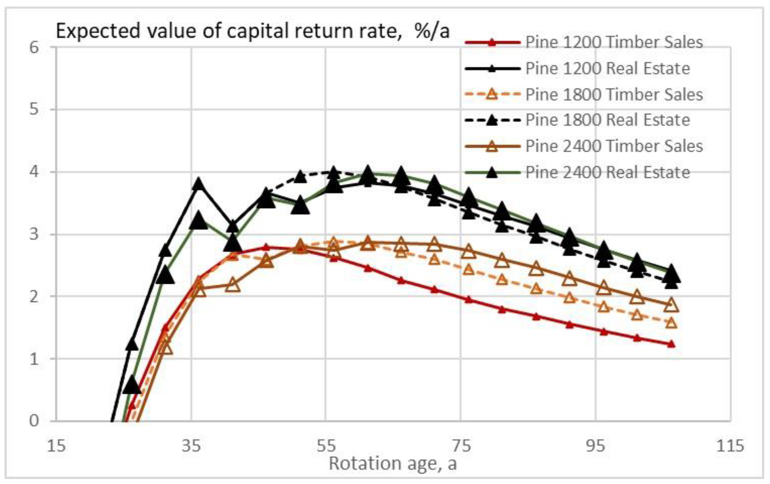
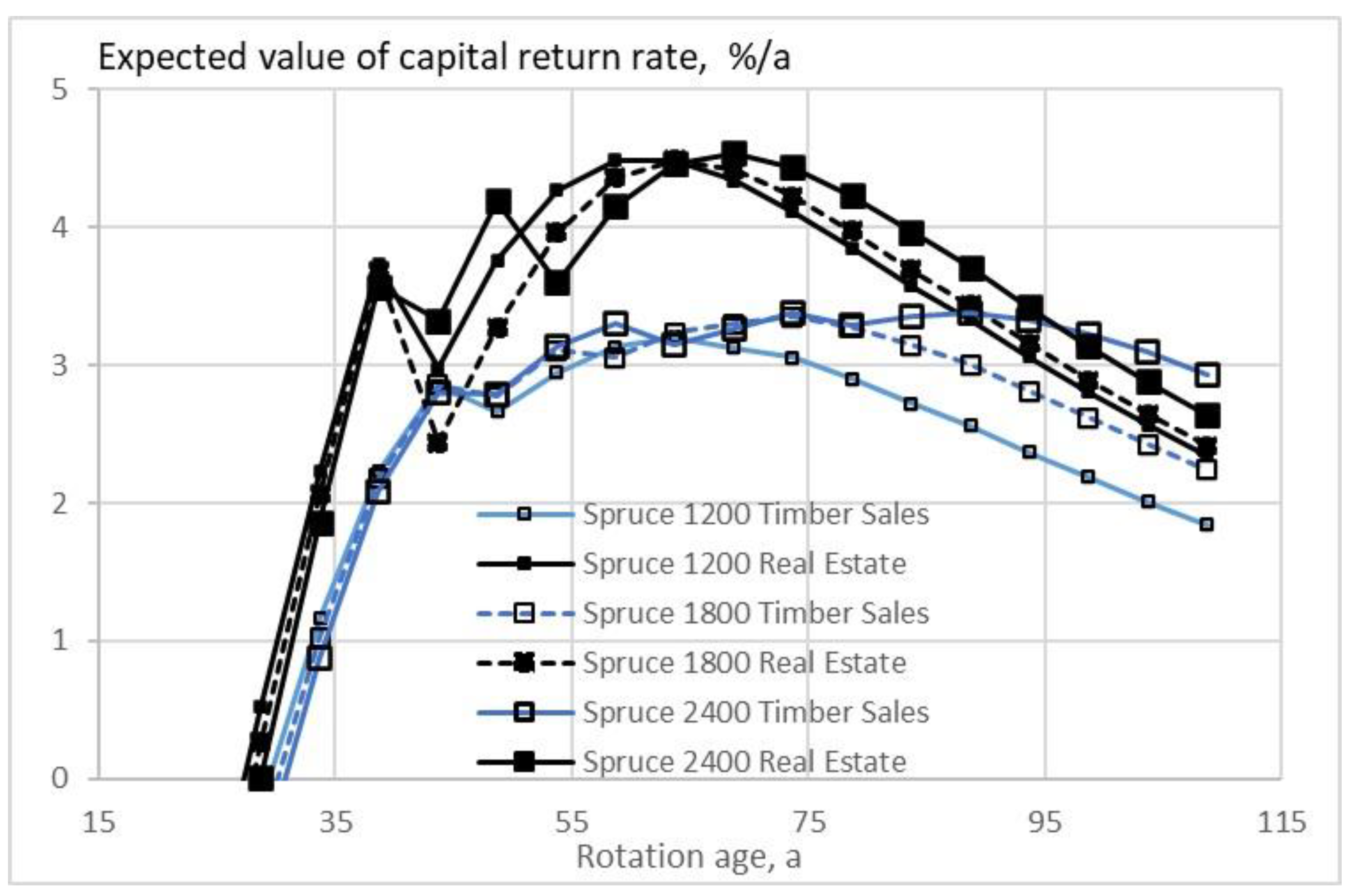
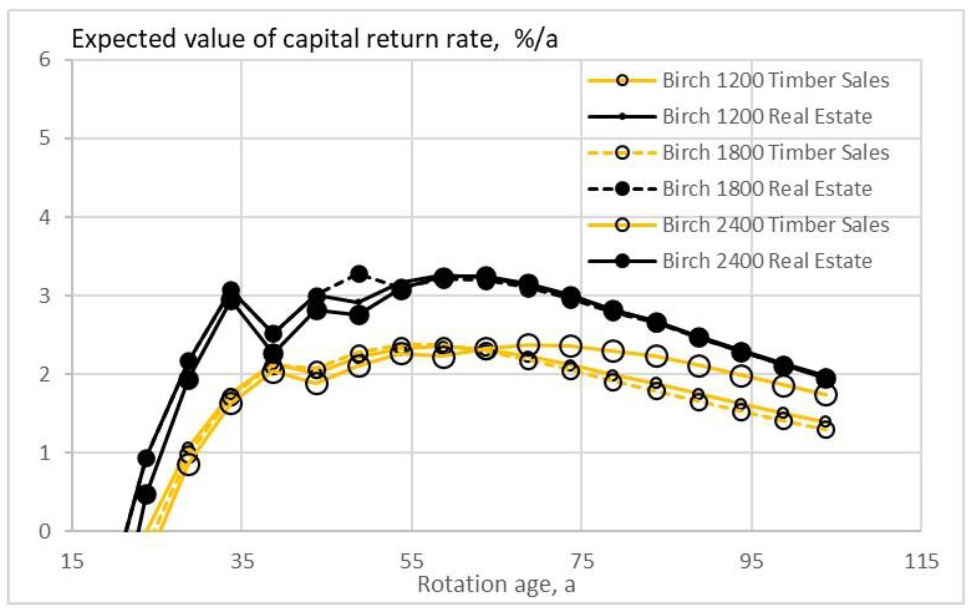
Figure 1, Figure 2 and Figure 3 show the expected value of the capital return rate within the stands of three tree species where the growth model is applied as early as applicable. In any of the three tree species, commercial thinnings do not enter the Real Estate strategy (Equation (8)). Stands to be harvested according to Timber Sales strategy (Equation (7)) do enter thinnings, with one exception. It is found that the achievable capital return rate is in the order of 50% greater in the Real Estate strategy, corresponding to shorter rotation ages.
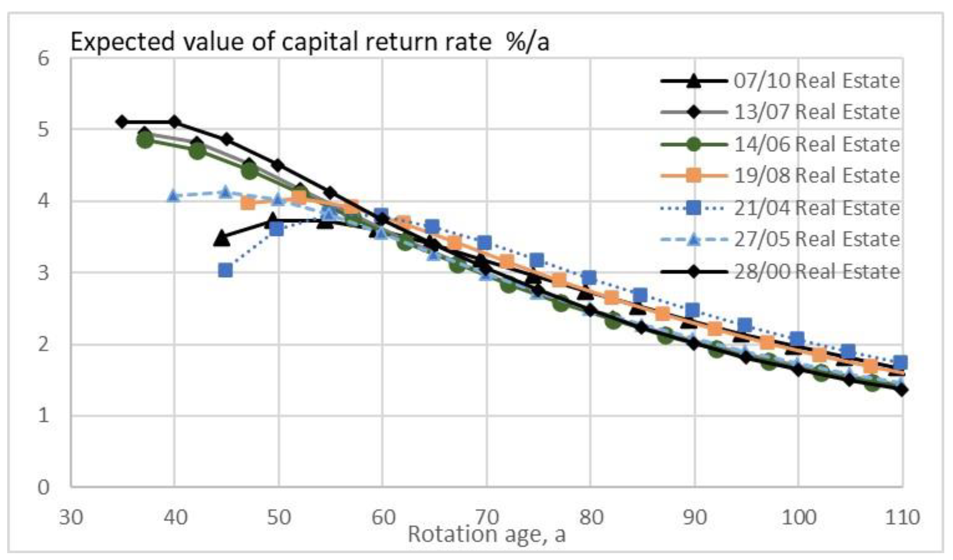
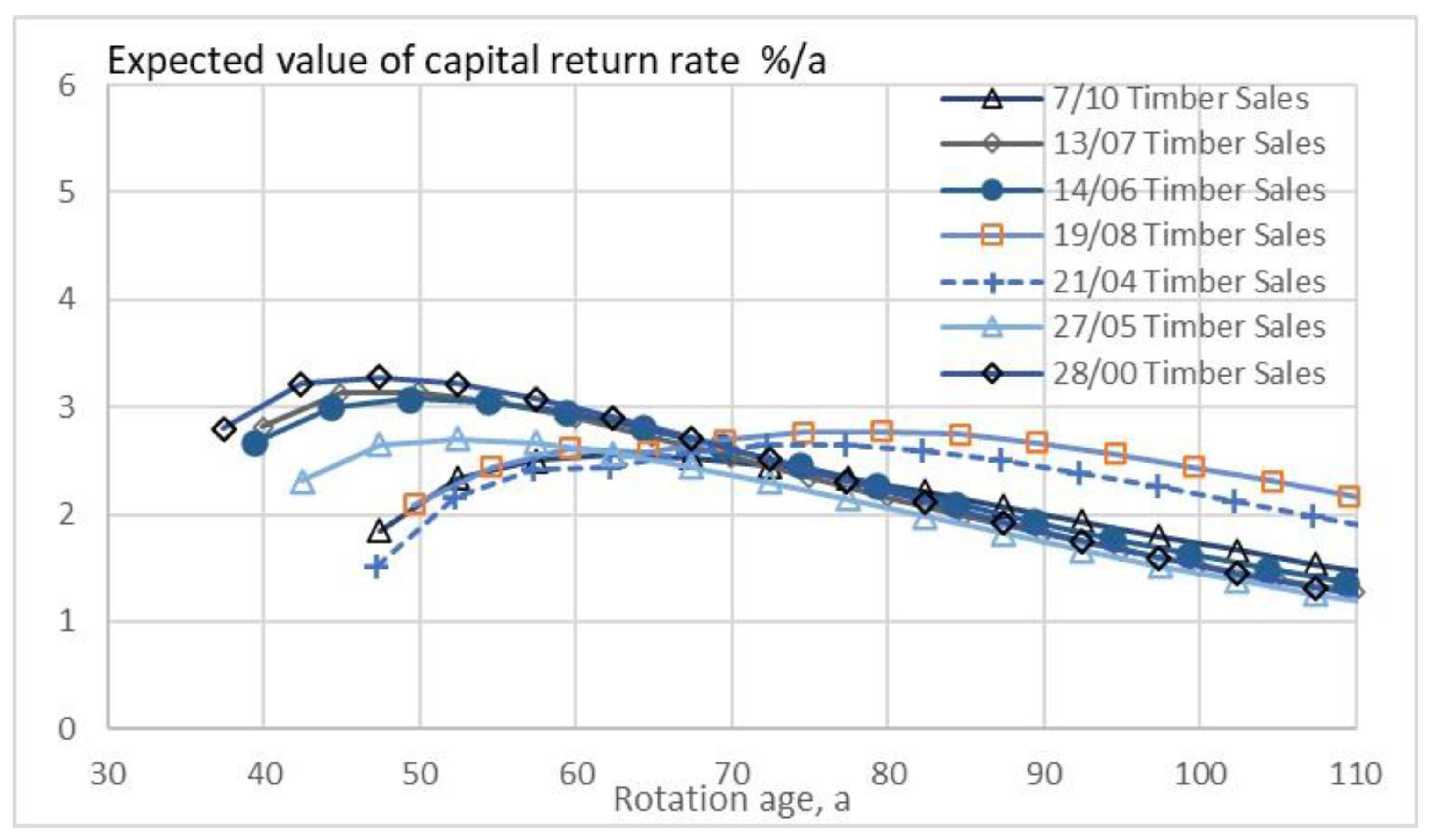
Figure 4 and Figure 5 show the expected value of the capital return rate within seven stands first observed at the age of 30 to 45 years, in the presence of inflated capitalization. The capital return rate according to Equation (8) within stands prepared for sale (Real Estate strategy, Figure 4) is consistently greater than that for stands to be harvested (Timber Sales strategy, Figure 5) according to Equation (7). No commercial thinnings are entered according to the RE strategy. Stands to be harvested according to the TS strategy (Equation (7)) always enter thinnings. The rotation times according to Equation (8) are consistently shorter, and capital return rates are in the order of 50% greater.
5. Discussion
It appears that either accepting or abandoning the periodic boundary condition of Equation (1) may result in dramatic consequences, as demonstrated above in Figure 1, Figure 2, Figure 3, Figure 4 and Figure 5. Such consequences depend upon the intangible market premium [8,9,10,11], applied as proportional to the tangible value [10,11,20]. The present author is not aware of earlier studies discussing the financial consequences of either accepting or abandoning a periodic boundary condition within a cyclical business.
According to the first-order approximation from Equation (8), the value extraction rate (or the rate of distributed dividends) differing from zero reduces the rate of return on capital. The computation of the example cases in Figure 1, Figure 2, Figure 3 and Figure 4 did not only contain the first-order approximation but the contribution to the capitalization appearing in the denominator of Equation (8) was also considered. Then, in Figure 1, Figure 2, Figure 3 and Figure 4, thinnings did not enter any of the solutions maximizing Equation (8). In other words, the extraction of capital value from the system within any rotation cycle was not recommended. The absence of thinnings corresponded to shorter rotation times in Figure 1, Figure 2, Figure 3 and Figure 4, in comparison to solutions based on Equation (7).
In terms of case studies, two strategies for boreal forestry have been discussed at stand level. The Timber Sales strategy can be naturally applied at stand level. The Real Estate strategy, however, possibly should be applied at the estate level. The stand-level treatment directly applies to even-aged estates. In the case of uneven-aged estates, robustness against varying rotation ages at the stand level would be beneficial.
Let us discuss the robustness of the Real estate strategy regarding rotation ages. It might be of interest to clarify the possibility of extending the rotation times within the RE strategy. It would allow older stands within an estate to hold while younger stands mature. On the other hand, such a possibility would create possibilities for selecting a suitable time for entering the real estate market, not necessarily directly due to the estate age structure.
A possibility for extending rotation ages within the RE strategy might be the application of commercial thinnings. Then, the cash flow (or the dividend rate) does not sum up to zero in Equation (8). In Figure 1, Figure 2, Figure 3 and Figure 4, the suitable rotation ages vary from 40 to 60 years, without thinnings. It is of interest how the rotation ages possibly could be extended by 20 years without any major loss of the expected value of capital return rate on the stand level.
It is found from Figure 6, Figure 7 and Figure 8 that in stands where the growth model is applied as early as applicable, thinnings from above can extend rotations with a minor loss in the financial return, and there is a significant difference between this modified RE strategy and the corresponding outcome of the TS strategy. The same partially applies to stands first observed at ages 30 to 45 years in Figure 9. However, in the case of fertile stands reaching the maximum financial return in Figure 4 soon after the time of stand observation, a greater loss results from the extension of the rotation time as is found in Figure 9. This possibly indicates that from the viewpoint of extending the rotation time, these stands are, at the time of observation, overdue for the best timing of thinning.
The example results of this paper are strictly applicable as long as the market premium in forest estates can be given in terms of proportional goodwill as introduced in Equations (7) and (8). In other words, the results are strictly valid as long as the intangible value premium can be given in terms of the scaling factor (1 + u). Such situations may vary with time, as well as between geographic areas. There are certainly occurrences where the goodwill values are temporarily disturbed on the market. However, observations indicate there is a long-term valuation trend in accordance with the proportional value premium [10,11,20].
Funding
This research was partially funded by Niemi Foundation.
Data Availability Statement
Conflicts of Interest
The author declares no conflict of interest.
References
- OECD. New sources of growth. In Measuring Innovation: A New Perspective; OECD Publishing: Paris, France, 2010. [Google Scholar] [CrossRef]
- Alsamawi, A.; Cadestin, C.; Jaax, A.; Guilhoto, J.; Miroudot, S.; Zürcher, C. Returns to Intangible Capital in Global Value Chains: New Evidence on Trends and Policy Determinants; OECD Trade Policy Papers, No. 240; OECD Publishing: Paris, France, 2020. [Google Scholar] [CrossRef]
- Kirca, A.H.; Hult, G.T.M.; Roth, K.; Cavusgil, S.T.; Perryy, M.Z.; Akdeniz, M.B.; Deligonul, S.Z.; Mena, J.A.; Pollitte, W.A.; Hoppner, J.J.; et al. Firm-specific assets, multinationality, and financial performance: A meta-analytic review and theoretical integration. Acad. Manag. J. 2011, 54, 47–72. [Google Scholar] [CrossRef]
- Bašić, M. Intangible assets and export growth of Croatian exporters: Evidence from panel VAR and VECM. Manag. J. Contemp. Manag. Issues 2023, 28, 201–210. [Google Scholar] [CrossRef]
- Hargrave, M. Goodwill (Accounting): What It Is, How It Works, How to Calculate. Available online: https://www.investopedia.com/terms/g/goodwill.asp (accessed on 11 December 2023).
- Miller, M.C. Goodwill-an aggregation issue. Account. Rev. 1973, 48, 280–291. [Google Scholar]
- Xu, L.; Guan, Y.; Fu, Z.; Xin, Y. Peer effect in the initial recognition of goodwill. China J. Account. Res. 2020, 13, 57–77. [Google Scholar] [CrossRef]
- Yao, W.; Mei, B.; Clutter, M.L. Pricing Timberland Assets in the United States by the Arbitrage Pricing Theory. For. Sci. 2014, 60, 943–952. [Google Scholar] [CrossRef]
- Korhonen, J.; Zhang, Y.; Toppinen, A. Examining timberland ownership and control strategies in the global forest sector. For. Policy Econ. 2016, 70, 39–46. [Google Scholar] [CrossRef]
- Viitala, E.-J. Stora Enson ja Metsäliitto-konsernin metsien omistusjärjestelyt vuosina 2001–2005. Metsätieteen Aikakauskirja 2010, 3, 239–260. [Google Scholar] [CrossRef]
- Mei, B. Timberland investments in the United States: A review and prospects. For. Policy Econ. 2019, 109, 101998. [Google Scholar] [CrossRef]
- Hu, X.; Jiang, C.; Wang, H.; Jiang, C.; Liu, J.; Zang, Y.; Li, S.; Wang, Y.; Bai, Y. A Comparison of Soil C, N, and P Stoichiometry Characteristics under Different Thinning Intensities in a Subtropical Moso bamboo (Phyllostachys edulis) Forest of China. Forests 2022, 13, 1770. [Google Scholar] [CrossRef]
- Seehuber, C.; Damerow, L.; Blanke, M.M. Concepts of selective mechanical thinning in fruit tree crops. Acta Hortic. 2013, 998, 77–83. [Google Scholar] [CrossRef]
- Rudnick, J.; Gaspari, G.; Privman, V. Effect of boundary conditions on the critical behavior of a finite high-dimensional Ising model. Phys. Rev. B 1985, 32, 7594(R). [Google Scholar] [CrossRef] [PubMed]
- Ryu, S.; Stroud, D. Magnetization Jump in a Model for Flux Lattice Melting at Low Magnetic Fields. Phys. Rev. Lett. 1997, 78, 4629. [Google Scholar] [CrossRef]
- Edwards, R.G.; Heller, U.M.; Klassen, T.R. Effectiveness of Nonperturbative O(a) Improvement in Lattice QCD. Phys. Rev. Lett. 1998, 80, 344. [Google Scholar] [CrossRef]
- Föllmer, H.; Schied, A. Probabilistic aspects of finance. Bernoulli 2013, 19, 1306–1326. [Google Scholar] [CrossRef]
- Busse, C.; Kach, A.; Wagner, S.M. Boundary Conditions: What They Are, How to Explore Them, Why We Need Them, and When to Consider Them. Organ. Res. Methods 2017, 20, 574–609. [Google Scholar] [CrossRef]
- Levendorskiĭ, S. Operators and Boundary Problems in Finance, Economics and Insurance: Peculiarities, Efficient Methods and Outstanding Problems. Mathematics 2022, 10, 1028. [Google Scholar] [CrossRef]
- Kärenlampi, P.P. Two Manifestations of Market Premium in the Capitalization of Carbon Forest Estates. Energies 2022, 15, 3212. [Google Scholar] [CrossRef]
- Kärenlampi, P.P. Harvesting Design by Capital Return. Forests 2019, 10, 283. [Google Scholar] [CrossRef]
- Kärenlampi, P.P. Diversity of Carbon Storage Economics in Fertile Boreal Spruce (Picea abies) Estates. Sustainability 2021, 13, 560. [Google Scholar] [CrossRef]
- Kärenlampi, P.P. Capital return rate and carbon storage on forest estates of three boreal tree species. Sustainability 2021, 13, 6675. [Google Scholar] [CrossRef]
- Kärenlampi, P.P. Two Sets of Initial Conditions on Boreal Forest Carbon Storage Economics. PLoS Clim. 2022, 1, e0000008. [Google Scholar] [CrossRef]
- Tilastotietoa Kiinteistökaupoista. Available online: https://khr.maanmittauslaitos.fi/tilastopalvelu/rest/API/kiinteistokauppojen-tilastopalvelu.html#t443g4_x_2020_x_Maakunta (accessed on 11 December 2023).
- Liljeroos, H. Hannun Hintaseuranta: Metsätilakaupan Sesonki Alkanut. Metsälehti 11.5.2021. Available online: https://www.metsalehti.fi/artikkelit/hannun-hintaseuranta-metsatilakaupan-sesonki-alkanut/#c8b05b17 (accessed on 11 December 2023).
- Kymmenen Prosentin Haamuraja Rikki—Metsäkiinteistöjen Hinnat Nousivat Ennätyksellisen Paljon Vuonna 2021. Suomen Sijoitusmetsät Oy, STT Info. Available online: https://www.sttinfo.fi/tiedote/kymmenen-prosentin-haamuraja-rikki-metsakiinteistojen-hinnat-nousivat-ennatyksellisen-paljon-vuonna-2021?publisherId=69818737&releaseId=69929002 (accessed on 11 December 2023).
- Bollandsås, O.M.; Buongiorno, J.; Gobakken, T. Predicting the growth of stands of trees of mixed species and size: A matrix model for Norway. Scand. J. For. Res. 2008, 23, 167–178. [Google Scholar] [CrossRef]
Figure 1.
The expected value of capital return rate on the pine (Pinus sylvestris) stands of different initial sapling densities, as a function of rotation age, when the growth model is applied as early as applicable, along with the Real Estate strategy (Equation (8)) and the Timber Sales strategy (Equation (7)).

Figure 2.
The expected value of capital return rate on spruce (Picea Abies) stands of different initial sapling densities, as a function of rotation age, when the growth model is applied as early as applicable, along with the Real Estate strategy (Equation (8)) and the Timber Sales strategy (Equation (7)).

Figure 3.
The expected value of capital return rate on birch (Betula pendula) stands of different initial sapling densities, as a function of rotation age, when the growth model is applied as early as applicable, along with the Real Estate strategy (Equation (8)) and the Timber Sales strategy (Equation (7)).

Figure 4.
The expected value of capital return rate, as a function of rotation age, when the growth model is applied to seven observed wooded stands, along with the Real estate strategy (Equation (8)). Thinnings do not enter. The numbers in legends identify stands and observation plots.
Figure 4.
The expected value of capital return rate, as a function of rotation age, when the growth model is applied to seven observed wooded stands, along with the Real estate strategy (Equation (8)). Thinnings do not enter. The numbers in legends identify stands and observation plots.

Figure 5.
The expected value of capital return rate, as a function of rotation age, when the growth model is applied to seven observed wooded stands, along with the Timber Strategy (Equation (7)). Thinnings do enter in all cases. The numbers in legends identify stands and observation plots.
Figure 5.
The expected value of capital return rate, as a function of rotation age, when the growth model is applied to seven observed wooded stands, along with the Timber Strategy (Equation (7)). Thinnings do enter in all cases. The numbers in legends identify stands and observation plots.

Figure 6.
The expected value of capital return rate on pine (Pinus sylvestris) stands of different initial sapling densities, as a function of rotation age, when the growth model is applied as early as applicable, along with the Real Estate strategy (Equation (8)) and the Timber Sales strategy (Equation (7)). Thinnings have been introduced into the RE strategy to extend the feasible rotations by 20 years.

Figure 7.
The expected value of capital return rate on spruce (Picea Abies) stands of different initial sapling densities, as a function of rotation age, when the growth model is applied as early as applicable, along with the Real Estate strategy (Equation (8)) and the Timber Sales strategy (Equation (7)). Thinnings have been introduced into the RE strategy to extend the feasible rotations by 20 years.

Figure 8.
The expected value of capital return rate on birch (Betula pendula) stands of different initial sapling densities, as a function of rotation age, when the growth model is applied as early as applicable, along with the Real Estate strategy (Equation (8)) and the Timber Sales strategy (Equation (7)). Thinnings have been introduced into the RE strategy to extend the feasible rotations by 20 years.

Figure 9.
The expected value of capital return rate, as a function of rotation age, when the growth model is applied to seven observed wooded stands, along with the Real Estate strategy (Equation (8)). The numbers in legends identify stands and observation plots. Thinnings have been introduced into the RE strategy to extend the feasible rotations by 20 years.

Disclaimer/Publisher’s Note: The statements, opinions and data contained in all publications are solely those of the individual author(s) and contributor(s) and not of MDPI and/or the editor(s). MDPI and/or the editor(s) disclaim responsibility for any injury to people or property resulting from any ideas, methods, instructions or products referred to in the content. |
© 2023 by the author. Licensee MDPI, Basel, Switzerland. This article is an open access article distributed under the terms and conditions of the Creative Commons Attribution (CC BY) license (https://creativecommons.org/licenses/by/4.0/).
Share and Cite
MDPI and ACS Style
Kärenlampi, P.P. Two Sets of Boundary Conditions in Cyclical Systems with Goodwill in Capitalization. Foundations 2024, 4, 3-13. https://doi.org/10.3390/foundations4010002
AMA Style
Kärenlampi PP. Two Sets of Boundary Conditions in Cyclical Systems with Goodwill in Capitalization. Foundations. 2024; 4(1):3-13. https://doi.org/10.3390/foundations4010002
Chicago/Turabian StyleKärenlampi, Petri P. 2024. "Two Sets of Boundary Conditions in Cyclical Systems with Goodwill in Capitalization" Foundations 4, no. 1: 3-13. https://doi.org/10.3390/foundations4010002