Lévy Walks as a Universal Mechanism of Turbulence Nonlocality

Abstract

The nonlocality (superdiffusion) of turbulence is expressed in the empiric Richardson t³ scaling law for the mean square of the mutual separation of a pair of particles in a fluid or gaseous medium. The development of the theory of nonlocality of various processes in physics and other sciences based on the concept of Lévy flights resulted in Shlesinger and colleagues’ about the possibility of describing the nonlocality of turbulence using a linear integro-differential equation with a slowly falling kernel. The approach developed by us made it possible to establish the closeness of the superdiffusion parameter of plasma density fluctuations moving across a strong magnetic field in a tokamak to the Richardson law. In this paper, we show the possibility of a universal description of the characteristics of nonlocality of transfer in a stochastic medium (including turbulence of gases and fluids) using the Biberman–Holstein approach to examine the transfer of excitation of a medium by photons, generalized in order to take into account the finiteness of the velocity of excitation carriers. This approach enables us to propose a scaling that generalizes Richardson’s t³ scaling law to the combined regime of Lévy flights and Lévy walks in fluids and gases.

1. Introduction: Superdiffusion in the Biberman–Holstein Model

The nonlocality (superdiffusion) of turbulence is expressed in the empirical Richardson t³ scaling law for turbulent relative dispersion, i.e., for the mean square of the mutual separation of a pair of particles, $r_{pair}\left(t\right)$, in a fluid or gaseous medium,

$$r_{pair}^2\left(t\right)\propto t^3.$$

(1)

This scaling was obtained within the framework of the diffusion model proposed by Richardson [1] (with the diffusion coefficient $K$ depending on distance r, $K\propto r^{4/3}$), suggested by the experimental data for atmospheric turbulence. Subsequently, the diffusion approach was developed in the direction of complicating the dependence of the diffusion coefficient. Along with this, the awareness of the phenomena of superdiffusion of turbulent dispersion came onto the scene, although Bachelor’s scaling [2], $r_{pair}^2\left(t\right)\propto t^2$, for ballistic motions is discussed only in connection with the initial stage of the separation of a pair of test particles. As a result, Richardson’s empirical scaling for pair correlations was derived in various models (see, for example, review [3]); however, at present, a nonlocal approach based on superdiffusion models is considered to be more adequate, in which, by the definition of superdiffusion, $r_{pair}^2\left(t\right)\propto t^{\beta }$, $\beta >1$. Within this framework, the concept of turbulence nonlocality is further developed, including attempts to reassess the Richardson scaling (1) itself (see [3]).

The key step in the development of the theory of nonlocality of various processes in physics and other sciences based on the concept of “Lévy flights”, introduced in [4] by Mandelbrot [5] (see [4,6,7,8]); moreover, “Levy walks” [9,10,11], which generalize Lévy flights to the case of taking into account the finite velocity of carriers, were the idea of Shlesinger and colleagues [10] for the possibility of describing the nonlocality of turbulence using a linear integro-differential equation with a kernel, slowly decreasing with distance. This approach suggests that the essentially non-linear dynamics of what we call turbulence can be reduced to the evolution of a statistical ensemble of carriers that have a large free path and, in fluid mechanics, can be associated with stable objects such as vortices/eddies. With this approach, the severity of complex nonlinear dynamics is transferred to the axiom of the existence of long-lived long-range motions in the medium, which are carriers of perturbations relative to some stable macroscopic state of the medium. The nonlocal transport of perturbations of the medium is assumed to be described by linear kinetic equations with the kernel of the integral operator, slowly decreasing with distance and belonging to the class of Lévy distributions.

In [12], an approach similar in spirit to [10] was proposed. The formalism of the type of the Biberman–Holstein equation [13,14] for the transfer of excitation by photons in gases and plasmas (for details, see, for example, [15,16]), generalized to consider the finiteness of the velocity of excitation carriers, was taken as a basis. Before formulating the model [12], it is appropriate to briefly describe the ideology of the Biberman–Holstein approach.

The basic equation for the excitation density of a medium in the problem of resonant radiation transfer is formulated for the density of excited atoms or ions $f\left(\mathbf{r},t\right)$. The Biberman–Holstein approach uses the approximation of complete redistribution (CRD) in a photon’s frequency in the elementary act of absorption of a photon by an atom or ion and re-emission of a photon in the same spectral line for the model of a two-level atom or ion, which is acceptable for the transfer of resonant radiation (generalization to the case of interdependent transfer of radiation in many spectral lines is easily feasible). The kinetic equation for the excitation density of the medium, in the case of stationary motionless unexcited medium, has the form:

$$\frac{\partial f\left(\mathbf{r},t\right)}{\partial t}=\frac{1}{\tau }{\int }_{V}W\left(\left|\mathbf{r}-{\mathbf{r}}_1\right|\right)f\left({\mathbf{r}}_1,t\right)d{V}_1-\left(\frac{1}{\tau }+\sigma \right)f\left(\mathbf{r},t\right)+q\left(\mathbf{r},t\right),$$

(2)

where τ is the lifetime of an excited atomic state with respect to spontaneous radiative decay; σ is the rate of collisional excitation quenching; q is the source of excitation of atoms, which is different from the excitation due to the absorption of a resonant photon (i.e., the source of collisional excitation). The kernel W is determined by the (normalized) spectral distribution of line emission source, ${\epsilon }_{\nu }$, and the absorption coefficient $k_{\nu }$, which is the inverse free path length (for the theory of spectral line shapes see [17,18,19,20,21,22,23]). Here, ${\epsilon }_{\nu }$ is specified as a function depending only on the parameters of the emitted photon (frequency and direction) and independent of the parameters of the absorbed photon, if the excited state was formed as a result of the absorption of the photon (i.e., there is the loss of memory by the excited atom about the prehistory of excitation). This feature of ${\epsilon }_{\nu }$ is a consequence of the CRD approximation mentioned above. In a homogeneous medium, W depends on the distance between the points of emission and absorption of a photon:

$$W\left(\rho \right)=-\frac{1}{4\pi {\rho }^2}\frac{dT\left(\rho \right)}{d\rho }\equiv \frac{1}{4\pi {\rho }^2}{W}_{step}\left(\rho \right), T\left(\rho \right)=\underset{0}{\overset{\infty }{\int }}{\epsilon }_{\nu }\exp \left(-k_{\nu }\rho \right)d\nu .$$

(3)

where the function $T\left(\rho \right)$, called the Holstein function (see [16] for an example), is the probability that a photon will freely travel a distance not less than $\rho$ without absorption. Thus, this function defines the distribution function for the carrier free path length, $W_{step}$ (step-length PDF). Accordingly, the kernel W, Equation (3), of the integral transport Equation (2) in three-dimensional coordinate space specifies the probability that the emitted photon will be absorbed at a distance $\rho$ from the point of photon’s birth. For practically interesting spectral-line-broadening mechanisms, including the Doppler effect and various mechanisms that give the Lorentzian form of the spectral line shape (spontaneous radiative decay, collisional perturbation of the excited state, including the dynamic Stark effect), the Holstein function at distances corresponding to large optical thicknesses, defined by the value of the absorption coefficient at the center of the spectral line ${\kappa }_0$, has a slow, power-law decay. For the Lorentzian (4) and Gaussian (i.e., Maxwellian Doppler) (5) shapes of the spectral line, one has [14]:

$$T\left(\rho \right)˜\frac{1}{\sqrt{\pi {\kappa }_0\rho }},$$

(4)

$$\begin{gathered} T\left(\rho \right)˜\frac{1}{{\kappa }_0\rho \sqrt{\pi \mathrm{l}\mathrm{n}\left({\kappa }_0\rho \right)}}, \\ {\kappa }_0\rho \gg 1. \end{gathered}$$

(5)

Nonlocality (superdiffusion) of radiation transfer, described by the Biberman–Holstein Equation (2), requires a special definition of the average time $\overline{t}(r)$, required for a photon to pass the distance r from an instantaneous point source q(r, t) = δ(r − r₀)δ(t − t₀). The commonly used concept of the average distance traveled by a photon in a given time turns out to be inapplicable in the case of superdiffusion, because the function f(r, t) falls too slowly with increasing distance from the primary source, and therefore the integral that determines the mean square of the displacement $\overline{r^2}$ diverges. The definition of $\overline{t}$(r) corresponding to the case of superdiffusion was given in [24] and takes the following form:

$$\overline{t}=\underset{0}{\overset{\infty }{\int }}dt\underset{0}{\overset{r}{\int }}d{r}_{1}4\pi r_1^{2}f\left(r_1,t\right).$$

(6)

In [24], analytical expressions for the asymptotic behavior of $\overline{t}$(r) (6) were obtained for two forms of the spectral line shape. For the dispersion (Lorentzian) form of the spectral line shape, we have the motion of the effective excitation front of the medium corresponding to the acceleration (r ∝ t²),

$$\overline{t}=3\tau \sqrt{{\kappa }_{0}r/\pi }=1.7\tau \sqrt{{\kappa }_{0}r}, t\gg \tau , {\kappa }_{0}r\gg 1,$$

(7)

And, for the Doppler form of the spectral line shape, the corresponding motion is almost free (r ∝ t ln(t/τ)):

$$\overline{t}=1.4\tau {\kappa }_{0}r\sqrt{\mathrm{l}\mathrm{n}\left({\kappa }_{0}r\right)}, t\gg \tau , {\kappa }_{0}r\gg 1.$$

(8)

Subsequently, in [25], it was indicated that both cases (7) and (8) are covered by a single formula,

$$\overline{t}\left(\rho \right)\approx \tau /T_{\mathrm{a}\mathrm{s}}\left(\rho \right),$$

(9)

where $T_{\mathrm{a}\mathrm{s}}\left(\rho \right)$ is given by (4) and (5).

When analyzing the transport for various mechanisms of spectral line broadening, it was shown [26] that the Biberman approximation [27], which makes it possible to reduce the equation integral with respect to coordinates to an algebraic one, is applicable the better, the slower the Holstein function decreases with increasing distance. The use of the approximation [27] in the theory of radiative transfer in one or many spectral lines is called the ${\tau }_{eff}$ method [28] or the escape probability method [29,30].

Equation (2) is integral over spatial coordinates and is not reducible to a differential equation: the term “diffusion” in the titles of some articles, including [24], is explained only as a tribute to the then existing terminology and does not correspond to the mathematical apparatus of diffusion. When the sought-for function $f\left({\mathbf{r}}_1,t\right)$ is expanded under the space integral in a Taylor series, in the case of an infinite volume of the medium, the diffusion coefficient turns out to be infinite, and in the case of a finite volume, it depends on the size of the medium (see, for example, [16]), which in principle contradicts the concept of diffusion. Despite the fact that the term Lévy flights had not yet penetrated into the theory of radiative transfer at the time of publications [15,16,29,30], the main transfer mechanism investigated in these theoretical approaches, in fact, refers specifically to Lévy flights.

An alternative to the Biberman–Holstein equation, which is widely used to describe laboratory plasma, is an approach often used in astrophysics, in which the pair of differential kinetic equations for photons and excited atoms/ions is reduced to an integral, in spatial variables, equation for the radiation intensity (see, e.g., [31,32,33,34,35]). Here, the dominant role of long free travels (i.e., Lévy flights) is also recognized, although usually without a proper name. The role of Lévy flights for light in the traditional radiative transfer in spectral lines was studied, for example, in [36]. Here, multiple scattering of near-resonant light in hot atomic vapors, characterized by Doppler broadening of the spectral line, experimentally confirmed theoretical studies [37], where it was shown that photon trajectories in the Biberman–Holstein model for the transfer of resonant radiation in spectral lines with Doppler, Lorentz, and Voigt broadening mechanisms contain Lévy flights.

The current state of the concept of Lévy flights and walks can be found in an extensive review [11], covering various fields of science. The latest results for Green’s function of the problem of nonstationary transfer of resonant radiation in the Biberman–Holstein model are presented in [38], including a generalization of the interpolated self-similarity method [39] to the case of a finite speed of light or other medium excitation carriers in [40,41,42]. Further progress in this direction led in [43] to the derivation of a unified approximate analytical description of the front of the nonstationary Green’s function for transfers in the Lévy flights and Lévy walks modes.

The results of these works served as an impetus to the application of the Biberman–Holstein model in two directions. In Section 2, we discuss the application to the interpretation of experiments on diagnosing plasma density fluctuations moving across a strong magnetic field in a tokamak [12] (as it turned out, tokamak plasma is a really turbulent medium in agreement with Richardson’s t³ law for hydrodynamic turbulence). In Section 3, a scaling is proposed, which generalizes Richardson’s law to the combined mode of Lévy flights and Lévy walks for hydrodynamic turbulence. One of the arguments in favor of the Biberman–Holstein approach is that it is another way to derive Richardson’s t³ law (1).

2. Superdiffusion in Plasma Turbulence

The study of superdiffusion processes in plasmas is of great practical interest. Thus, in studies of magnetically confined plasma for controlled thermonuclear fusion (primarily in the most successful direction, namely, in tokamaks), it has long been recognized that the process of heat transfer across a strong magnetic field is anomalous in the sense that the heat diffusion coefficients reconstructed from experimental data by solving inverse problems in the framework of diffusion models of transfer significantly (by one and a half to two orders of magnitude) exceed the predictions of theories from first principles. Therefore, in the interpretation of experiments and predictive modeling of plasma behavior, phenomenological models suggested by the results of experiments are used. These models are, as a rule, diffusion models, based on differential equations of the Fokker–Planck type in space variables. Attempts to construct models of nonlocal transfer from first principles have not yet given the desired agreement with the experiment. Let us point out, for example, the theory of non-stationary non-local heat transfer by longitudinal waves in plasma [44], brought to its final result for electron Bernstein waves (this method generalized the model of non-local transfer by electron and ion Bernstein waves [45] to the case of non-stationarity). Significantly greater success was achieved in the application of the above-mentioned escape probability method for the calculation of a separate component of the energy balance in tokamaks, namely, energy losses caused by the electron cyclotron radiation [46,47]. This approach extended and modified the approach [48,49,50] to heat transfer by electron cyclotron waves in thermonuclear plasmas (the current state of this issue can be found in [51]).

One way or another, the issue of diagnostics and predictive modeling of non-local transport remains essentially relevant. Therefore, of particular interest was an attempt [12] to prove the superdiffusion nature of the transfer of plasma density fluctuations across a strong magnetic field in tokamaks. Spectral and spatial characteristics of plasma density cross-correlations measured by probing the density fluctuations of a magnetized plasma with EM waves in the electron cyclotron frequency range were chosen as experimental data. The interest in the results of this diagnostics is due to the fact that in [52] (see also [53]) on the T-10 tokamak, almost symmetrical satellites of the main peak at the frequency of the probing radiation were discovered, which were called the quasi-coherent mode (QCM, see Figure 4a in [54]) and were then observed at other facilities, including tokamaks TEXTOR [55,56], Tore Supra [56], ASDEX Upgrade [57,58], KSTAR [59], HL-2A, and J-TEXT [60]. A feature of many experiments was that in order to measure the spectral and spatial characteristics of the cross-correlation (pair-correlation) function of the scattering of the probing EM wave, as was carried out in [52,53,54], the probing geometry (i.e., the direction of injection and of detection of the reflected EM wave) was such that the scattering vector (the difference between the wave vectors of the incident and reflected radiation) was directed across the strong magnetic field. This, as shown in [12], made it possible to diagnose the distribution function of fluctuations over the velocities of motion in this direction, obtaining a universal description of the relationship between the observed quasi-coherent mode in the spectrum of scattered EM waves and the process of the Mandelstam–Brillouin scattering type. It was also shown in [12] that the nonlocality of spatial correlations in a turbulent medium, which corresponds to the deviation of the pair correlation function of plasma density fluctuations from the Gaussian one, is due to long-range carriers of medium’s density fluctuations, for which the free path distribution function is described by the Lévy distribution. It was shown that the observed density fluctuations may be of turbulent origin, since the decay rate in the Levy distribution for the density fluctuation free path probability turned out to be close to its analogue, which gives Richardson’s empirical t³ law (1) for the hydrodynamic turbulence of fluids and gases. Below, we will dwell on the physical model [12] in more detail, since the success of its application to plasma turbulence will allow us to propose a generalization of Richardson’s law for fluids and gases in Section 3.

Let us consider a model of the microscopic dynamics of localized excitations of a medium (e.g., density perturbations) in a macroscopically quasi-homogeneous quasi-stationary medium. This model is an application of the Lévy walk concept to this class of problems. Similarly to the Biberman–Holstein model, we will consider two types of excitation of the medium, which can be transformed into each other. These two types can also be considered as different states (rest and motion) of the same object. This approach is applicable, for example, to biological migration, for which the applicability of the Lévy walk concept is well known (see, for example, review [11], section VI). In [61], a method was proposed and tested on synthetic experimental data for obtaining Green’s function of two-dimensional biological migration based on kinetic equations similar to those described below. The dominance of long-range movements (i.e., Lévy flights) corresponds to the fact that, for example, in search of food, animals try to escape from the place of the last stop as far as possible. Therefore, the trajectory of such motion topologically coincides with the trajectory of the excitation of the medium in the Biberman–Holstein model (compare, for example, Figure 1 in [43], Figure 1 in [61] and Figure 4 in [6]). This motion was called “Lévy walk with rests” (Figure 1 in [11]). In the model we are considering, it is precisely such motions that are meant; however, the common name is shortened to “Lévy walks”.

Let us consider a system of nonlocal transport equations for the intensity $I_{\tilde{\omega }}\left(\mathit{r},\mathit{n},t\right)$ (i.e., the energy flux density) of medium’s excitation carriers (e.g., running fluctuations of density) and standing excitations of the medium (e.g., standing fluctuations of density) $f(\mathit{r},t)$:

$$\frac{\partial f(\mathit{r},t)}{\partial t}=-\left(\frac{1}{\tau }+\sigma \right)f\left(\mathit{r},t\right)+\int d\tilde{\omega }\frac{{\kappa }_{\tilde{\omega }}\left(v\right)}{\hslash \tilde{\omega }}\int d\Omega \left(\mathit{n}\right)I_{\tilde{\omega }}\left(\mathit{r},\mathit{v},t\right)+q\left(\mathit{r},t\right),$$

(10)

$$\frac{\partial f(\mathit{r},t)}{\partial t}=-\left(\frac{1}{\tau }+\sigma \right)f\left(\mathit{r},t\right)+\int d\tilde{\omega }\frac{{\kappa }_{\tilde{\omega }}\left(v\right)}{\hslash \tilde{\omega }}\int d\Omega \left(\mathit{n}\right)I_{\tilde{\omega }}\left(\mathit{r},\mathit{v},t\right)+q\left(\mathit{r},t\right),$$

(11)

Let us describe the phenomenological functions and parameters included here, which should be restored by comparing the predictions of this model with experimental data.

Here, $\mathit{v}$ is the velocity of carriers of excitation, $\mathit{v}=\mathit{n}v$, which is assumed to be constant all the way between the point of birth and disappearance due to the transformation into a standing excitation of the medium. This means that we assume the existence of localized long-lived motions in a medium with a long free path, which are usually called solitons. An example of such motion in the two-dimensional case in plasmas and other media is the stable solutions of the nonlinear Kadomtsev–Petviashvili equation [62] (in the one-dimensional case, such an example is the Korteweg–de Vries equation). A discussion of general problems in the theory of solitons can be found, for example, in [63].

The source of standing excitations of the medium is given by the function $q\left(\mathit{r},t\right)$, which is the power density of the source of production of such excitation of the medium.

The spectral distribution of the probability of carrier’s emission with frequency $\tilde{\omega }$, normalized to the integral over frequency, is given by the function $P_{\tilde{\omega }}\left(v\right)$. The frequency (energy) and velocity of carriers are determined by the law of motion of the carrier (for linear waves in a homogeneous stationary medium, this relation is the law of wave dispersion).

The reciprocal length of the free path of the carrier from the point of birth to the stop in the medium and transformation into a standing excitation of the medium is given by the “absorption coefficient” of the carriers with the frequency $\tilde{\omega }$, ${\kappa }_{\tilde{\omega }}\left(v\right)$.

The average lifetime of standing excitation is given by the parameter τ, and the average reciprocal time of the disappearance of standing fluctuations without the creation of a carrier of excitation (the so-called “quenching” of the excitation of the medium) is given by the parameter σ.

The processes of generation of standing and running excitations of the medium are elementary mechanical processes in the sense that they exist as mutually inverse mechanical (i.e., reversible in time) processes. The proposed model assumes that standing excitation forgets the history of its occurrence. Equations (10) and (11) are written for carriers with a certain velocity, and it is assumed that there is some velocity distribution, which, like all other parameters and functions introduced above, can be restored by comparing the predictions of this model with experimental data.

Note that in the case of an infinite velocity of carriers (i.e., in the case of transfer in the Lévy flights mode), the system of Equations (10) and (11) reduces to the Biberman–Holstein Equation (2), and when this velocity is finite (i.e., in the case of transfer in the Lévy walk mode) instead of the function $f\left({\mathit{r}}_1,t\right)$ in (2) there is a function

$$\theta \left(t-\frac{\left|\mathit{r}-{\mathit{r}}_1\right|}{c}\right)f\left({\mathit{r}}_1,t-\frac{\left|\mathit{r}-{\mathit{r}}_1\right|}{c}\right)$$

(12)

(here, $\theta \left(x\right)$—the Heaviside step function), which takes into account the retardation. The derivation of such a generalization of the Biberman–Holstein equation from the system of Equations (10) and (11) can be found, for example, in Section 2 in [41].

An essential feature of the system of Equations (10) and (11) is that it is possible to reduce dependence of general solution, including practically interesting integral characteristics, only on the Holstein function. This means that such differential characteristics as the normalized spectrum of the source function, $P_{\tilde{\omega }}\left(v\right)$, and the reciprocal free path, ${\kappa }_{\tilde{\omega }}\left(v\right)$, enter the final result only as part of the Holstein function $T\left(x\right)$, defined in Equation (3). This feature of the system of Equations (10) and (11) is illustrated below by the following analytic results: general solution for Green’s function of excitation transfer in a three dimensional medium; effective front of Green’s function; pair correlation function (cross-correlation function) for the reflectometry of density fluctuations of the medium.

Firstly, in [42], the Fourier–Laplace transformation of (10) and (11) made it possible to obtain a solution for

$$q\propto \delta \left(\mathit{r}\right)\delta \left(t\right)$$

(13)

and a wide class of distribution functions over the free path of carriers (3) (step-length distribution function),

$$W_{step}\left(\rho \right)=\frac{\gamma {\kappa }_0}{{(1+{\kappa }_0\rho )}^{\gamma +1}}, 0<\gamma <2,$$

(14)

where ${\kappa }_0$ is a characteristic inverse length, which, in the case of excitation transfer by resonant photons, corresponds to the value of the absorption coefficient at the center of the spectral line. The choice of $W_{step}\left(\rho \right)$ in the form (14) makes it possible to cover a wide class of spectral line shapes including the Doppler and dispersion cases (see (7)–(9)). Indeed, the asymptotic behavior of (14) for ${\kappa }_0\rho \gg 1$ exactly coincides with that for the dispersion case and differs by a weak function $\sqrt{\mathrm{l}\mathrm{n}\left({\kappa }_{0}r\right)}$ for the Doppler case (cf. [24]). In the case of a variable velocity of carriers, the dependence ${\kappa }_0\left(v\right)$ makes $W_{step}\left(\rho ,v\right)$ (and $T\left(\rho ,v\right)$ according to (3)) a function of two arguments (see (23) in [12]). The obtained solution of Equations (10) and (11) as a function of dimensionless variables

$$r_d=r{\kappa }_0,\hspace{1em}\hspace{1em}{t}_d=t/\tau$$

(15)

explicitly depends only on the Holstein function (cf. Equation (2.20) in [42]):

$$f_{3D}\left(r,t,R_c\right)=\frac{1}{4{\pi }^3{r}_d i}\underset{0}{\overset{+\infty }{\int }}dp p \mathrm{s}\mathrm{i}\mathrm{n}\left(p{r}_d\right)\underset{+0-i\infty }{\overset{+0+i\infty }{\int }}\frac{e^{s{t}_d} ds}{s+1+\sigma \tau +\frac{1}{p}{\int }_0^{+\infty }\frac{dT\left(u\right)}{du}du e^{-su/R_c}\frac{\mathrm{s}\mathrm{i}\mathrm{n}\left(pu\right)}{u}},$$

(16)

where $R_c$ is the retardation parameter,

$$R_c=v\tau {\kappa }_0,$$

(17)

which is the ratio of the lifetime of the excitation of the medium at rest and in motion. Here, v is the fixed velocity of the carriers which in the case of radiative transfer equals to the speed of light.

Secondly, the dominant role of the Holstein function concerns the law of motion of the excitation front from a point instantaneous source, i.e., effective front of Green’s function. For Lévy flights the universal law was found in [25] (see (9)). For Lévy walks, i.e., in the case of a finite velocity of carriers, the respective results are presented in [43]. In contrast to the case of Lévy flights, where one has to work with the definition of the front in the form (6), for standing (and similarly for running) excitations of the medium, this front can be specified by a simple standard relation (cf. (3.1) in [43]):

$${\left(r_{rest}\left(t\right)\right)}^2=\left(\int r^2{f}_{rest}(\mathit{r},t)\mathit{d}\mathit{r}\right) / \left(\int f_{rest}(\mathit{r},t)\mathit{d}\mathit{r}\right),$$

(18)

since the numerator in (18) no longer diverges due to the limitation of distances by the ballistic motion front:

$$r_{ball}=vt.$$

(19)

For the front (18), as well as for the front of excitation carriers, in [43] for the distribution function over the free path of carriers (14) analytical expressions were obtained for practically interesting times and distances in transfer problems, namely for ${\kappa }_0\rho \gg 1$ and $t\gg \mathsf{\tau }$. The derivation of analytic results for Green’s function front for running excitation (i.e., excitation carriers) demanded derivation of a simple analytic description of the relationship between Green’s functions of the standing, $f_{rest}$, and running, $f_{mov}$, excitations of the medium. This possibility is suggested by the following general relation between these functions:

$$f_{mov}\left(\mathit{r},t,v\right)=\frac{1}{4\pi \tau v}\int \frac{d^3{r}_1}{{\left|\mathit{r}-{\mathit{r}}_1\right|}^2}T\left(\left|\mathit{r}-{\mathit{r}}_1\right|\right) \theta \left(t-\frac{\left|\mathit{r}-{\mathit{r}}_1\right|}{v}\right)f_{rest}\left({\mathit{r}}_1,t-\frac{\left|\mathit{r}-{\mathit{r}}_1\right|}{v}\right).$$

(20)

The possibility of simplifying this relation can be easily shown in the one-dimensional case, in which (20) takes the form

$$f_{mov}\left(x,t,v\right)=\frac{1}{2\tau v}\underset{-\infty }{\overset{+\infty }{\int }}d{x}_{1}T(\left|x_1\right|) \theta \left(t-\frac{\left|x_1\right|}{v}\right)f_{rest}\left(x_1+x,t-\frac{\left|x_1\right|}{v}\right).$$

(21)

If we assume that the function $f_{rest}$ changes slightly at distances that contribute to the integral over the coordinate, then we can neglect $x_1$ in the first argument. For the excitation density of the medium, it was shown in [43] that the propagation front defined as (18) does not depend on the spatial dimension of the problem. Therefore, to estimate such an integral characteristic as the propagation front of the medium’s excitation density, one can use the following approximate relation in the case of any space dimension:

$$f_{mov}(\mathit{r},t)=\frac{1}{\tau }\underset{0}{\overset{t}{\int }}d{t}^{\prime }{f}_{rest}\left(\mathit{r},t^{\prime }\right)T\left(v(t-t\prime )\right)$$

(22)

This approximation is close to the well-known Biberman approximation [27], in which a weak spatial dependence of the density of excited atoms on coordinates compared with the kernel of the integral operator in the Biberman–Holstein equation is assumed. This made it possible to remove the sought-for density from under the integral sign (recall that this approximation was later called the Escape Probability method [29,30]).

The validity of approximation (22) was proved in [43] by comparing the analytical formulas for the coordinate-integrated characteristics of Green’s function with the results of numerical calculations carried out in two different ways: (i) numerical integration of the general solutions for Green’s function and (ii) Monte Carlo numerical simulation of the solution of the same initial system of kinetic Equations (10) and (11). The results of such a comparison are shown in Figures 3–5 in [43].

Thirdly, in the problem of cross-correlation reflectometry of nonlocal characteristics of the transport of plasma density fluctuations in [12] a result was obtained, based on the system of Equations (10) and (11), for the spectrum of the cross-correlation function $\widehat{C}$, defined as a convolution (in fast time) of the electric fields $\mathit{E}$ scattered from two points ${\mathit{r}}_1$ and ${\mathit{r}}_2$ in the coordinate space:

$$C\left(\tilde{\tau },{\mathit{r}}_{\mathbf{1}},{\mathit{r}}_{\mathbf{2}}\right)=\frac{{\int }_{-\infty }^{+\infty }dt{\mathit{E}}^{*}\left({\mathit{r}}_{\mathbf{1}},t,{\mathit{K}}_{\mathbf{1}}\right)\mathit{E}\left({\mathit{r}}_{\mathbf{2}},t+\tilde{\tau },{\mathit{K}}_{\mathbf{2}}\right)}{{\left[{\int }_{-\infty }^{+\infty }dt{\left|\mathit{E}\left({\mathit{r}}_{\mathbf{1}},t,{\mathit{K}}_{\mathbf{1}}\right)\right|}^2{\int }_{-\infty }^{+\infty }dt{\left|\mathit{E}\left({\mathit{r}}_{\mathbf{2}},t,{\mathit{K}}_{\mathbf{2}}\right)\right|}^2\right]}^{1/2}}.$$

(23)

where $\mathit{K}={\mathit{k}}_{\mathit{s}}-{\mathit{k}}_{\mathit{i}}$ is the scattering wave vector, ${\mathit{k}}_{\mathit{i}}$ and ${\mathit{k}}_{\mathit{s}}$ are wave vectors of incident and scattered electromagnetic waves. Equation (23) is a standard definition of the cross-correlation function, which, for the problems of diagnosing a medium by probing with EM radiation, practically excludes the dependence of this function on the characteristics of the elementary act of interaction of probing radiation with those density fluctuations on which scattering occurs (for more details on the scattering of EM waves in plasma, see [64]).

The Fourier image of the function (23) is the outcome of the experimental data processing. In a more general form than in [12], it can be represented as follows (cf. (66), (67) in [12] for a homogeneous isotropic medium):

$$\widehat{C}\left(\omega ,{\mathit{r}}_2\to {\mathit{r}}_1\right)=e^{i\left(\mathit{K},\mathit{r}\right)}\frac{〈T\left(\left|{\mathit{v}}_{\mathbf{12}}\right|∆t_{12},{\mathit{v}}_{\mathbf{12}}\right)\mathit{exp}\left[i\left(\omega -\mathit{K}{\mathit{v}}_{\mathbf{12}}\right)∆t_{12}\right]\left|g\left({\mathit{r}}_2,\mathit{K},\omega ,{\mathit{v}}_{\mathbf{2}}\right)\right|〉}{{\left\{〈\left|g\left({\mathit{r}}_1,\mathit{K},\omega ,{\mathit{v}}_{\mathbf{1}}\right)\right|〉〈\left|g\left({\mathit{r}}_2,\mathit{K},\omega ,{\mathit{v}}_{\mathbf{2}}\right)\right|〉\right\}}^{1/2}}$$

(24)

where $\omega ={\omega }_s-{\omega }_i$, ${\omega }_i$ and ${\omega }_s$ are the frequencies of the of incident and scattered electromagnetic waves, $g\left({\mathit{r}}_1,\mathit{K},\omega ,{\mathit{v}}_{\mathbf{1}}\right)$ is the Fourier–Laplace image of the density of running fluctuation of the medium traveling with a velocity ${\mathit{v}}_{\mathbf{1}}$ at the point ${\mathit{r}}_{\mathbf{1}}$ (the Fourier transform with respect to the coordinate assumes the quasi-homogeneity of the medium at the point ${\mathit{r}}_{\mathbf{1}}$ on scales that allow an acceptable accuracy of calculating the Fourier transform so that a weak dependence on the spatial coordinate $\mathit{r}$ is present in all parameters in (10), (11), (14) such as $\sigma$, $\tau$, ${\kappa }_0$):

$$\check{g}\left(\mathit{K},\omega ,\mathit{v}\right)=\frac{Q\left(\mathit{K},i\omega ,v\right)}{4\pi \sigma \tau }\underset{0}{\overset{+\mathrm{\infty }}{\int }}dt e^{-i\left(\omega -\left(\mathit{v},\mathit{K}\right)\right)t}T\left(vt,\mathit{v}\right)$$

(25)

where $Q\left(\mathit{K},i\omega ,v\right)$ is the Fourier–Laplace image of the source function $q$ in (10), and we use an approximate expression for the effective source of standing excitations of the medium under the condition $\sigma \tau \gg \omega \tau \gg 1$ (cf. (40) and (41) in [12]).

The operator 〈…〉 in (24) means averaging over a given distribution in the velocities of running fluctuations. The delay time $∆t_{12}$ of the correlation between different points takes into account the finite velocity of the fluctuations, and in the case of a weak plasma inhomogeneity at a distance between the points under study, it is equal to

$$∆t_{12}=\left|{\mathit{r}}_1-{\mathit{r}}_2\right|/\left|{\mathit{v}}_{pl}+{\mathit{v}}_{\mathbf{12}}\right|,$$

(26)

where ${\mathit{v}}_{\mathbf{12}}$ is the velocity of density fluctuations between points 2 and 1 relative to the plasma (i.e., relative to the quasi-homogeneous hydrodynamic motion of the plasma in this region with the velocity ${\mathit{v}}_{pl}$).

This result (24) is also applicable to a homogeneous non-isotropic medium (such as, in particular, a homogeneous plasma in a uniform magnetic field).

The center of gravity of the cross-correlation function (24) is in the Holstein function (3), which determines the distribution function of running density fluctuations over their free path and depends—through the dependence ${\kappa }_0\left(v\right)$ in (14)—also on the fluctuation’s velocity. Function (24) is a spectrum of cross-correlations caused by the contribution of fluctuations that were ever at point ${\mathit{r}}_2$ to fluctuations of the same type found at point ${\mathit{r}}_1$ (the procedure for calculating the Fourier transform of the cross-correlation function is described in detail in [12]).

Formula (24), as shown in [65], retains its general structure for other types of cross-correlation diagnostics of plasmas, in which the measured medium characteristic (like the electric field of a scattered EM wave in reflectometry) is proportional to fluctuations of the plasma density. In this case, the frequency shift and the scattering wave vector in the problem of reflectometry are replaced by similar spectral-wave characteristics of signals measured by other diagnostics.

One of the main results of [12] is that for the first time the inverse problem of restoring the parameters of density fluctuations, on which probing radiation is scattered, was solved both for the spectral and radial dependence of the cross-correlation function $\widehat{C}\left(\omega ,∆r\right)$, where ∆r is the distance along the minor radius direction in the toroidal plasma column, i.e., across a strong toroidal magnetic field. The inverse problem was solved for the entire set of experimental data, including:

• The spectrum of scattered radiation (Figure 4a in [54]).
• The phase and the modulus of the complex function $\widehat{C}\left(\omega ,∆r\right)$ at fixed values of the distance between two points along the minor radius of the plasma column (Figure 4b,c in [54]).
• The coordinate dependence of $\widehat{C}\left(\omega ,∆r\right)$ at different frequencies.

An essential circumstance was that, for the first time, instead of the normal distribution usually used in the literature for the radial dependence of the cross-correlation function of reflectometry (see, for example, [54,66]), an analytical representation of the type (24) was used, which made it feasible to solve numerically the inverse problem of determining the parameters of plasma density fluctuations.

Finally, the most important consequence of the obtained solutions in [12] was that for the first time a characteristic was found for the degree of nonlocality of the motion of plasma density fluctuations across a strong magnetic field, which is described by the parameter γ in (14). It turned out that the value of the parameter γ ≈ 0.55 (see Figure 4 in [12]), found as a result of solving the inverse problem for the degree of nonlocality of the transfer of radially traveling plasma density fluctuations in the T-10 tokamak, is quite close to the value of the analogous parameter γ ≈ 2/3 in Richardson’s empirical law (1) for hydrodynamic turbulence. This was suggested by formulas (7.7) and (7.8) in [42] and is considered below in Section 3. The indicated closeness of the nonlocality parameter in plasma and fluid dynamics is an argument in favor of the fact that the observed dynamics of plasma density fluctuations can be of turbulent origin.

One might recall that it is much more difficult to measure Green’s function or the pair correlation function in plasma than in gases and fluids. Therefore, the results of plasma cross-correlation reflectometry are, apparently, the most powerful tool for analyzing the processes of transport of density fluctuations and, in particular, the extent to which these processes can be called turbulence.

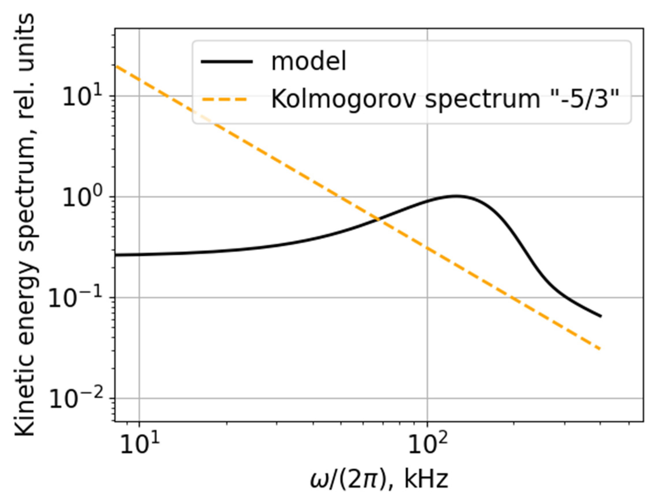
In addition to the results of [12], we present below the results of calculations of the fluctuation energy density spectrum and its comparison with the key result of Kolmogorov’s theory [67] for stationary homogeneous hydrodynamic turbulence.

The spectral distribution of the density of the kinetic energy of the fluctuating component of the velocity of the medium is defined as the Fourier transform of the square of the vector of this velocity (i.e., of the specific kinetic energy, defined as energy per unit mass). The calculation of this characteristic is one of the main results of the theory of hydrodynamic turbulence. Usually, this value is differential either in the modulus of the wave vector k (wavelength), or in the oscillation frequency ω. In fact, this means that we are talking about the Fourier–Laplace image of the specific kinetic energy of fluctuations, in which either the frequency ω or the modulus of the wave vector k is fixed and the differentiality in one of these parameters is somehow removed.

In the model referenced in [12], the analogue of this quantity is the product of the Fourier–Laplace image $\check{g}\left(\mathit{K},\omega ,\mathit{v}\right)$ (25) of the density of fluctuations and the square of their velocity. In the problem of reflectometry considered in [12], the wave vector is fixed by the experimental conditions, so it is appropriate for us to calculate the spectral distribution of the specific kinetic energy as a function of frequency at a given K. Since the results obtained in experiments with hydrodynamic turbulence do not depend on the primary source of disturbances in the medium, it is also appropriate for us to search for the spectrum regardless of the spectral characteristics of the primary source. Then, after averaging over the velocities, the final formula for the specific kinetic energy $\tilde{E}$ in the one-dimensional case of interest to us (the radial motion of fluctuations, distinguished by the measurement conditions in the experimental geometry in [54]) has the form:

$$\frac{d\tilde{E}}{d\omega }={\int }_{-\infty }^{+\infty }{v}_r^2 F\left(v_r\right)d{v}_r\left|\underset{0}{\overset{+\infty }{\int }}dt e^{-i\left(\omega -v_r{K}_r\right)t}T\left(\left|v_r\right|t,\left|v_r\right|\right)\right|,$$

(27)

where $T\left(r,v\right)$ is the Holstein function that specifies the distribution function over the free path (3) of plasma density fluctuations moving with velocity $v_r$ along the direction under study, $K_r=\left|\mathit{K}\right|$ is the radial component of the scattering vector, $F\left(v_r\right)$ is the distribution function of velocity fluctuations along the minor radius of the toroidal plasma column, specified by (51) in [12] and corresponding to the motion of density fluctuations with velocities near a characteristic velocity along and against the direction of observation in experiments [54]. It is this distribution over the radial velocity that can give the spectrum of the scattered EM field in these experiments (see Figures 1 and 5 in [12]).

In the case of weak broadening of the spectrum due to the finiteness of the mean free path of running fluctuations, the time integral in (17) is close to the Dirac delta-function (compare Figures 1 and 2 in [12]). Therefore, frequency distribution (17) of the specific kinetic energy—similar to the spectrum of scattered radiation during reflectometric probing of plasma—approximately coincides with the velocity distribution of fluctuating motions of the medium in the regime of hydrodynamic turbulence. In hydrodynamics, this spectrum has a wide range of power-law decay in the so-called inertial interval, Kolmogorov’s 5/3 law, confirmed by experimental data for the spectral distribution (see, for example, Figure 3 in [68]). In the inertial interval, the influence of the turbulence source (pumping) and sink on the spectrum can be neglected. The upper limit of this interval corresponds to the minimum distances at which viscous losses can still be neglected. The role of viscosity, as suggested in [67], is reduced to maintaining a stationary flow in the space of wave numbers due to the transformation of hydrodynamic vortices into smaller ones (a unidirectional, “direct” cascade of vortices).

Based on the solution [12] of the inverse problem of reconstructing the turbulence nonlocality parameters, using (24), from the experimental data for the cross-correlation reflectometry of the tokamak T-10 plasma, it is possible to calculate the spectral distribution of the specific kinetic energy for the set of parameters listed in [12], Section 6.1, before Figure 1 (see also Figures 1–4 in [12]). Note that the optimal value of the nonlocality parameter is $\gamma =0.55$, and the dependence on this parameter is shown in Figure 4 in [12]. Figure 1 shows a comparison of the spectrum (27) with Kolmogorov’s 5/3 scaling law in logarithmic coordinates. We note that the high-frequency asymptotic behavior of the spectrum coincides with Kolmogorov’s law, and the general form of the spectrum is close, for example, to the results in Figure 18 in [69].

Thus, not only the proximity of the nonlocality parameter γ, obtained in [12], to the corresponding parameter for the Richardson t³ law (1), but also the similarity of the spectrum of the specific kinetic energy of density fluctuations in the tokamak plasma to the spectrum of the fluctuation velocity component in hydrodynamic turbulence make it possible to qualify the transport of density fluctuations in a tokamak plasma across a strong magnetic field as turbulence. Note that studies of the nonlocal properties of turbulence, including the deviation of statistics from the Gaussian one in various plasma turbulence phenomena, are reflected in the collective monograph [70].

The phenomenological model [12] of turbulence nonlocality, based on the system of kinetic Equations (10) and (11) and going beyond the diffusion Fokker–Planck models, can be considered, when applied to plasma, as a phenomenological generalization of the quasilinear theory of weak plasma turbulence, which goes back to [71], in the wave part of this kinetics (a review of the status of the quasilinear approach to plasma turbulence is presented in [72]). Going beyond the diffusion Fokker–Planck models has already been made, and for specific physical models in the case of a stationary flow in the space of wave numbers (not the thermodynamic limit), examples of the Kolmogorov spectrum in various problems of physics have been found [73]. In the problem considered in [12] and here, it is important that it was possible to establish the closeness of the kinetics of plasma density fluctuations to what we call turbulence within the general framework of interpreting the results of experiments, without specifying the physical model of elementary excitations of the medium.

A successful attempt to numerically simulate from first principles (within the framework of the gyrokinetic approach) the dynamics of fluctuations of plasma parameters and the corresponding spectrum of scattered radiation during reflectometry in the Tore Supra tokamak was undertaken in [74]: the coincidence of the results of numerical simulation of the spectrum with the measured strongly pronounced structure of the quasi-coherent mode made it possible to assume the origin of turbulence due to the dominance of certain plasma wave modes. However, we do not yet know examples of measurements and corresponding numerical simulations of the cross-correlation function $\widehat{C}\left(\omega ,∆r\right)$ in full, similar to the full set of the results in Figures 4, 5 and 13 in [54] or Figures 1–4 in [12].

3. Extension of Richardson’s t³ Law to the Combined Lévy Flight and Lévy Walk Regime for Turbulence in Fluids and Gases

The hypothesis of the locality of elementary processes in the existing quasi-linear theory of weak plasma turbulence seems to be quite justified, since for elementary processes it is possible to propose mechanical (i.e., reversible in time) models from first principles. For hydrodynamic turbulence, this aspect inevitably requires additional axiomatics, which obviously are the well-known hypotheses of Kolmogorov and Obukhov for homogeneous stationary turbulence. Lack of rigorous justification, i.e., the lack of a derivation from the Navier–Stokes equations sometimes allows researchers to qualify this approach as dimensional reasoning. Therefore, in the existing rather free field in the theory of hydrodynamic turbulence, it is quite legitimate to propose other models with their own axiomatics. Such an attempt is the generalization of Richardson’s t³ law (1) given below to the combined regime of Lévy flights and Lévy walks. Such a generalization is suggested, as noted above, by the idea of Schlesinger and colleagues [10] and the success of the model [12] in interpreting experiments on cross-correlation reflectometry of tokamak plasma.

Let us turn to the model (10), (11) with the intention of establishing a connection between the phenomenological parameters introduced in it and the key parameters of the existing theory of hydrodynamic turbulence. It is important to note that although model (10), (11) did not discuss the possible physical mechanisms of elementary acts in the kinetic model, such possibilities in the theory of linear waves are well known and form the basis of the already mentioned quasilinear theory of weak plasma turbulence. The problem, however, lies in the fact that models of superdiffusion transfer of energy by linear plasma waves have not yet been created, which would provide explanations for the observed nonlocality phenomena, for example, in thermonuclear plasma (for example, we repeat the reference to [44,45], but this list can be continued up to the present moment). Therefore, the problem of identifying adequate elementary acts responsible for the observed phenomena of superdiffusion transfer is to a comparable extent faced by both the theory of turbulent plasma and the theory of non-plasma hydrodynamic turbulence.

In this section, we will not solve the latter problem, but will only draw a bridge between the phenomenology of plasma and non-plasma hydrodynamic turbulence.

For hydrodynamic turbulence of fluids and gases, the key parameters are the Kolmogorov length $\mathsf{\eta }$ and velocity $v_{\mathsf{\eta }}$, as well as the corresponding time $t_{\mathsf{\eta }}$:

$$\eta ={\left({\nu }^3/{\epsilon }_0\right)}^{1/4},\hspace{1em}{v}_{\eta }={\left(\nu {\epsilon }_0\right)}^{1/4},\hspace{1em}{t}_{\eta }={\left(\nu /{\epsilon }_0\right)}^{1/2},$$

(28)

where $\nu$ is the kinematic viscosity in units of m²/s, ${\epsilon }_0$ characterizes the specific energy dissipation rate in units of m²/s³.

Let us propose analogs of the Kolmogorov parameters in a kinetic transport model of the Biberman–Holstein type with allowance for retardation. An analogue of the Kolmogorov length is the path length at the center of the spectral line, ${\kappa }_0$, since, as in the Kolmogorov model, is the minimum characteristic length:

$$\frac{1}{{{(\kappa }_0)}_{turb}} ˜ \eta .$$

(29)

Of course, relations (29)–(31) have the meaning of equality in order of magnitude.

An analogue of the Kolmogorov velocity is the characteristic velocity of running excitations of the medium (carriers). Batchelor’s scaling for the initial stage of mutual separation of closely spaced test particles works in favor of the analogy for velocities:

$${\left(r_{pair}\left(t\right)\right)}^2 ˜ {\left(v_{\mathsf{\eta }}t\right)}^2˜ {\left(vt\right)}^2.$$

(30)

In the plasma turbulent motions along the minor radius of a toroidal plasma in a tokamak, this corresponds to a characteristic velocity restored [12] from the observed peaks in the spectrum of the quasi-coherent mode. Since $t_{\mathsf{\eta }}$ has a simple relationship with $\eta$ and $v_{\eta }$, we can put

$${\tau ˜t}_{\eta }.$$

(31)

To estimate the pair correlation function (turbulent relative dispersion) in order of magnitude, which is acceptable considering the status of such an integral estimate of the distribution function in kinetic problems, we will use the analytical approximation results for Green’s function of the nonlocal transfer in the combined mode of Lévy flights and Lévy walks, according to (7.10) in [43], for step-length PDF in the form (14):

$${\left(\frac{r_{pair}\left(t,R_c,\gamma \right)}{\eta }\right)}^2˜\frac{1}{{\left(\frac{t_{\eta }}{t}\right)}^{2/\gamma }+{\left(\frac{t_{\eta }}{t}\right)}^2 \frac{1}{{R_c}^2}\left(\frac{1+\gamma }{1-\gamma }\right)},$$

(32)

where $R_c$ is the retardation parameter,

$$R_c=c\tau {\kappa }_0,$$

(33)

which is the ratio of the lifetime of the excitation of the medium at rest and in motion (here c is the characteristic velocity of the carriers). With the specified correspondence to the Kolmogorov turbulence parameters (28), $R_c$ can be determined to be a certain number in the range determined by the accuracy of estimates (29)–(31), i.e., some free parameter. Preservation of the last factor in the second term in the denominator in (32) ensures that the front velocity (turbulent pair dispersion) is less than the ballistic limit (19).

Note that the proposed scaling (32) covers only the transition between transfers in the Lévy flight and Lévy walk modes. To construct a more general scaling, it is necessary to take into account the Batchelor ballistic regime at the initial stage and the diffusion regime at the final stage; see Figures 5–7 in [75].

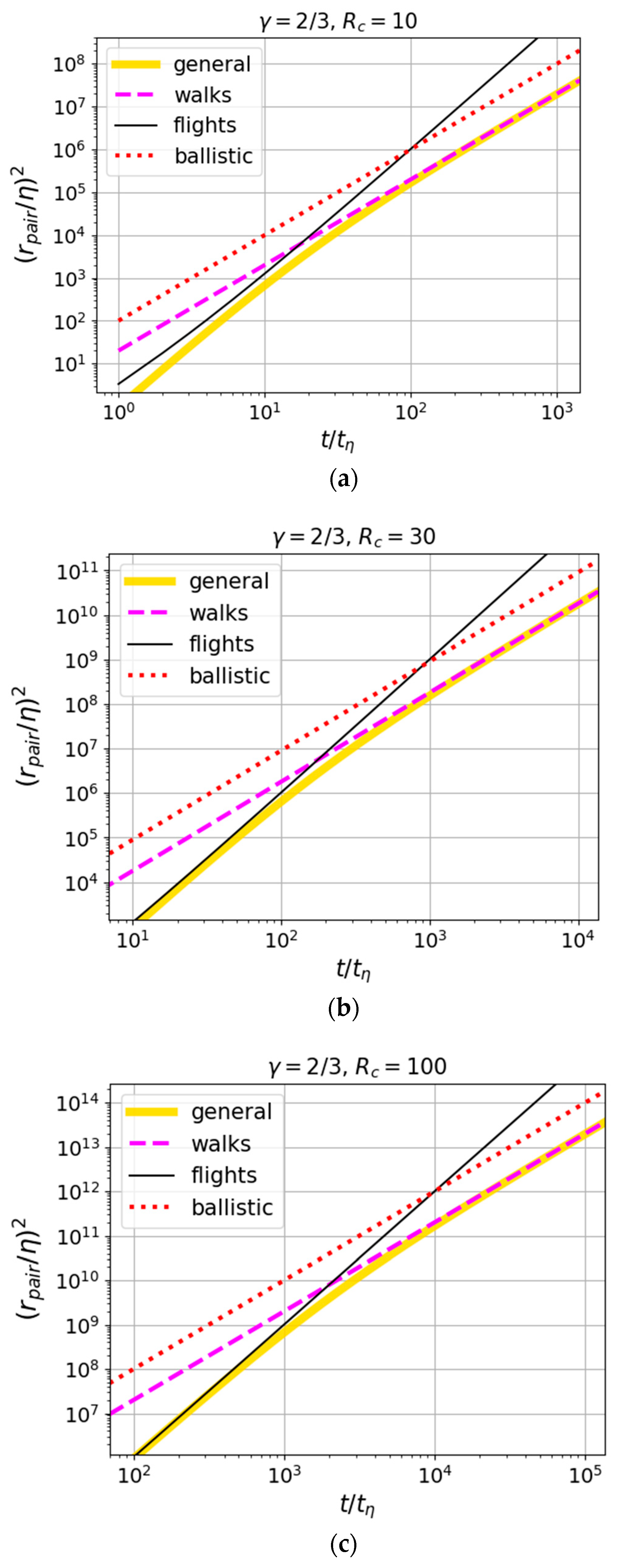
For γ = 2/3, we obtain from (32):

$${\left(\frac{r_{pair}\left(t,R_c,\gamma \right)}{\eta }\right)}^2˜\frac{{\left(\frac{t}{ t_{\eta }}\right)}^3}{1+5\left(\frac{t}{ t_{\eta }}\right) \frac{1}{{R_c}^2}},$$

(34)

If the retardation effect is neglected (i.e., $R_c\to \infty$), Richardson’s law (1) is obtained from (34). Calculations of (34) are shown in Figure 2 for various values of the retardation parameter. Comparison with the results of numerical simulations in [75], where Richardson scaling (1) works up to time $t˜{{10}^{2}t}_{\mathsf{\eta }}$, shows that a possible niche exists for taking into account the retardation and the respective appearance of ballistic scaling of Lévy walks with a value of the retardation parameter $R_c$ equal to few–several tens. This niche is in the intermediate region between Richardson scaling (1) and diffusion scaling ${\left(r_{pair}\right)}^2\propto t$ at very large values of $t/t_{\mathsf{\eta }}$.

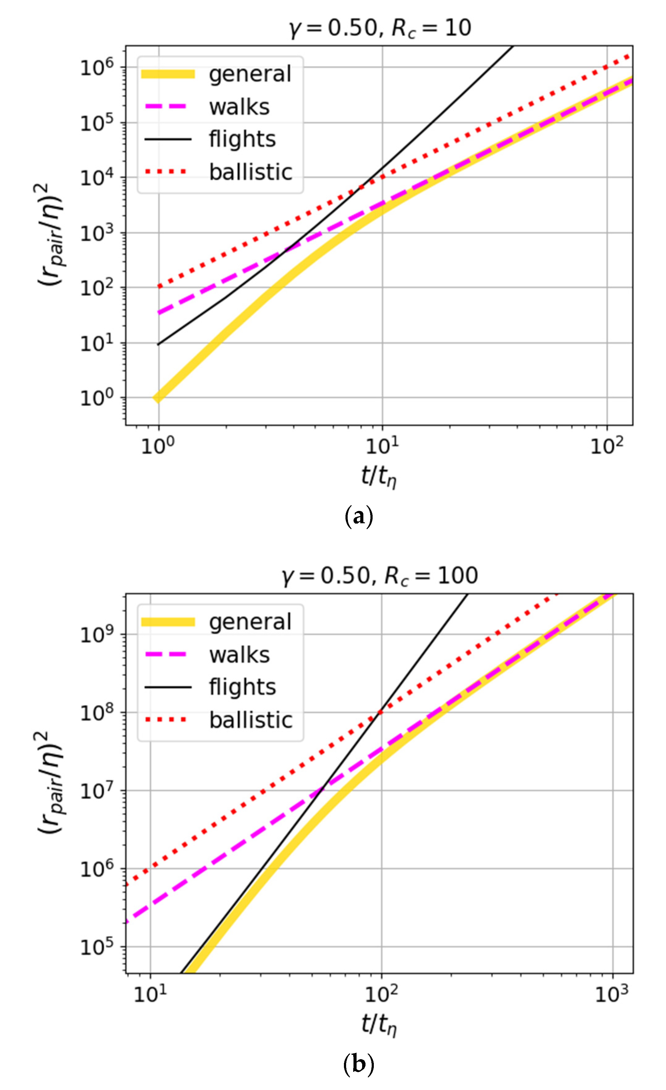
The faster growth of the pair correlation with time, obtained in simulations [75] in the regions where the Richardson law (1) was expected (i.e., between the Batchelor ballistic regime and the diffusion regime, see Figure 7 in [75]), suggests that the case of smaller values of the nonlocality parameter $\gamma$ may also be considered, for example, $\gamma =1/2$. This choice is also interesting in that the spectral probability density shape $P_{\tilde{\omega }}$ corresponding to this case in model (10), (11) has a Lorentzian form, which often occurs in various physical models, where the broadening of the spectral distribution compared with the monochromatic one is due to the finiteness of the lifetime of the excited state, the relaxation of which leads to the birth of a carrier (running excitation of the medium). In the case of $\gamma =1/2$, from (32), we obtain:

$${\left(\frac{r_{pair}\left(t,R_c,\gamma \right)}{\eta }\right)}^2˜\frac{{\left(\frac{t}{ t_{\eta }}\right)}^4}{1+3{\left(\frac{t}{ t_{\eta }}\right)}^2 \frac{1}{{R_c}^2}}.$$

(35)

Calculations by Formula (35) for various values of the retardation parameter are shown in Figure 3. Comparison with the results of numerical simulations in [75], where Richardson scaling (1) works up to time $t˜{{10}^{2}t}_{\mathsf{\eta }}$, shows that a possible niche for taking into account the retardation and the respective appearance of the ballistic scaling of Lévy walks exists for the retardation parameter $R_c$ of the order of ${10}^2$. In this case, the scaling ${\left(r_{pair}\right)}^2\propto t^4$ works up to $t/t_{\mathsf{\eta }}˜{10}^2$ where the transition to ${\left(r_{pair}\right)}^2\propto t^2$ occurs with a possible transition to diffusion scaling at larger values of $t/t_{\mathsf{\eta }}$ (cf. Figure 7 in [75]).

Thus, the kinetic model (10), (11) allows us to qualitatively consider the problem of expanding the range of applicability of the Richardson law (1) and the problem of its possible generalization and reassessment, which, in particular, was actively discussed in [3]. Although Richardson’s t³ law (1) is supported by an extensive database, including, for example, recent experimental and theoretical studies in [76], the behavior of turbulent pair correlation (turbulent pair dispersion) at large times and the change of regimes (scalings) with time is of undoubted interest.

4. Conclusions

In this paper, we show the possibility of a universal description of the characteristics of nonlocality of transfer in a stochastic medium (including turbulence of gases and fluids) using a formalism like the Biberman–Holstein model for the transfer of excitation of a medium by photons, generalized to take into account the finiteness of the velocity of excitation carriers. Universality lies primarily in the fact that the main results are explicitly expressed in terms of the distribution function of medium excitation carriers in their free path, which has the form of a Lévy distribution, and such a function is directly related to the Holstein function in the Biberman–Holstein model. The approach we developed earlier [12] made it possible to establish the closeness of the nonlocality (superdiffusion) parameter of plasma density fluctuations moving across a strong magnetic field in a tokamak to the Richardson t³ law for the mean square separation of a pair of particles in a fluid or gaseous medium. It is shown here that not only this fact, but also the similarity of the spectrum of the specific kinetic energy of density fluctuations in the tokamak plasma to the spectrum of the fluctuating velocity component in hydrodynamic turbulence, makes it possible to quantify the transfer of density fluctuations in the tokamak plasma across a strong magnetic field as turbulence. The key feature of the developed approach is that it was possible to establish the proximity of the kinetics of plasma density fluctuations to hydrodynamic turbulence within the general framework of interpreting the results of experiments using the phenomenological model of density fluctuations transfer in the Lévy walk mode, which does not require specifying the physical model of elementary excitations of the medium.

The developed kinetic model made it possible to suggest at a qualitative level a generalization of Richardson’s t³ law for the combined regime of Lévy flights and Lévy walks in fluids and gases. Although Richardson’s t³ law is supported by an extensive database, the behavior of turbulent pair correlation (turbulent pair dispersion) over long periods of time and the change in regimes (scalings) with time is of undoubted interest.