Communication

Far-Field Spatial Response of Off-Diagonal GMI Wire Magnetometers. Application to Magnetic Field Sources Sensing

by
Julien Gasnier
and
Christophe Dolabdjian
*
Normandie Univ, UNICAEN, ENSICAEN, CNRS, GREYC, Bd Maréchal Juin, 14000 Caen, France
*
Author to whom correspondence should be addressed.
Magnetism 2024, 4(1), 47-53; https://doi.org/10.3390/magnetism4010004
Submission received: 24 October 2023 / Revised: 15 January 2024 / Accepted: 16 February 2024 / Published: 21 February 2024

Abstract

:
Studying the spatial response of a single-axis magnetometer could be the key parameter to optimize the ultimate performances of magnetic heads of detection. Indeed, the problem of non-orthogonality, misalignment, and 3D spatial response could be improved based on the knowledge of the 3D sensor spatial response. In that way, we have investigated the latter for our giant magneto-impedance (GMI) magnetometer, as a far-field pattern, by using a three-axis Helmholtz coil system. Firstly, we calibrate our device and secondly, we apply a specific 3D magnetic field to obtain this pattern. The latter helps to observe the directional or angular dependence of the sensor sensitivity versus the applied magnetic field, as we exemplified. The results confirm the excellent directivity of our off-diagonal GMI magnetometer. The evaluation of the associated error compared to an ideal vector magnetometer is also given and discussed.

1. Introduction

The giant magneto-impedance (GMI) magnetometers present numerous interests in terms of magnetic field detection based on their intrinsic low noise, high bandwidth, long-term stability, and high slew rate. Also, their sensitivities are increased, and their intrinsic equivalent noises are reduced, notably, by using the off-diagonal configuration. Numerous developments show the potential of these types of sensors in terms of detection (lane guidance systems, non-destructive testing, sensing devices, geomagnetism exploratory, satellite observations, etc.) [1,2,3,4]. In the past, we have studied a GMI magnetometer spatial response in the case of nanoparticle detection [5]. Meanwhile, there are few measurements and analyses on their 3D far-field spatial response. However, it could notably impact the sensor head performances for the localization of magnetic field sources [6,7,8]. We notice that some magnetic sensors present clear inhomogeneous responses, induced by their geometry. Here, we focus on the analysis of the homogenous or far-field 3D spatial response of our magnetometer to evaluate its directivity, clearly.
The paper is organized as follows. Section 2 describes the magnetometer and summarizes its performance. Section 3 details the experimental setup. Finally, results and analysis are detailed in Section 4, which is followed by a conclusion.

2. Magnetometer

2.1. GMI Sensor

The sensing element consists of a 24 mm long CoFeSiB amorphous wire, with a radius of 100 μm. The GMI sensor is implemented in off-diagonal mode. So, a monolayer pick-up coil is wrapped around the wire and has around 450 turns. More details can be found in [9]. Notice that the GMI sensing element could, usually, be fully described by its impedance matrix [10].

2.2. Magnetometer Characteristics

The electronic conditioning circuitry is made with two boards. It helps to separate analog (low noise) and digital parts for electromagnetic compatibility optimizations. The digital part manages the double excitation frequency (1 MHz, 10 kHz) by using two direct digital synthesizers (DDS) in order to improve sensor temperature stability [11]. Some DC bias current or voltage sources and switches are used to reach an automatic weak-up and full system control. The analog part implements, mainly, two peak detectors as a demodulator, some amplifier stages, and the magnetic field-locked loop.
The set (sensor, amplifier, DC and AC bias current or voltage sources, DDS, etc.), is managed by a microcontroller unit. Figure 1 gives a view of the electronic board. It has been optimized to achieve low noise and long-term stability [11]. The main magnetometer characteristics are summarized in Table 1.

3. Setup

To generate the reference applied field, the setup consists of a three-axis Helmholtz coil system. (Figure 2) The latter is used in the calibration of our magnetic field sensors and helps to create a rotational spheric magnetic field, presently, to obtain the far-field pattern of our sensor, as we detailed hereafter. We notice that Earth’s magnetic field components are considered spatially and temporally steady enough. So, they appear as offsets that are nullified before the digitalization step.

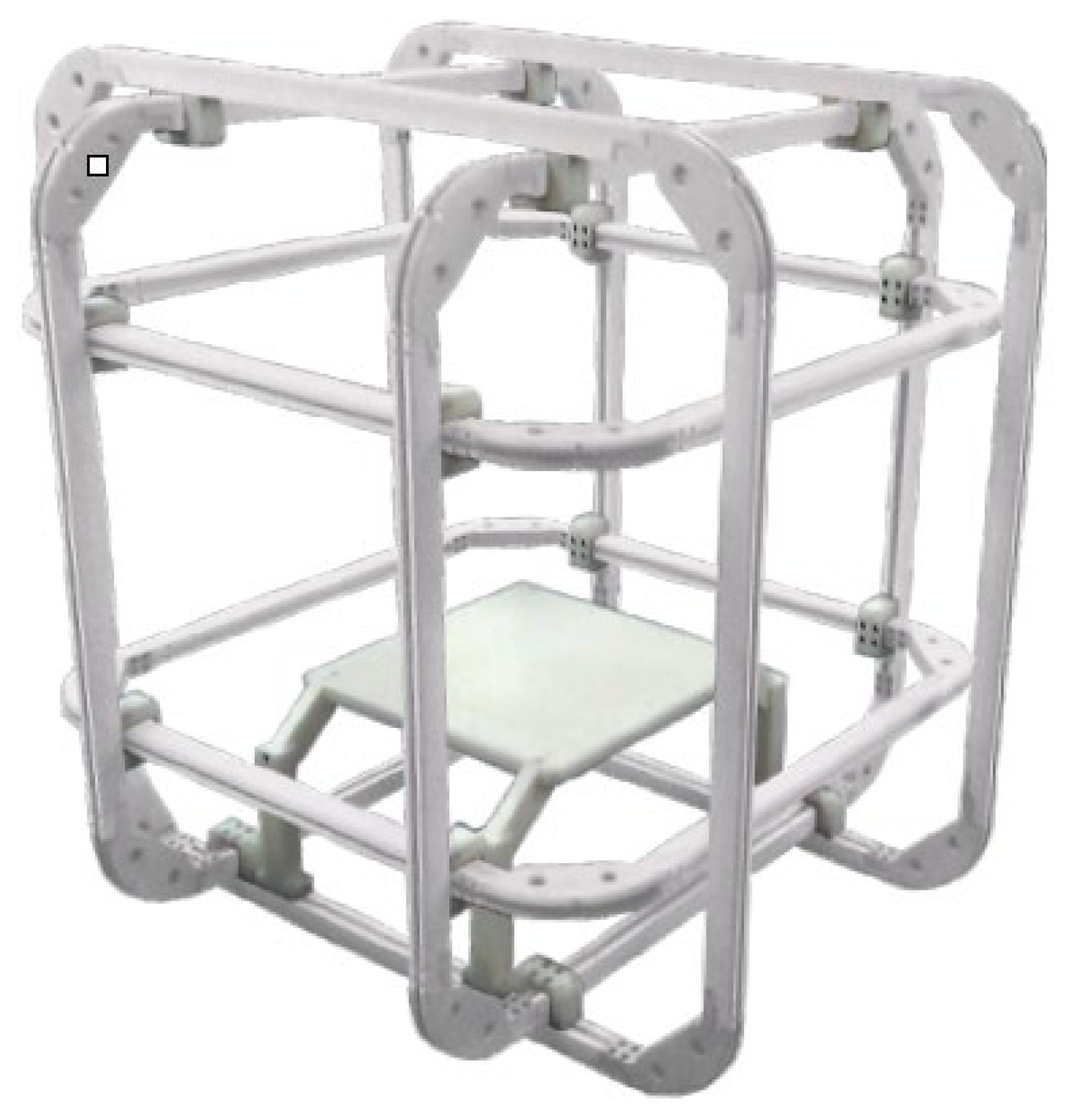
3.1. Three-Dimensional Helmholtz Coil System

The three coils of the system are composed of diameters of ~1 m. They are supplied with a power amplifier and a control unit. Both DC and AC magnetic fields can be generated in any direction (X, Y, Z). The system can serve for calibrating magnetic field sensors or generating a stable and defined magnetic field. All were managed with a National Instruments multifunction card, enabling software control.

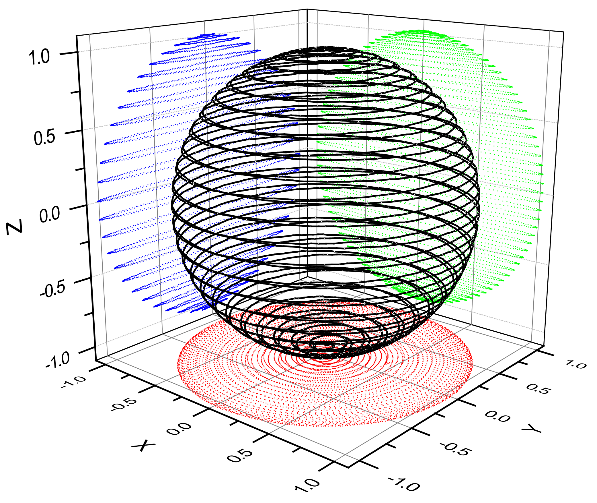
3.2. The Rotating Magnetic Field

To plot the required pattern, we applied a field carried by the three field components ( B x t ,   B y t ,   B z t ). The applied magnetic field functions are given, respectively, as
B x t = B x 0   c o s ω a   t   s i n ω b   t     B y t = B y 0   s i n ω a   t s i n ω b   t       B z t = B z 0   c o s ω b   t                                              
where ω a and ω b are two angular frequencies ( ω a > ω b ) . Their value and ratio are controlled to optimize the plot. The amplitude of the applied field, B 0 , is a constant. It yields B x 2 t + B y 2 t + B y 2 t   = B 0 . So, these parametric equations produce the plot of a sphere in the ideal case when it was sensed by a “true” 3D magnetometer.

3.3. The Sensed Magnetic Field

Experimentally, we expect that our magnetometer is sensitive to its main axis, only, as B x t , for example. In that way, it could be considered as a perfect vector magnetometer. Meanwhile, some discrepancies in its spatial response could be associated with the nature of the sensing element (size, geometry, volume, etc.). Indeed, magnetic sensors are mainly made with magnetic materials. So, its nature or form could imply a spatial shape deformation of the sensed magnetic field.
To summarize, the magnetometer output, up to a certain point, could be proportional to the field components, B x t , B y t , and B z t . Its output voltage might be given by
V o u t t = T x θ , φ   B x t + T y θ , φ   B y t + T z θ , φ   B z t
where T x , T y , and T z are the sensor sensitivity per field direction ( x , y, z). Also, the latter could depend on θ and φ , which are the angular directions of the sensed field given in spherical coordinates. Ideally, T x is a constant and T y and T z are null. For improved comprehension, we provide two examples, hereafter.
Firstly, if we consider T x , T y , and T z  as constant terms, Equation (2) could be reduced. So, the equivalent magnetic sensed field is given by
B S t = B x t + k y x   B y t + k z x   B z t
where k y x = T y / T x and k z x = T z / T x are <<1. Based on these assumptions, we can plot the response of the magnetometer that we named "far-field-pattern". It yields a parametric plot of the projection of the sensed field modulus, B S t , it follows the angular spatial direction of the applied field. It yields three main components given, as far-field pattern (FFP), by
F F P x t = B S t   C o s ω a   t   S i n ω b   t F F P y t = B S t   S i n ω a   t S i n ω b   t     F F P z t = B S t C o s ω b   t                                           ,
respectively. A simulation of this behavior is given in Figure 3a. It shows the ideal and non-ideal response of a vector magnetometer, and blue and red curves, respectively. We can observe a rotation of the main sensitivity axis associated with this imperfection, which we named the “common mode effect”.
To improve the analysis, we notice that all given curves are normalized by the amplitude of the applied field, B 0 . Up to a certain point, a 3D rotation matrix could be associated with this effect and used to correct or compensate for this behavior. Taking into account the assumptions, the difference between an ideal and non-ideal response is given in Figure 3b. It shows the variability of the error versus the applied field angular directions.
Secondly, if we consider T y and T z null, we have only taken account of T x  dependence versus the angular direction of the sensed field. To exemplify, a 2D modeling of one sensor response is detailed hereafter. Ideally, a vector magnetometer sensitivity has a C o s [ θ ] dependence. It yields a parametric plot of T x θ . In 2D, its coordinates are given by 0.5   T x 0 1 + C o s 2 θ , S i n ( 2   θ )   S i g n ( c o s θ )   . It corresponds to a two-lob circular response as given by the blue curve in Figure 4a.
Meanwhile, if we consider an irregular dependence of T x θ , as given by 0.5   T x 0 1 + C o s 2 θ , k 1 S i n 2 θ S i g n c o s θ , as an example, the shape of the parametric plot could change, notably, as exemplified by the orange curve in Figure 4a.
With two orthogonally similar sensors having a response detailed in Figure 4a, Figure 4b gives the angular dependence of the normalized ideal (blue curve) and non-ideal sensor sensitivity (red curve) versus θ .
This analysis can be extended in 3D by including both examples and more complex sensor responses.

4. Discussion

Based on the previous description, we qualify our magnetometers. The amplitude of the applied magnetic field and the angular frequencies ( ω a ,   ω b ) are 10 µT, 2 π rad/s, and 2 π 0.1 rad/s, respectively. All sensor output voltages are acquired by using a homemade 24-bit ADC board. The sampling frequency is 717 Hz. The data acquisition system is managed by a laptop. The latter acquires data for postprocessing. A global view of the setup is given in Figure 5.

Far-Field Pattern

To simultaneously qualify the setup and our GMI magnetometer, a 3D fluxgate magnetometer is used, firstly, to sense the applied field. The experimental normalized response of the three-axis fluxgate is given in Figure 6.
As expected, the 3D fluxgate far-field pattern response is quasi-ideal and looks like a sphere. In the same way, after aligning the GMI magnetometer to the z-axis, we have observed its normalized response. The latter is given in Figure 7. Up to a certain point, the latter corresponds to a true vector magnetometer.
To quantify the measurement, it was possible to evaluate the uncertainties or precision of this measurement based on the intrinsic limitations of our setup. It aims to plot the errors on the sensed field associated with the far-field pattern. Here, we simply subtract the ideal pattern from the normalized measurement response. Notice that both are very similar. The result of this subtraction is given in Figure 8. It shows an observable error lower than ±0.5%.

5. Conclusions

To conclude, we have studied and analyzed the far-field pattern and angular sensitivity dependence of a GMI vector magnetometer and showed its excellent directivity. Our GMI magnetometer can be seen as a quasi-perfect vector sensor. We evaluated the error of axis sensitivity lower than 0.5%. Notice that the given results are limited, certainly, by the environmental noise in the present results (cf. dots spatial distributions in Figure 6). Furthermore, the angular error can be assessed. The development opens the doors to the development of three-axis magnetic field magnetometers having excellent directivity for far magnetic field source detection. Certainly, future enhancements should focus on refining metrological analysis to expand the approach for error localization in source identification, considering the acquired far-field pattern.

Funding

This research received no external funding.

Institutional Review Board Statement

Not applicable.

Informed Consent Statement

Not applicable.

Data Availability Statement

Data are contained within the article.

Conflicts of Interest

The authors declare no conflicts of interest.

References

  1. Ripka, P. Review of fluxgate sensors. Sens. Actuators A 1992, 33, 29–141. [Google Scholar] [CrossRef]
  2. Mohri, K.; Uchiyama, T.; Panina, L.V.; Yamamoto, M.; Bushida, K. Recent Advances of Amorphous Wire CMOS IC Magneto-Impedance Sensors: Innovative High-Performance Micromagnetic Sensor Chip. J. Sens. 2015, 2015, 718069. [Google Scholar] [CrossRef]
  3. Murata, N.; Karo, H.; Sasada, I. Fundamental mode orthogonal fluxgate magnetometer applicable for measurements of DC and low-frequency magnetic fields. IEEE Sens. J. 2018, 99, 2705–2712. [Google Scholar] [CrossRef]
  4. Knobel, M.; Vázquez, M.; Kraus, L. Giant magnetoimpedance. In Handbook of Magnetic Materials; Buschow, K.H.J., Ed.; Elsevier: Amsterdam, The Netherlands, 2003; Volume 15, pp. 497–563. [Google Scholar]
  5. Fodil, K.; Denoual, M.; Dolabdjian, C. Experimental and Analytical Investigation of a new 2D Magnetic Magnetic Imaging Method using magnetic nanoparticules. IEEE Trans. Magn. 2016, 52, 6500109. [Google Scholar] [CrossRef]
  6. Clem, T.R.; Kelis, G.J.; Lathrop, J.D.; Overway, D.J.; Wynn, W.M. Superconducting Magnetic Gradiometers for Mobile Applications with an Emphasis on Ordnance Detection. In SQUID Sensor: Fundamentals, Fabrication and Applications; Weinstock, H., Ed.; Kluwer Academic Publishers: Dordrecht, The Netherlands, 1996; Volume 329. [Google Scholar] [CrossRef]
  7. Sheinker, A.; Frumkis, L.; Ginzburg, B.; Salomonski, N.; Kaplan, B.-Z. Magnetic Anomaly Detection Using a Three-Axis Magnetometer. IEEE Trans. Magn. 2009, 45, 160–167. [Google Scholar] [CrossRef]
  8. Zhao, Y.; Zhang, J.H.; Li, J.H.; Liu, S.; Miao, P.X.; Shi, Y.C.; Zhao, E.M. A brief review of magnetic anomaly detection. Meas. Sci. Technol. 2021, 32, 042002. [Google Scholar] [CrossRef]
  9. Dolabdjian, C.; Cordier, C. Analysis by systemic approach of magnetic dipole source location performances by using an IoT software gradiometer head. IEEE Sens. J. 2022, 22, 7709–7716. [Google Scholar] [CrossRef]
  10. Dufay, B.; Saez, S.; Dolabdjian, C.P.; Yelon, A.; Menard, D. Characterization of an optimized off-diagonal GMI-based magnetometer. IEEE Sens. J. 2013, 13, 379–388. [Google Scholar] [CrossRef]
  11. Esper, A.; Dufay, B.; Saez, S.; Dolabdjian, C. Theoretical and Experimental Investigation of Temperature-Compensated Off-Diagonal GMI Magnetometer and Its Long-Term Stability. IEEE Sens. J. 2020, 20, 9046–9055. [Google Scholar] [CrossRef]
Figure 1. View of (a) the GMI sensor mount with its pick coil and (b) its conditioning electronic boards.
Magnetism 04 00004 g001
Figure 2. View of the three-axis Helmholtz coil system. In its center, the homogenous induced magnetic field covers a volume of around 25 × 25 × 25 cm3. The system is controlled with a desktop, which manages each field axis in terms of shape, frequency, and amplitude, independently.
Magnetism 04 00004 g002
Figure 3. (a) Normalized ideal far-field pattern (blue curve) compared to the non-ideal far-field pattern response (red curve) having k y x = k z x = 0.2 . (b) The orange curve shows the difference between both.
Magnetism 04 00004 g003
Figure 4. (a) Normalized ideal T x θ 2D dependence (blue curve) compared to a non-ideal T x θ dependence (orange curve). (b) For two identical magnetometers placed orthogonally, the blue and orange curves give a circular response in the ideal case ( T θ = 1 ) and a distorted response in a non-ideal case T x θ = 0.5   T x 0 1 + C o s 2 θ , k 1 S i n 2 θ S i g n c o s θ , respectively.
Magnetism 04 00004 g004
Figure 5. Global view of the experimental setup.
Magnetism 04 00004 g005
Figure 6. Experimental three-axis fluxgate directional far-field patterns (or angular sensitivity dependence) versus an applied rotating magnetic field having an amplitude, B 0 , of 10 µT. Notice that the curve is normalized in amplitude by B 0 . Blue, red and green curves highlight the projection of the magnetic sensor response in each plane (z, y), (x, y) and (z, y), respectively.
Magnetism 04 00004 g006
Figure 7. Experimental GMI directional far-field patterns or angular dependence of their sensitivity versus an applied rotating magnetic field having an amplitude of 10 µT. Notice that the curve is normalized in amplitude by B 0 . Blue, red and green curves highlight the projection of the magnetic sensor response in each plane (z, y), (x, y) and (z, y), respectively.
Magnetism 04 00004 g007
Figure 8. Experimental GMI magnetometer error associated to the far-field pattern given in Figure 7. Blue, red and green dots highlight the projection of the magnetic sensor errors in each plane (z, y), (x, y) and (z, y), respectively.
Magnetism 04 00004 g008
Table 1. Main magnetometer characteristics.
Characteristics Units
Sensitivity54,000V/T
White noise level15pT/√Hz
Bandwidth30,000Hz
1/f noise corner5Hz
Dynamic range±60µT
Long-term stability>5nT/h
Disclaimer/Publisher’s Note: The statements, opinions and data contained in all publications are solely those of the individual author(s) and contributor(s) and not of MDPI and/or the editor(s). MDPI and/or the editor(s) disclaim responsibility for any injury to people or property resulting from any ideas, methods, instructions or products referred to in the content.

