Analysis of Vector Network Analyzer Thermal Drift Error

Abstract

Ensuring a high accuracy when measuring the parameters of devices under testing is an important task when conducting research in the terahertz-frequency range. The purpose of this paper is a practical study of the thermal drift errors of a vector network analyzer using low-terahertz-frequency extender modules. For this, the change in the measurement error, which is a function of time, was analysed using system, based on Keysight N5247B vector network analyzer and covering the frequency ranges of 220–330 GHz, 500–750 GHz, and 750–1100 GHz. The results of our experiment showed that the measurement error decreased rapidly during the first half hour of warm-up and stabilized by 3 h after turning on the equipment. These results allow for an estimation of the necessary warm-up time depending on the requirements for the measurement’s accuracy. This makes it possible to optimize the experiment and reduce its duration.

1. Introduction

Ensuring a high accuracy of scattering parameters (S-parameters) measurement using a vector network analyzer (VNA) is an important task when conducting research in the low-terahertz (low THz)-frequency band. When making measurements, we must always consider imperfections that exist in even the highest-quality test equipment and can cause less-than-ideal measurement results. Some factors that contribute to measurement errors are repeatable and predictable dependent on time and temperature and can be removed, while other errors are random and cannot be removed.

VNA measures the amplitude and phase of a signal interacting with a device-under-test (DUT); it operates in the frequency domain, providing frequency-dependent data [1]. VNAs working at millimeter-wave and low THz frequencies are usually equipped with frequency extender modules fitted with standardized rectangular metal waveguides. The measurement quantities are the magnitude and phase of the propagating signals incident on and scattered from each port. The VNA forms ratios of these quantities to present S-parameters for the DUT.

The typical VNA architecture necessarily introduces several systematic errors. These are inevitable due to the possibility of different port impedances, measurement signal path losses, phase shifts, internal reflections, and factors, such as an imbalance in the directional couplers that form the test/stimulus ratios [1,2]. However, for these errors, the linearity condition can be accepted, and they can be corrected or reduced to acceptable values using the calibration procedure.

Random errors are inherently unpredictable, so they cannot be removed by calibration. The main contributors to random errors are instrument noise (for example, sampler noise and the IF noise floor), switch repeatability and connector repeatability. When using VNAs, noise errors can often be reduced by increasing the source power, narrowing the IF bandwidth, or using trace averaging over multiple sweeps. The proper care and handling of the RF connectors in the measurement system can minimize connector repeatability errors.

Drift errors occur when a test system’s performance changes after a calibration has been performed. These errors are caused primarily by temperature variation and can be removed by additional calibration. The rate of drift determines how frequently additional calibrations are needed. Establishing a test environment with a stable ambient temperature usually minimizes drift errors. Allowing equipment to warm up and stabilize before calibration and properly ventilating equipment helps reduce drift errors. A summary of the VNA errors is given in

Table 1. VNA errors.

Error Type	Systematic	Random	Drift
Cause of measurement error	Imperfections in the test equipment and test setup	Instrument noise and connector repeatability	Temperature variation
Error compensation technique	Calibration	Increasing source power, narrowing the IF bandwidth or trace averaging. Proper care and handling of the RF connectors	Additional calibration. Stable ambient temperature

. To calculate the uncertainties of VNA measurements, including drift of switch and error terms of the calibration, the METAS VNA Tools [3] can be used.

VNA manufacturers’ usual recommendation is to give the instrument from one to two hours to warm up [4,5]. In this paper, the dependence of the measurement accuracy associated with the temperature drift error depending on the warm-up time of the device is given. Thus, in [5], it was stated that the thermal drift of the VNA error was less than 0.02 dB after a 20 min warm-up time and less than 0.01 dB after a 1 h warm-up time. However, the results presented refer to the device without frequency extension modules, which, due to the design features that will be discussed later in this paper, are more susceptible to the influence of temperature drift.

In the available publications, we did not find an analysis of thermal drift errors of VNAs equipped with frequency extension modules. When conducting practical experiments using VNA, it is important to know the dependence of the measurement error on the time elapsed from the moment the device is turned on. It may be that, for low accuracy requirements, half an hour is sufficient, but for higher accuracy requirements, the device will need to warm up for two hours. A common approach to ensure low-temperature drift errors is to keep the VNA on permanently, but this mode is possible only if the measuring setup is unchanged. When operating the VNA in a university, it is often necessary to change the frequency modules and reconfigure the measuring layout, which leads to the need to turn off the device.

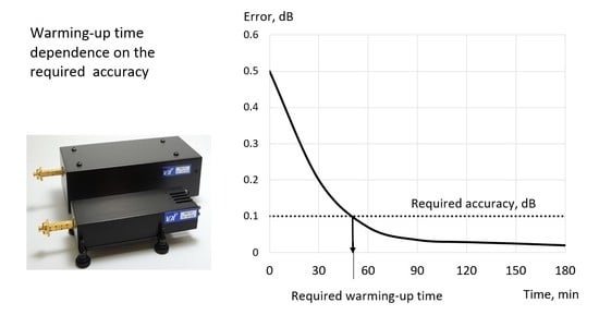
This paper’s purpose is a practical study of the influence of the warm-up time and, accordingly, the VNA temperature on the thermal drift errors. The results obtained make it possible to estimate the necessary time for warming up the VNA depending on the measurement requirements, making it possible to reduce the experiment duration without losing accuracy. The purpose of the warm-up is to achieve the thermal equilibrium of the system; therefore, the properties of the DUT will influence this process. If a very large DUT is used, the required warm-up time may increase. Nevertheless, the results obtained in the research can serve as a guide in most practical cases.

The remainder of this paper is organized as follows. In Section 2, the VNA thermal drift errors and methods of their measurement are discussed. The experimental results are presented in Section 3, and their discussion is detailed in Section 4. Finally, the conclusions are formulated in Section 5.

2. Measurement of Thermal Drift Errors

2.1. Thermal Drift Errors

The thermal drift cause is either the measurement signal path or the electronic circuits within the VNA and the extender heads. Temperature changes will produce small changes in physical dimensions through linear expansion. These changes can be significant at submillimeter-wave and THz frequencies [2]. Small changes in signal path dimensions due to thermal expansion can lead to noticeable differences, particularly in phase. Let us consider an example. The coefficient of the linear thermal expansion of copper is 16.6 ppm/°C. Suppose that the waveguides used to connect the extender heads to the DUT are 10 cm long. Then, while changing the temperature by 5 °C, the waveguide length will increase by 8.5 μm, which at a frequency of 1 THz, will lead to a phase shift of 9.2°.

The flexible cables used to connect the extender heads to the VNA are exposed to ambient thermal fluctuation. Nonetheless, the effect of changing their length will not be as significant as that for waveguides and extender modules. Indeed, the signal frequency in these cables usually does not exceed 20 GHz, and when the temperature changes at 5 °C, as in the example considered above, the phase shift will not exceed 2° at a length of 1 m.

As we already mentioned, the effects of thermal drift can be reduced by allowing the VNA equipment to thermally stabilize before use. In practice, this means that the equipment should be switched on for several hours before calibration and measurements take place. As indicated in [4], directly after power-up the cold instrument should be allowed to warm up for approximately an hour to attain thermal equilibrium. The manufacturer recommends giving the VNA at least two hours to warm up if a higher accuracy is required. Failing to carry this out will result in a noticeable “drift” in the measurement trace, usually if the laboratory temperature is cool. This is because the internal temperature in the VNA itself and the extender heads will considerably increase during the first two hours.

It is also essential to maintain a stable ambient temperature. Ideally, the network analyzer should be operated in a temperature-controlled laboratory to minimize the possibility of thermal fluctuation to these parts of the signal path. For Keysight VNAs, calibrated system performance is within the specifications if the ambient temperature at the time of the measurement is within 1 °C of the temperature at the calibration time [4].

As we can see, the recommendations of equipment manufacturers lie in a wide range. Therefore, to ensure the quality of measurements, we need to know the warm-up time’s sufficiency. This is especially important when using millimeter-wave or THz extender heads. This study aims to address the accuracy of measuring DUT parameters in the millimeter and low-THz-frequency ranges depending on the warm-up time.

2.2. Experiment Setup

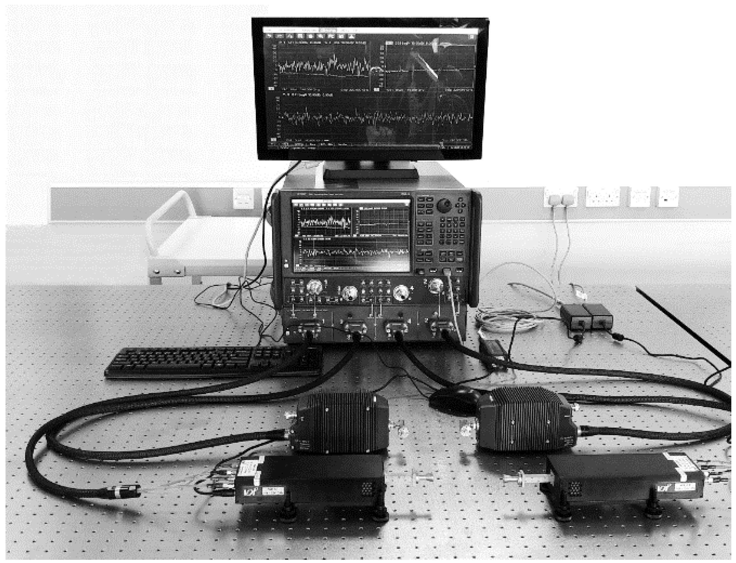
We used the Terahertz measurement facility’s services at the University of Birmingham [6]. The centerpiece of the facility is the Keysight N5247B vector network analyzer (Figure 1), manufactured by Keysight Technologies (Santa Rosa, CA, USA) [7].

The VNA can measure the full two-port scattering parameters in the frequency range up to 1.1 THz using the frequency-converter units. We measured the thermal drift errors using the following three-vector network analyzer frequency extension modules manufactured by Virginia Diodes Inc. (VDI, Charlottesville, VA, USA): WR3.4, WR1.5, and WR1.0 [8]. The choice of these modules was due to the desire to cover a wide frequency range and their design differences. The WR3.4 module is made in a mini-sized enclosure, and the WR1.5 and WR1.0 modules are made in a standard size enclosure [9]. We wanted to find out if these design features lead to differences in the values of temperature drift. The characteristics of the modules are presented in

Table 2. Characteristics of the frequency extension modules.

Parameter	WR3.4	WR1.5	WR1.0
Frequency coverage, GHz	220–330	500–750	750–1100
Dynamic range, dB	115	100	65
Magnitude stability, ±dB	0.3	0.4	0.5
Phase stability, ±degrees	6	4	6
Test port power, dBm	1	−25	−30

.

Stability is specified for 1 h after system warm-up in a stable environment with ideal cables. The recommended operating temperature range of the modules is from 20 °C to 30 °C. The modules are equipped with waveguides with UG-387/U-M flanges [2]. Calibrations and measurements were made without the use of internal flange pins, in accordance with the manufacturer’s standard recommendations.

The THz measurement facility was not equipped with a temperature control; however, it was possible to maintain a stable ambient temperature within the recommended operating temperature limits 20–30 °C. The temperature variations during the measurement did not exceed 0.5 °C, and in the corresponding section, we will provide detailed temperature data. On the eve of the measurement, the device was calibrated using the appropriate standard calibration kit; the cables and modules did not change their position before and during the measurement. The measurements were made with a short-circuited waveguide from the calibration kit.

2.3. Calculation of Measurement Error

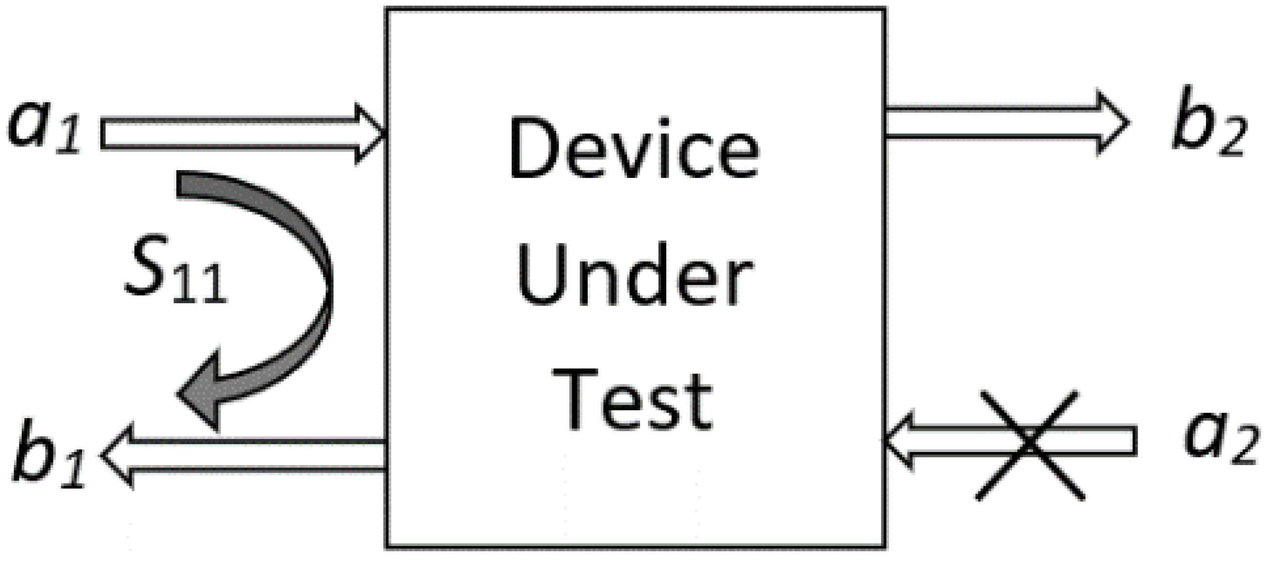
VNA measures scattering or S-parameters, which are complex matrix elements that show reflection/transmission characteristics (amplitude and phase) in the frequency domain. The ratio of received power to the transmitted power can be expressed through the magnitude of the input port voltage reflection coefficient S₁₁ [1]:

$$S_{11}=\frac{b_1}{a_1} \mathrm{when} a_2=0,$$

(1)

where a₁ and a₂ are incident power waves at ports 1 and 2, respectively, and b₁ is reflected wave for port 1 (see Figure 2). In a perfect termination case, the magnitudes of b₁ and a₁ are equal, and the magnitude |S₁₁|, expressed in dB, should be zero. In real conditions, each measurement of |S₁₁| will always be slightly greater or less than zero due to random errors in the measurement process. In our experiment, we used the magnitude and phase of this deviation to estimate the measurement error. Since reflection coefficient S₁₁ is a complex quantity, it is characterized by the complex value’s real and imaginary components or its magnitude and phase.

The entire frequency range from f₁ to f₂ is presented in the form of n discrete frequencies with a step of:

$$f_s=\frac{f_2-f_1}{n-1}.$$

(2)

Since we wished to estimate the temperature drift over the entire frequency range, at each time moment, we measured S₁₁ for n discrete frequencies, which allowed us to statistically draw valid conclusions about the measurement accuracy. The measurements continued for three hours with an interval of t_s = 10 min; therefore, the total number of measurements m was 3 × 60/10 + 1 = 19.

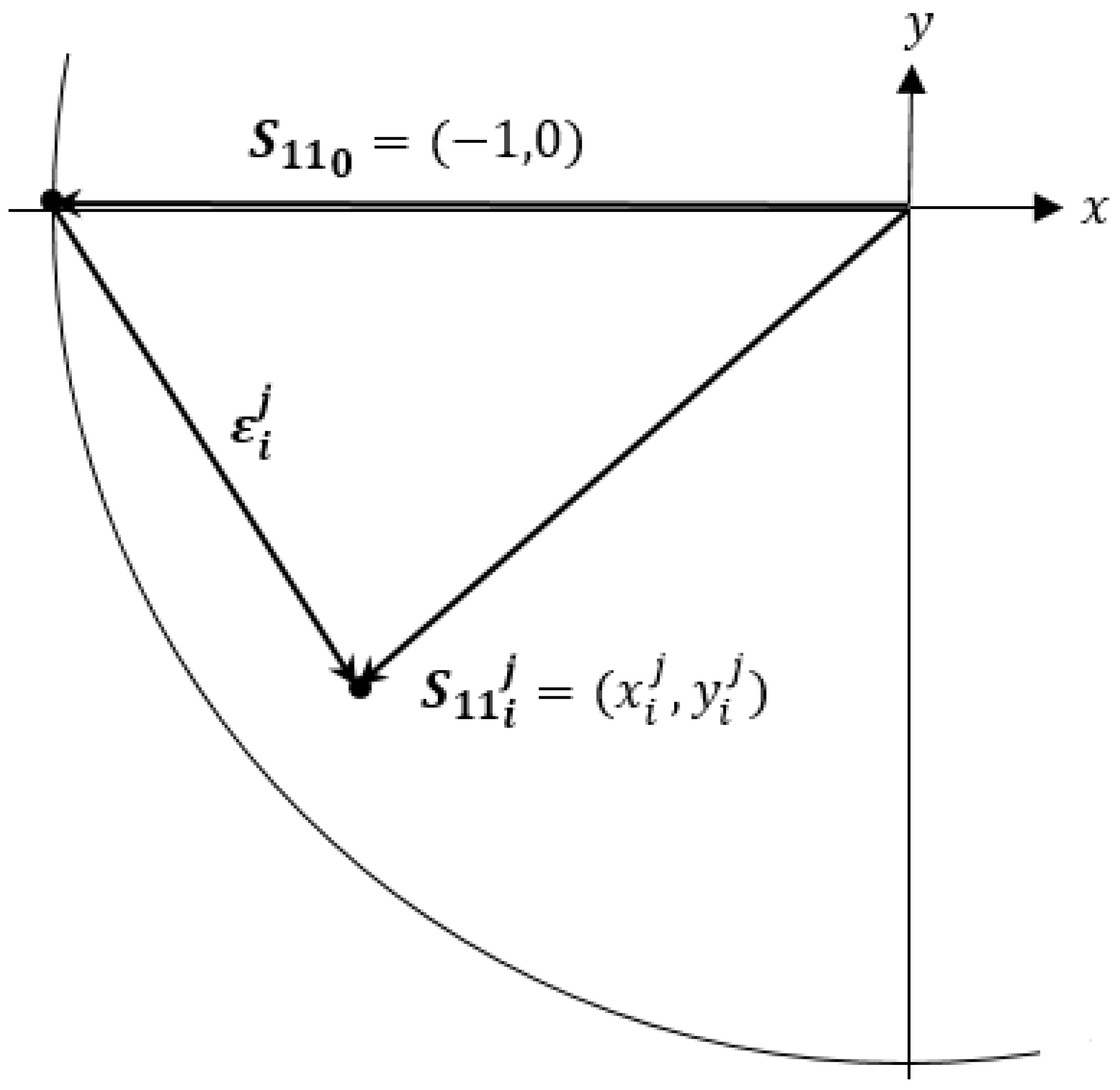
Figure 3 explains the process of calculating a measurement error for S₁₁ coefficient with coordinates in the complex plain $(x_i^j, y_i^j)$. Hereinafter, the superscript j corresponds to the measurement serial number. It varies from 1 to m, and the subscript i corresponds to the number of the discrete frequencies and varies from 1 to n. Coordinates (−1, 0) in the complex plane correspond to a zero measurement error of coefficient S₁₁. The zero error corresponds to the vector ${\mathit{S}}_{{\mathbf{11}}_{\mathbf{0}}}$, and each current measurement corresponds to the vector ${{\mathit{S}}_{\mathbf{11}}}_{\mathit{i}}^{\mathit{j}}$.

The error vector for the current measurement that is, at time $t=j{t}_s$ and at frequency $f=i{f}_s$, can be calculated as the difference between vectors:

$${\mathit{\epsilon }}_{\mathit{i}}^{\mathit{j}}={\mathit{S}}_{\mathbf{11}}{}_{\mathit{i}}^{\mathit{j}}-{\mathit{S}}_{{\mathbf{11}}_{\mathbf{0}}}.$$

(3)

We are interested in how the error, averaged over the entire frequency range, changes over time. To determine the average magnitude of the measurement error vector ${\mathit{\epsilon }}^{\mathit{j}}$ at the time moment j, we must average this magnitude over all n frequencies:

$$\langle \left|{\mathit{\epsilon }}^{\mathit{j}}\right|\rangle =\frac{1}{n}{\displaystyle \sum }_{i=1}^n\left|{\mathit{\epsilon }}_{\mathit{i}}^{\mathit{j}}\right|.$$

(4)

However, in most cases, this averaging can lead to the appearance of a systematic error [10]. For example, if the average value of the complex vector ${\mathit{\epsilon }}_{\mathit{i}}^{\mathit{j}}$ is equal to zero ($\langle {\mathit{\epsilon }}^{\mathit{j}}\rangle =0$), then each individual measured value of the magnitude is nonzero, and averaging the magnitude would give us a value that differs from the true value ($\langle \left|{\mathit{\epsilon }}^{\mathit{j}}\right|\rangle >0$).

Therefore, in this paper, we expressed all complex-valued measurements in real and imaginary components before applying statistical techniques to analyze complex-valued data. The complex quantity ${\mathit{\epsilon }}^{\mathit{j}}$ represents an error at the time moment of jt_s, averaged over all n frequencies:

$${\mathit{\epsilon }}^{\mathit{j}}=\frac{1}{n}{{\displaystyle \sum }}_{i=1}^n{\mathit{\epsilon }}_{\mathit{i}}^{\mathit{j}}.$$

(5)

The real component of ${\mathit{\epsilon }}^{\mathit{j}}$ can be expressed as:

$$Re\left({\mathit{\epsilon }}^{\mathit{j}}\right)=\frac{1}{n}{{\displaystyle \sum }}_{i=1}^{n}Re\left({\mathit{\epsilon }}_{\mathit{i}}^{\mathit{j}}\right).$$

(6)

The mean of the imaginary component of the complex quantity ${\mathit{\epsilon }}^{\mathit{j}}$ can be expressed as:

$$Im\left({\mathit{\epsilon }}^{\mathit{j}}\right)=\frac{1}{n}{{\displaystyle \sum }}_{i=1}^{n}Im\left({\mathit{\epsilon }}_{\mathit{i}}^{\mathit{j}}\right).$$

(7)

The magnitude of the complex quantity ${\mathit{\epsilon }}^{\mathit{j}}=Re\left({\mathit{\epsilon }}^{\mathit{j}}\right)+iIm\left({\mathit{\epsilon }}^{\mathit{j}}\right)$ is:

$$\left|{\mathit{\epsilon }}^{\mathit{j}}\right|=\sqrt{{\left[Re\left({\mathit{\epsilon }}^{\mathit{j}}\right)\right]}^2+{\left[Im\left({\mathit{\epsilon }}^{\mathit{j}}\right)\right]}^2}.$$

(8)

The standard deviation of ${\mathit{\epsilon }}^{\mathit{j}}$ is equal to the sum of the standard deviations of its real and imaginary parts [11]:

$$D\left({\mathit{\epsilon }}^{\mathit{j}}\right)=D\left[Re\left({\mathit{\epsilon }}^{\mathit{j}}\right)\right]+D\left[Im\left({\mathit{\epsilon }}^{\mathit{j}}\right)\right].$$

(9)

The phase θ of the complex quantity ${\mathit{\epsilon }}^{\mathit{j}}$ can be found from:

$$tan\theta =Im\left({\mathit{\epsilon }}^{\mathit{j}}\right)/Re\left({\mathit{\epsilon }}^j\right).$$

(10)

In the next section, we present the results of temperature drift measurements based on this approach.

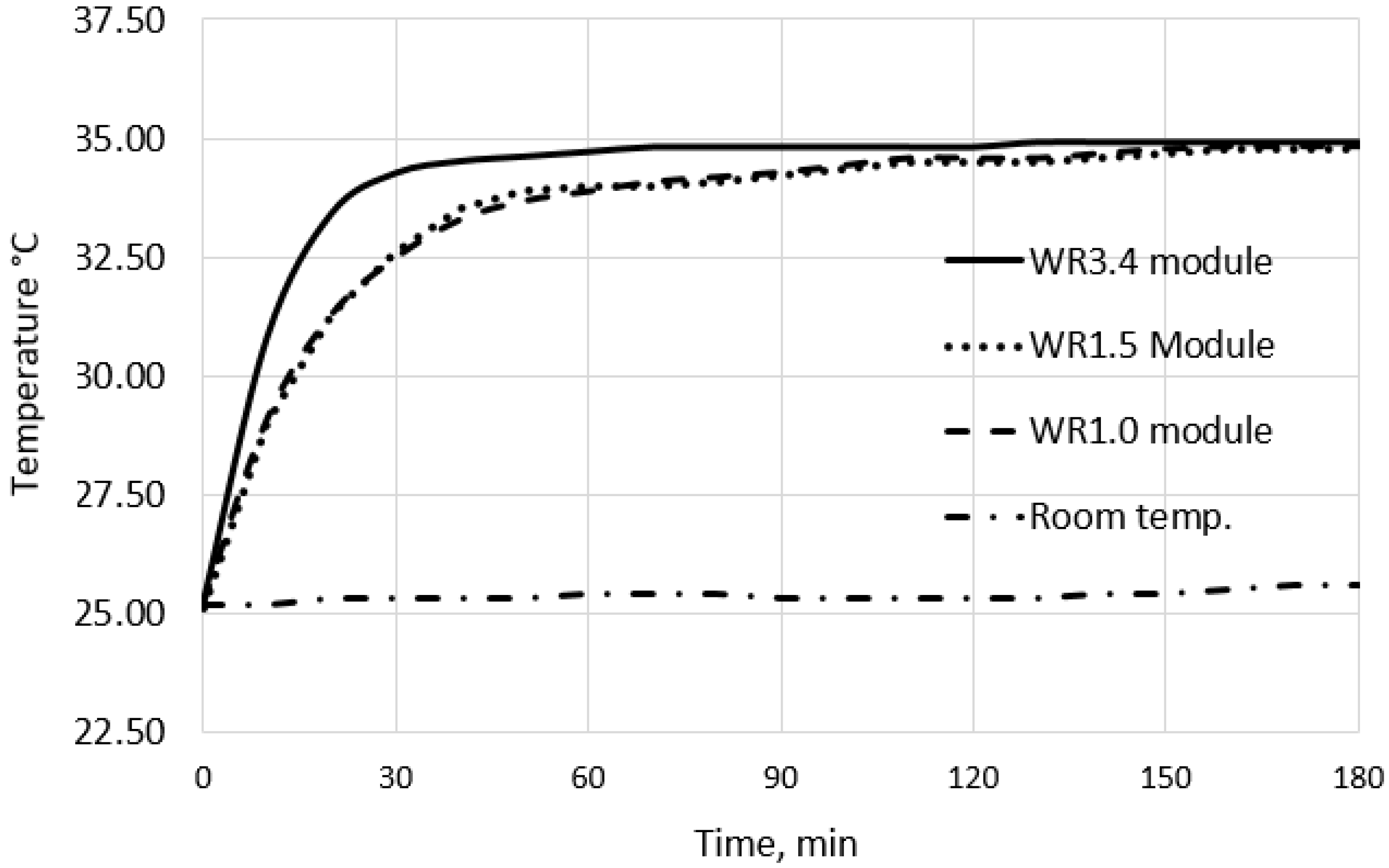
2.4. Ambient and Device Temperature

The results of temperature measurements using Duratool Infrared Thermometer D03308 are presented in Figure 4. The room temperature is given for measurement with WR3.4 module; when using WR1.0 and WR1.5 modules, it was not significantly different (±0.2 °C) from that shown in Figure 3. In the considered example, over three hours of the experiment, it increased from 25.2 °C to 25.6 °C; these temperature variations are within the equipment manufacturer’s recommendations.

For definiteness, we measured the temperature on the flange that connects the waveguide to the extender head. This temperature does not give the exact value of the temperature of the VNA or frequency extender head. Nonetheless, since we are interested in the temperature change, this measurement is adequate for the experiment.

For three hours, the compact WR3.4 module temperature measured on the waveguide flange increased from 25.2 °C to 34.9 °C, while by the end of the first hour, it was 34.7 °C and almost reached a stable temperature exceeding the room temperature by 9.3–9.5 °C, and this difference remained almost unchanged. Fluctuations within ±0.1 °C can be attributed to the thermometer resolution since its minimum display scale value is 0.1 °C. The temperature of the full-size WR1.5 and WR1.0 modules grew more slowly and only after three hours their temperature became 34.9 °C, the same as that of the WR3.4 module.

3. Results

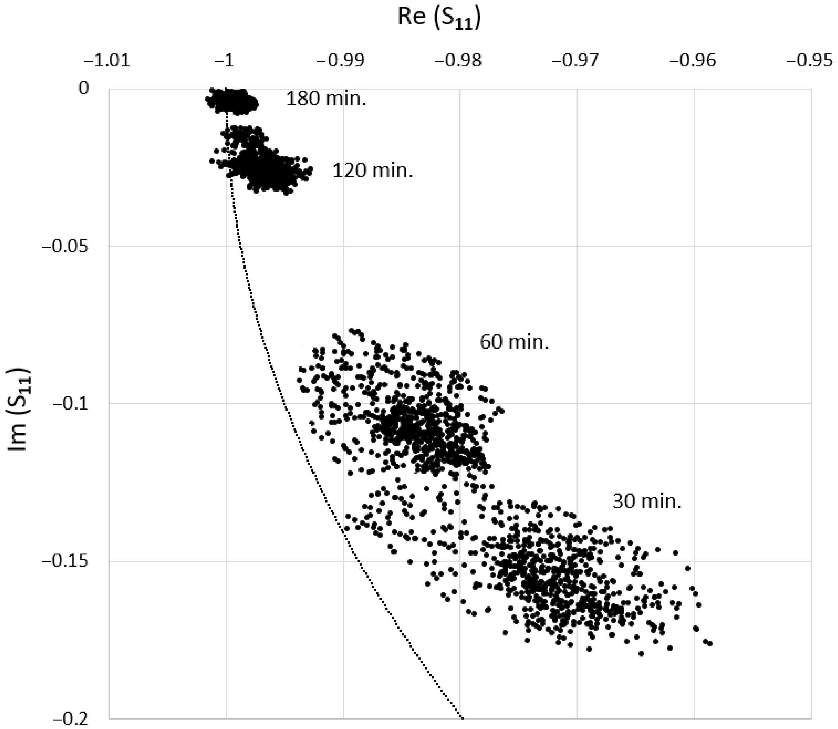
To understand how the measurement error changes over time, it is convenient to present the measurement results in a scatter plot on the complex plane. In Figure 5, the distribution of measured S₁₁ is shown for four measurements made after 30 min, 60 min, 120 min, and 180 min from the beginning of the experiment with WR3.4 module. Each point in the figure represents the S₁₁ coefficient for one of the frequencies. The entire measurement range from 220 to 300 GHz was presented in 801 discrete frequencies with a step of 137.5 MHz as determined by (2).

As we have already noted, a zero error corresponds to ${\mathit{S}}_{{\mathbf{11}}_{\mathbf{0}}}$= (−1, 0). In Figure 4, the line represents a sector of a circle with the magnitude |S₁₁| = 1. The distance of each measured value of S₁₁ from this circle corresponds to a measurement error of this coefficient’s magnitude. As can be seen from the figure, with increasing time, this error decreases. The phase measurement error corresponds to the angle of the measured S₁₁ to the axis $x=Re\left(S_{11}\right).$ It decreases as the device warms up. From Figure 5 we see that a standard deviation of the measurement error decreases over time; it is characterized by the size of the corresponding ellipse of the scatter of the measured values. The scatters vary if different modules are used, but the general patterns remain as shown in Figure 5.

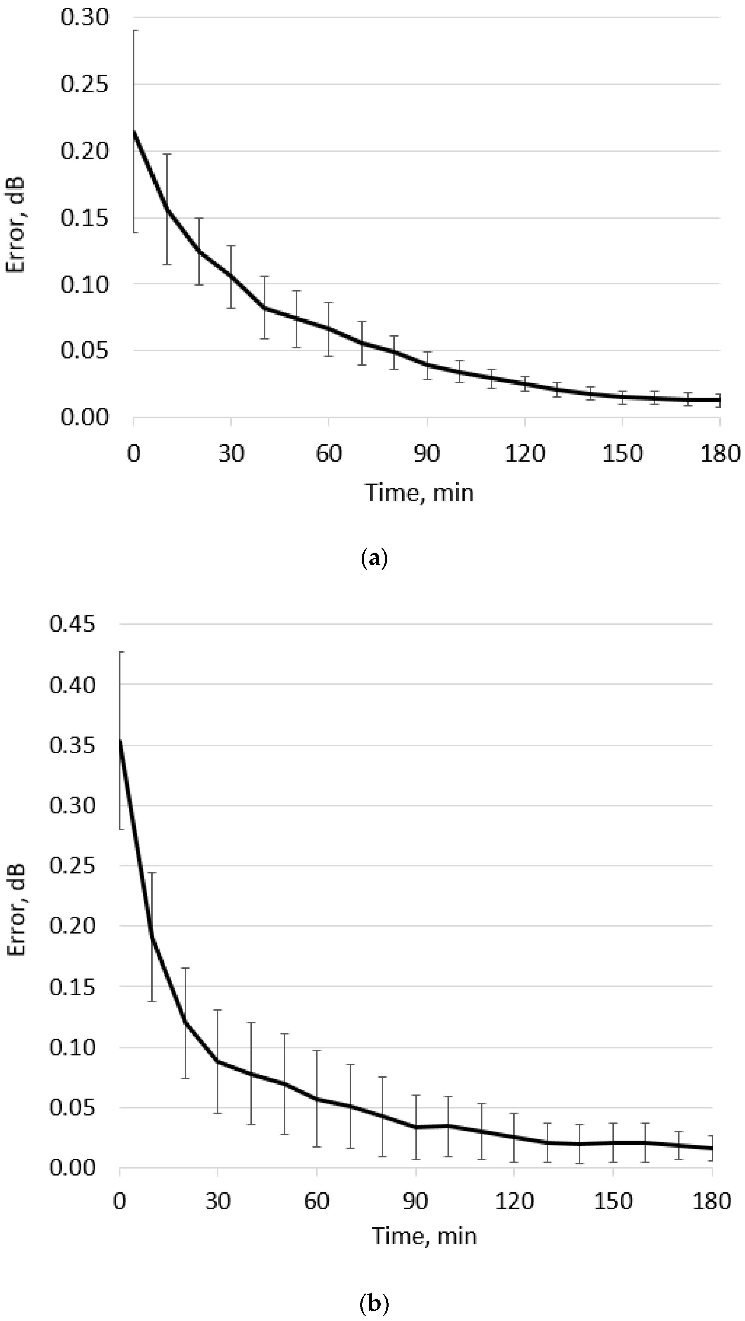
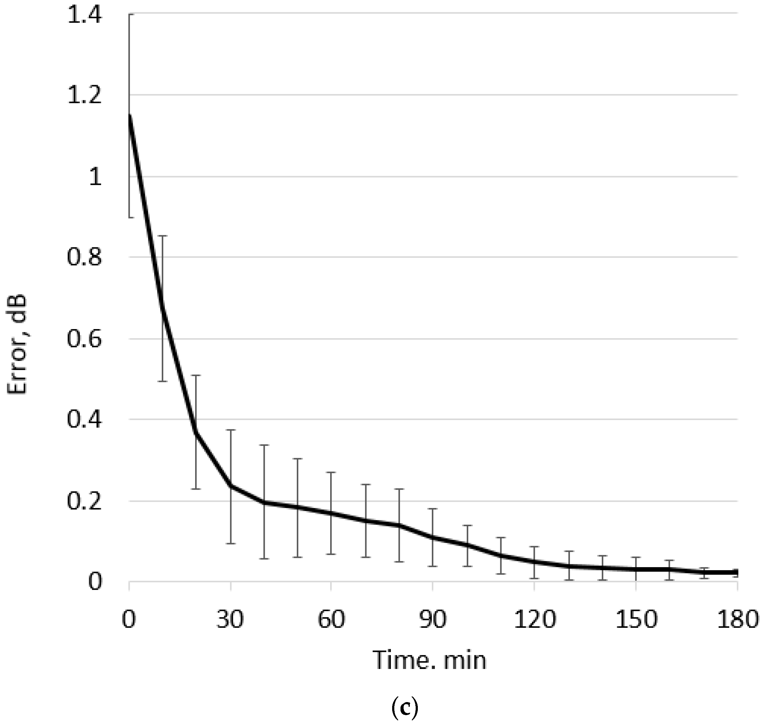
We calculated the magnitude of the measurement error, its standard deviation, and the phase error for all three modules used, depending on the time from the start of the experiment. The graphs for magnitude errors are shown in Figure 6a–c, and numerical results in dB are shown in

Table 3. Magnitude error in dB/phase error in degrees.

Time	WR3.4	WR1.5	WR1.0
30 min.	0.105/6.70°	0.088/2.45°	0.235/2.90°
60 min.	0.066/2.78°	0.057/0.62°	0.171/1.96°
90 min.	0.039/1.62°	0.034/0.47°	0.112/0.29°
120 min.	0.025/0.92°	0.026/0.33°	0.044/0.19°
150 min.	0.015/0.45°	0.020/0.10°	0.030/0.14°
180 min.	0.013/0.12°	0.016/0.03°	0.020/0.09°

. As can be seen from these graphs, the measurement error rapidly decreases within the first 30 min. In the first two cases (WR3.4 and WR1.5), it decreases to about 0.1 dB, and in the third case (WR1.0), it decreases to about 0.2 dB. This reduction in measurement error continues more smoothly until approximately two hours from the start of measurement. During this period, the error becomes 0.025–0.044 dB. In the range from two to three hours, this decrease continues slowly until 0.013–0.020 dB is reached.

The phase error measurements shown in Table 3 demonstrate similar patterns. It should be noted that a significantly larger error was found when using the WR3.4 module. Perhaps this is because the length of the connecting waveguide, in this case, is 10 cm; in higher frequency modules, it is 4 cm. Temperature changes, in this case, have a more significant effect on the phase shift of the signal.

4. Discussion

Thus, we can confirm the equipment manufacturer’s recommendation of the need to warm up the equipment for two hours before the start of experiment. With high requirements for measurement accuracy, this interval should be increased to three hours. The minimum warm-up time for low accuracy requirements is 30 min. The reduction in the measurement error correlates well with the temperature of the modules presented in the graph in Figure 6. It is seen that the maximum temperature change occurs in the first 30 min, and the temperature increases up to 2 h from the start. The highest-frequency module WR1.0 has the most significant measurement error; seemingly, this is due to its design features and technological parameters.

As shown in Table 3, the measurement error remained noticeable even after three hours. This is because the instrument was calibrated on the eve of the measurement and switched off overnight. To achieve maximum accuracy, the VNA must be calibrated when thoroughly warmed. In the experiment, we could not do this because it was the temperature drift error during the warming process that interested us.

5. Conclusions

This work aimed to study the temperature drift error of VNA to determine the optimal warm-up time depending on the requirements for measurement accuracy. For this, we analyzed the change in the measurement error of the S₁₁ coefficient as a function of time using VNA Keysight N5247B with WR3.4, WR1.5, and WR1.0 Low THz frequency extender modules, covering frequency ranges of 220–330 GHz, 500–750 GHz, and 750–1100 GHz. Our results showed that the measurement error decreases rapidly during the first 30 min of equipment warm-up and practically stabilizes by 3 h. The optimal time in our cases is about 2 h. These conclusions should be considered as a guide, since in each case, the temperature drift error will be influenced by factors such as the DUT used and the initial ambient temperature. These and other questions will be explored in the continuation of this research. The results obtained are important in terms of organizing and conducting measurements using VNA.