Article

Experimental Design for Virtual Experiments in Tilted-Wave Interferometry

1
Physikalisch-Technische Bundesanstalt (PTB), Bundesallee 100, 38116 Braunschweig, Germany
2
Physikalisch-Technische Bundesanstalt (PTB), Abbestraße 2-12, 10587 Berlin, Germany
*
Author to whom correspondence should be addressed.
Metrology 2022, 2(1), 84-97; https://doi.org/10.3390/metrology2010006
Submission received: 7 December 2021 / Revised: 17 January 2022 / Accepted: 9 February 2022 / Published: 17 February 2022
(This article belongs to the Special Issue Virtual Measuring Systems and Digital Twins)

Abstract

:
The tilted-wave interferometer (TWI) is a recent and promising technique for optically measuring aspheres and freeform surfaces and combines an elaborate experimental setup with sophisticated data analysis algorithms. There are, however, many parameters that influence its performance, and greater knowledge about the behavior of the TWI is needed before it can be established as a measurement standard. Virtual experiments are an appropriate tool for this purpose, and in this paper we present a digital twin of the TWI that was carefully designed for such experiments. The expensive numerical calculations involved combined with the existence of multiple influencing parameters limit the number of virtual experiments that are feasible, which poses a challenge to researchers. Experimental design is a statistical technique that allows virtual experiments to be planned such as to maximize information gain. We applied experimental design to virtual TWI experiments with the goal of identifying the main sources of uncertainty. The results from this work are presented here.

Graphical Abstract

1. Introduction

Because of their ability to correct optical aberrations using fewer optical elements, aspheric and freeform lenses gained attention as building blocks for compact sophisticated optics [1,2,3]. To enable the fabrication of the highly accurate aspheric surfaces required, accurate measurement systems are a must. The measurement methods suited for this purpose can be divided into two categories: pointwise and areal. The pointwise methods can be further separated into those using tactile probes [4] and optical point sensors [5], whereas areal methods are typically used by interferometric [6,7] or deflectometric [8,9] measurement systems. Pointwise methods are highly adaptable since they are often not subject to any fundamental limitations with respect to the surface forms they can measure. Long measurement times, however, limit the applicability of these procedures for measurements during production, or lead to measurement results with lower lateral resolution. In contrast, areal measuring methods are usually associated with short measurement times (good for production line integration) and high lateral resolution, but might be limited in their range of measurable surfaces. Common interferometrical methods used for the form measurement of aspherical or even freeform surfaces include subaperture stitching interferometry [10], axial scanning interferometry [11], sub-Nyquist interferometry [12] and tilted-wave interferometry (TWI) [13].
TWI (cf. Figure 1) is a recent and promising technique that combines a specific measurement setup with model-based data analysis methods. The data analysis utilizes a numerical model for the entire optical setup of the tilted-wave interferometer. Typically, this model includes a black-box part, e.g., virtual planes with wavefront manipulators modeled by a polynomial description [14,15,16]. In addition to the evaluation of measured data, the numerical model can also be taken as a basis for the construction of a digital twin for use in conducting virtual TWI experiments. Since most of the parameters that influence TWI can neither be directly observed nor controlled, physical experiments are often not feasible for exploring the behavior of the TWI. Virtual experiments using a carefully designed digital twin, on the other hand, can be used to explore the TWI’s behavior and to identify its main sources of uncertainty. Previous work on this topic showed, for example, that the positioning of the specimen-under-test (SUT) along the optical axis is crucial for measurement accuracy, cf. [17].
Including black-box elements in a digital twin limits the insights that can be gained about the behavior of the physical experiment. For this reason, Physikalisch-Technische Bundesanstalt (PTB) designed a digital twin of its TWI that is based on a physical model. The implementation extends previous work presented in [18] and was achieved using PTB’s in-house simulation software tool, “SimOptDevice” [19]. The digital twin applies numerical procedures for ray aiming and ray tracing using the physical setup of the TWI and the assumed SUT (cf. Figure 2b and [20]). The digital twin of the TWI at PTB can be used to investigate the impact of physically accessible influencing parameters such as the misalignment or mispositioning of individual optical elements and element groups, the noise of the interferograms, the illumination wavelength, and the refractive indices. In this way, a physical understanding of the behavior of the TWI can be gained from the results of virtual experiments. Moreover, the uncertainties of such physically accessible parameters are usually available or can be elicited from experimental expertise. Virtual experiments can then be used to quantify the loss of accuracy in the reconstructed topography in cases where, for these parameters, different values are applied in the analysis of the virtual data than were used for the construction of this data.
While PTB’s digital twin of its TWI carefully mimics the physical experiment and provides the basis for reliable investigations into the behavior of the TWI, the numerical effort of ray aiming and ray tracing is huge and calculations are expensive. For this reason, the number of virtual experiments that can be carried out is limited. In addition, multiple influencing parameters exist, making the exploration of TWI behavior by means of its digital twin a challenge.
In this paper, we apply the statistical technique of experimental design, cf., e.g., [21,22,23], to keep the number of required virtual experiments as small as possible. One advantage of experimental design is that the effect of potential influencing parameters can be estimated with a significantly smaller variance than when using a one-factor-at-a-time method. Moreover, the parameter space is covered in a much more representative way. Another advantage is that experimental design is well suited to sequential processing, starting with so-called screening designs for (generalized) linear models to identify the relevant uncertainty sources, followed by parameter sweeps or the inference of higher-order models for the corresponding parameters. Since experimental design is closely related to the models used for analyzing the resulting data, the limitations of the employed designs, such as confounding between main effects and interaction effects, can be controlled. So if, for example, a screening design suggests that a subgroup of parameters is relevant but one cannot distinguish certain interaction effects between the parameters of this subgroup, a minimum number of subsequent experiments can be planned to resolve this ambiguity. As such, experimental design allows information to be gathered in a very efficient way.
This paper is organized as follows. Section 2 introduces the TWI at PTB, its digital twin, and experimental design. The results of the simulation of physical disturbances in the digital twin and planned virtual experiments are then analyzed in Section 3 and discussed in Section 4. Finally, some conclusions are drawn in Section 5.

2. Materials and Methods

2.1. Tilted-Wave Interferometer
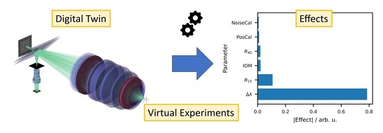
The hardware of the TWI implemented at PTB is based on the MarOpto TWI 60 distributed by Mahr [24]; the setup is similar to a Mach–Zehnder interferometer [12] with some essential differences. A schematic sketch of the TWI is shown in Figure 1. The interferometer is driven by a diode-pumped solid-state laser at a wavelength of λ = 532.3 nm. After a first beam splitter, which divides the illumination light into an optical path for the measurement and a path for reference, the light is expanded and collimated by a lens system and cast onto a microlens array (MLA), which acts as multiple secondary point light sources. The MLA is equipped with a movable shutter array that allows four different arrangements of point light sources to be selected. The light of the point light sources is transformed by the collimator and the objective into variously tilted wavefronts. Depending on the local slope of the SUT, these tilted wavefronts deliver information about different areas of the SUT [13]. The beam stop filters data that would lead to subsampling effects [25]. The current setup of the TWI at PTB allows to measure aspheres with slope deviations of up to 8° from a best-fit sphere (BFS) with a lateral resolution of approx. 30 μm [24]. From five different phase shifted interferograms the setup produces one set of nonoverlapping phase image patches for each shutter position of the MLA [13,15].
To reconstruct the form of the SUT from the obtained data, an inverse problem needs to be solved. The forward model of this inverse problem uses a numerical model for the observed data (the model varies depending on the optical setup of the TWI and the parameterization of the topography of the SUT). The numerical model employed in PTB’s TWI is built using PTB’s in-house simulation software tool, “SimOptDevice” [19]. Among other things, the numerical model implements numerical procedures for ray aiming and ray tracing. The reconstruction of the topography of the SUT is then achieved by adapting the model of the SUT, given by a parametric description of the surface, to obtain the best fit between the simulated and measured data, cf. [15,18,25,26]. For details about how this inverse problem is solved for PTB’s TWI—including preprocessing steps such as data handling, selection of the model parameters, or constraints—we refer to [20].
Accurate knowledge of the optical behavior of the physical instrument is crucial for accurate surface reconstruction. Therefore, a calibration step has to be performed to adjust the numerical model to the real device. For this purpose, a set of known calibration specimens is measured at different measurement positions [14], and the numerical model for the TWI is adjusted based on these measurements. For more details on the calibration step, we again refer to [20].

2.2. Digital Twin

A digital twin of the physical TWI (Figure 2a) has to display the same optical behavior as the real TWI. PTB’s digital twin (Figure 2b) of its TWI is essentially based on the numerical model used for the analysis of the data captured by the TWI (see Section 2.1). To setup this numerical model, the design data of the optical interferometer setup, including the design parameters of the optical components (e.g., geometries of the surfaces, distances, refractive indices) and their arrangement to each other are needed. This allows a detailed simulation of the TWI to be performed. Besides being able to simulate the resulting interferograms, the digital twin can also simulate the effects that deviations from the nominal model of the TWI would have on the measurements, including deviations of the position or tilt of individual optical elements and element groups.
The use of a physical model allows us to gain physical insights into the behavior of the TWI. To estimate the accuracy of the TWI, the parameters of the physical model are chosen differently when simulating data by means of the digital twin as compared to when using the numerical model for solving the inverse problem of SUT topography reconstruction based on the virtual data. Since the size of the disturbances associated with the physical model’s paramters can be elicited from available physical knowledge about the TWI, it is possible to realistically infer the accuracy that can be achieved.
The numerical model of the TWI, however, needs to be very accurate, and a highly accurate calibration of a purely physical model is challenging. We therefore apply a slight phenomenological correction of the physical model. This correction is realized by (small) modifications of optical length and angle in the optical beam path of the simulated rays in two selected planes of the interferometer model. The parameters of these corrections are determined during a calibration (cf. Section 2.1). For details, we refer to [20].

2.3. Simulated Series of Experiments

Virtual experiments were performed using the digital twin of PTB’s TWI. A single virtual experiment consists of a two-step process: the virtual calibration procedure, which is based on a set of virtual calibration samples to calibrate the numerical model of the TWI, followed by the virtual measurement. The virtual measurement uses a virtual specimen to create a set of interference images. These virtual data are then used to reconstruct the topography of the virtual specimen by solving the related inverse problem. The accuracy of the surface reconstruction is assessed by comparing the surface of the virtual specimen with its reconstruction. For this purpose, the root mean square (RMS) error between the reconstructed topography and its (known virtual) ground truth is calculated.

2.4. Virtual Sample Designs

The employed virtual SUT consists of a design topography, i.e., a parameterized asphere, augmented by a randomly generated difference topography parameterized as a set of Zernike coefficients (n = 16, j = 153, [26]). Note that the design topography is known and is utilized for the TWI reconstruction process. Since in a virtual experiment the complete topography of the virtual SUT is known, it is possible to determine the accuracy of its reconstruction from the virtual data.
For the virtual experiments that followed, a strong asphere was utilized as the design topography (Figure 3a). This topography is rotationally symmetric around the vertical axis. A randomly generated difference topography, shown in Figure 3b, is superimposed in the z-direction on the design topography. This topography is not symmetric around the vertical axis and contains a fair amount of irregularities. To take account of effects sensitive to the magnitude of topographic differences, a second difference topography was created by scaling the first in the z-direction by a factor of two. The first and second difference topographies have an RMS, respectively, of 0.27 μm and 0.54 μm.

2.5. Design of Experiment

The TWI is a highly complex device whose measurement accuracy is influenced by a large number of parameters. Each virtual experiment, including the analysis of the virtual data produced, takes a considerable amount of time. With the settings used in this study, one complete virtual experiment (calibration of the model and form measurement) took several hours on a workstation (4 × 16 cores 2.5/3.3 GHz Intel Xeon E7-8867v3 512GB RAM). We therefore pursued the approach of first identifying the main influence parameters that could subsequently be used to explore the TWI’s behavior and the resulting accuracies in more detail.
A common strategy for identifying the main influence parameters in industry and science is the one-factor-at-a-time experimental plan [27]. Here, all parameters except one are fixed to some initial value, and the impact of this one factor is then analyzed based on the results of a (virtual) experiment in which this parameter is set to a different level. Separately examining each parameter in this way does not explore the parameter space in a representative fashion but only within the vicinity of the initial values. While allowing an identification of the impact of each individual parameter, no interactions can be inferred and the accuracy attained in the estimation of the main effects is low, since only two values of the complete data set are taken for the estimation of each main effect. For these reasons, we chose to employ more advanced statistical techniques of experimental design.
Experimental design [21,22,23] applies designs, such as Plackett–Burman [28] designs or fractional factorial designs [21,22,23], to screen key influential parameters that alleviate the aforementioned issues by choosing a subset of a full factorial design. A two-level full factorial design consists of all combinations of the influence parameters at their lower (−) and upper (+) levels. The choice of the (usually small) subset of a full factorial design is made such that balanced and orthogonal plans result. Often, the choice is made to allow the inference not only of the main effects but also of interaction effects up to a specified order. Conference designs [29] provide alternative screening designs that inherit approximately the optimal statistical properties of Plackett–Burman or fractional factorial designs, while additionally enabling a model-independent estimation of main effects.
The advantage of screening designs with N runs such as Plackett–Burman or fractional factorial designs is that main effect estimates have a variance that is O ( 1 / N ) times smaller than the variance of estimates obtained by the one-factor-at-a-time method. Moreover, the parameter space is covered in a much more representative way.
One further aspect of experimental design concerns its control over the complexity of models used for the analysis of the influence parameters. Ideally, this is performed sequentially. In a first step, just a few runs are carried out to identify subgroups of relevant parameters. When using, for example, fractional factorial designs of resolution IV, the effect of interactions between different influence parameters can be taken into account as well. However, due to confounding, the correct subgroup of relevant parameters cannot be deduced exactly. These ambiguities are then resolved by planning corresponding further runs that lead to a higher resolution of the employed design and permit the analysis of a more complex model. This paper shows one example of a controlled sequential strategy that plans new runs to resolve such ambiguities. In this way, reliable results can be achieved at minimum cost. Note that when no interaction is active, the first stage of a low resolution screening design may alone be sufficient.
The parameters involved in the calibration of the TWI are shown along with their − and + levels in Table 1. The parameter IOM represents an “incorrect optical model”. In this study, the IOM is realized as a disturbance of the parameters describing the wavefront manipulators ( C I O M ) that are used for adjusting the optical model of the TWI in the calibration procedure (the source-to-SUT wavefront manipulator RMS error amounted to 0.29 μm and the SUT-to-detector wavefront manipulator RMS error amounted to 67.6 nm). The parameter is used to simulate deviations of the optical model without adding additional elements to the model description. PosCal represents a set of positioning errors ( C P C a l ) of the calibration specimens. To investigate a realistic scenario of positioning errors, one fixed set of positioning errors resulting from a calibration of the measurement device was used. The RMS value of the chosen positioning errors amounted to 3.9 μm. ΔR15 and ΔR40 represent radius deviations of calibration spheres R15 and R40, with R15 being a sphere with a nominal radius of 15 mm and R40 a sphere with a nominal radius of 40 mm. Δλ is the deviation of the laser’s wavelength from its nominal wavelength. In this case, a constant, systematic wavelength deviation was investigated, i.e., the wavelength was stable throughout the experiments but deviated from the wavelength used in the nominal model. NoiseCal is the standard deviation of the Gaussian noise, which is superposed onto the optical path lengths calculated from the interferogram data.
The estimation of main influence parameters within the calibration of the TWI was based on Plackett–Burman screening designs. Plackett–Burman designs are efficient in the sense that main effects can be estimated using a small subset of a full factorial design. For example, a 12 run Plackett–Burman design can be chosen for 11 main effects. For our six parameters in the TWI calibration procedure, the eight runs defined in Table 2 were taken, which at the same time represent a fractional factorial design.
The subsequent simulation of the measurement process of the TWI is less time consuming (approximately 30 min per run for the chosen settings/parameters investigated here), so a more detailed experimental design was utilized. The influence parameters analyzed for the TWI measurement are as follows: the position of the specimen along the x-, y-, and z-axes (Δx, Δy and Δz); the tilt of the specimen along the x-, y-, and z-axes (Δα, Δβ and Δγ); and the standard deviation of the Gaussian noise (NoiseMeas) on the optical path lengths during the measurement (Table 3).
These seven parameters are analyzed using a so-called 2 IV 7 2 fractional factorial design [21]. By systematically reducing the amount of runs of a full factorial design ( 2 7 = 128 ), this two-factor design generates a resolution IV design where main influence parameters are only confounded with higher-order interaction terms of at least three other parameters. This yields a more accurate estimation of the impact of main effects while also allowing interaction effects to be estimated. The required 32 runs for our seven parameters were selected according to [30].

3. Results

3.1. Physical Modifications to the TWI Geometry

To evaluate the capability of the digital twin to simulate physical disturbances of the TWI setup and to demonstrate the impact of the model correction by the wavefront manipulators, the objective lenses component group (see Figure 2b) was shifted along the component’s x-axis (perpendicular to the optical axis) and a virtual experiment was carried out. The RMS error between the virtual specimen topography, and the reconstructed topography from the virtual experiment was used as a measure of the reconstruction quality. Since the virtual experiment included both the calibration and the measurement, two different cases are examined here. In the first case, the objective lenses were shifted prior to the calibration. The second case involved performing the calibration and then shifting the objective lenses before carrying out the measurement. The virtual experiment was performed with two different virtual specimens sharing the same design topography but having differently scaled difference topographies (see Section 2.4). The results are shown in Figure 4. For the shift applied between calibration and measurement, the RMS error shows a linear behavior when plotted against the displacement, while the shift applied before calibration led to an almost constant RMS error (Figure 4). In the latter case, the calibration procedure works to correct the model error and the shift has no effect on the reconstruction result. Where displacement occurs following the calibration, this shift has a direct impact on the accuracy of form reconstruction.

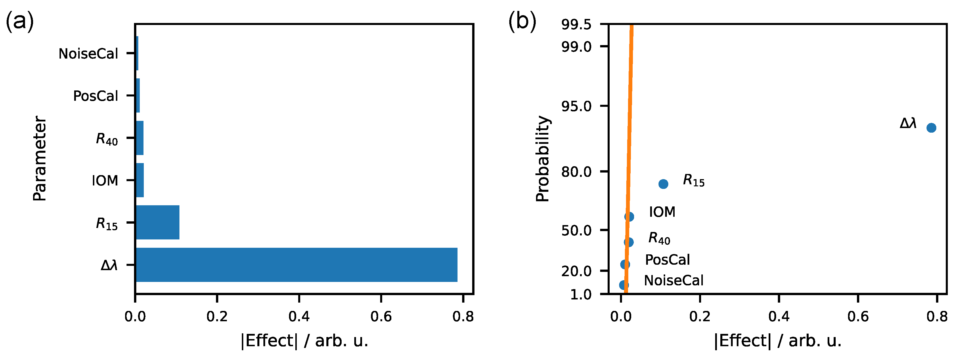
3.2. Identification of Relevant Calibration Parameters

To identify the most relevant parameters, a set of eight virtual experiments was run for various combinations of calibration parameters. The virtual experiments consisted of a calibration of the virtual TWI and a measurement of a virtual SUT using a design topography and a difference topography as specified in Section 2.4. Here, both difference topography scaling factors led to similar results. The accuracy of the virtual experiment was evaluated by means of the RMS error between the virtual SUT and the reconstructed topography, cf. [31].
The screening plan used (cf. Table 2) includes the same amount of runs for the upper (+) and lower (−) levels of each parameter, making the effect of a parameter equal to half of the difference between the average of all RMS values associated with the runs for the upper and lower levels. To approximate a normal distribution of the resulting values, a Box-Cox transformation with parameter θ = 0.086 was applied to the values prior to calculating the effects (cf. [30,32]). The utilized plan does not allow interactions to be estimated, so only the absolutes of the normalized effects of the individual parameters are shown in Figure 5a.
As a result, only the Δλ and the R15 parameters appear to have a greater effect on the reconstruction result of the virtual SUT for the parameters and settings investigated. This is illustrated by a half-normal plot (Figure 5b) where only the main effects related to these two parameters appear to be significant, i.e., their deviation from a straight line cannot be explained as being purely random.

3.3. Sweep over Individual Parameters

Parameter sweeps were performed to further investigate the influence of the Δλ and the R15 parameters. To generate a realistic environment, the non-significant parameters were kept at a fixed level chosen to match their upper levels in the screening design. Since for certain influence parameters spherical errors of the reconstruction result are larger than other form errors, the measurement accuracy was evaluated both with and without the subtraction of a best-fit sphere (BFS) from the reconstruction error. This allows us to distinguish between the spherical error and higher order errors.
In Figure 6, the reconstruction accuracies are depicted for the Δλ parameter ranging from 0 to 0.3 nm. In Figure 6a, the RMS error for two different test topographies is plotted against Δλ both with and without subtraction of the BFS. The difference between the virtual and reconstructed topographies increases linearly. However, for the simulation results obtained with the BFS subtracted from the reconstruction error, the RMS errors are much smaller overall and the rise due to the wavelength deviation is less significant. In Figure 6b, the curvatures of the BFS are shown against Δλ. The relation between the wavelength deviation and the BFS curvature appears to be linear.
The influence of the deviation of the calibration sphere radius ΔR15 is depicted in Figure 7. Similar to the case of Δλ, the subtraction of a BFS from the reconstruction error likewise has a significant influence (approximately factor two) on the RMS error of the topography reconstruction. However, the increase in the RMS error is less prominent here, as seen in Figure 7a, which shows the RMS error in correlation to ΔR15. Nevertheless, the curvature of the best-fit sphere shows a linear relation to the deviation of the calibration sphere radius, as can be seen in Figure 7b.

3.4. Identification of Relevant Measurement Parameters

The analysis of the parameters that influence the calibration was followed by an investigation of the parameters that affect the measurement. For this purpose, a screening plan with 32 individual virtual experiments was generated and applied to two different calibrations. The first was the ideal calibration without disturbances and the second a calibration with disturbances at a level estimated as realistic (cf. Table 1). The experimental design is a fractional factorial design with a resolution of IV and as such allows the analysis of two-factor interactions in addition to the single main effects (cf. Section 2.5).
In Figure 8a, a diagram of the effects of the individual influence parameters is given. Only the NoiseMeas and Δz parameters appear to have a significant influence on the measurement result. Since the resolution of the experimental plan permits a more detailed examination, the two-factor interactions can be calculated as well. This is depicted in the half-normal plot shown in Figure 8b. In addition to the two single-factor effects, the interactions of NoiseMeas * Δz and Δα * Δγ also appear to be significant. But a closer examination of the screening plan reveals that both interactions show the same pattern of positive and negative runs seen in the list of virtual experiments. This means that both effects are confounded and hence indistinguishable at this stage.

3.5. Full Factorial Analysis of Relevant Measurement Parameters

To distinguish between the influence of NoiseMeas * Δz and Δα * Δγ, a full factorial plan of the four parameters Δα, Δγ, NoiseMeas, and Δz was carried out in addition. As the other parameters were observed to be insignificant for the settings investigated here, limiting the investigation to these four parameters therefore seems sufficient. The effects of the full factorial experimental plan are shown in Figure 9a in the form of a bar diagram and in Figure 9b as a half-normal plot.
Apart from the single-factor effects of Δz and NoiseMeas, only the interaction of both has a significant effect. The interaction between Δα and Δγ is not significant. Note further that the Δz effect is much higher than the effect of the noise that was introduced into the simulation.

4. Discussion

The digital twin of the TWI presented in this paper enables the element-wise disturbance of the physical configuration of the measurement system. This allows us to observe the influence of disturbances of single elements within the TWI on the resulting accuracy and makes a systematic study of uncertainty sources possible.
The accuracy of TWI measurements was evaluated using virtual experiments for two different sets of parameters: one associated with the calibration of the virtual TWI and one associated with the virtual measurement. For the settings and parameters investigated during the calibration of the TWI, the influence parameters of laser wavelength deviation (Δλ) and radius deviation of the smaller calibration sphere (R15) were shown to have a significant influence on TWI calibration and the successive measurements. The other parameters investigated here had—at least within the chosen range of their values—no significant effect on the calibration. The subsequent investigations therefore focused primarily on the two significant parameters. A sweep over both influence parameters revealed the degree of correlation between the RMS error and these parameters.
Both the Δλ deviation and the radius deviation of the calibration sphere lead to spherical errors within the reconstructed topography. When the spherical part of the reconstruction error is not taken into account, the remaining error is much smaller. Therefore, particular attention must be given to the origin of spherical errors, which—in addition to being caused by incorrect calibration radii—also arise due to mispositioning of the SUT, especially along the optical axis.
The major influences during TWI measurement are the noise and the deviations of the SUT’s position along the optical axis (Δz). Since the simulation of a TWI measurement is less calculation-intensive than a calibration, and as multiple measurements can be simulated for one calibration, it was possible to perform a higher number of simulated measurements. As a consequence, not only single-factor effects but also two-factor interactions were investigated. However, since the experimental plan has a resolution of IV, two-factor interactions were confounded with each other. This means that the interaction between noise and an SUT positioning error along the optical axis were confounded with the interaction between the tilt along the x-axis and the tilt along the z-axis. To resolve this ambiguity and to gain more information about all interactions, a full factorial design of the four apparently relevant parameters was run. The results revealed that of the two-factor interactions only the interaction between the noise and the positioning error along the optical axis is relevant.

5. Conclusions

In this paper, the digital twin of Physikalisch-Technische Bundesanstalt (PTB)’s tilted-wave interferometer (TWI) was presented as a tool for performing virtual experiments. Virtual experiments allow us to gain insight into resulting accuracies when the physical parameters of the numerical model used in the analysis differ from those used to construct the virtual data. In this way, the most critical parameters of the TWI can be identified. Moreover, the results of the virtual experiment provide a starting point for calculating an uncertainty budget of TWI measurements.
The study presented here identified different parameters that have a high impact on the TWI measurement results. During the calibration procedure of the TWI, the deviation of the wavelength and the radius error of one of the two calibration spheres substantially affected the measurements obtained for the parameters and settings investigated here. In the form reconstruction procedure, the parameters showing the most significant impact were the noise on the optical path lengths and the incorrect positioning of the specimen-under-test (SUT) along the optical axis. We note that these findings are restricted to the set of investigated parameters and the range of their variation, and future studies might reveal further relevant uncertainty sources.
Virtual experiments were shown to provide a useful means for exploring the behavior of a complex optical measurement device. With the aid of a thoroughly designed digital twin, virtual experiments were used to identify those parameters of PTB’s tilted-wave interferometer that have a major influence on the resulting accuracy. Since several potentially relevant parameters were considered and because calculation times for single virtual experiments are high, the statistical technique of experimental design as presented here was applied to guide this process. We conclude that when applied to virtual experiments, experimental design is an efficient approach for tackling complex optical systems involving expensive numerical calculations.

Author Contributions

Conceptualization, G.S., M.M., I.F. and C.E.; methodology, M.M. and G.S.; software, M.S. (Manuel Stavridis); validation, I.F., M.S. (Michael Schulz) and C.E.; formal analysis, M.M.; investigation, G.S.; resources, I.F. and M.S. (Michael Schulz); data curation, M.S. (Manuel Stavridis); writing—original draft preparation, G.S.; writing—review and editing, I.F., M.S. (Michael Schulz) and C.E.; visualization, G.S.; supervision, I.F. and C.E.; project administration, I.F. and C.E. All authors have read and agreed to the published version of the manuscript.

Funding

This research received no external funding.

Institutional Review Board Statement

Not applicable.

Informed Consent Statement

Not applicable.

Data Availability Statement

The data that support the findings of this study are available upon reasonable request from the authors.

Acknowledgments

The authors thank the company Mahr GmbH for providing the Zemax model of the interferometer and for insights into the procedures of the MarOpto TWI 60.

Conflicts of Interest

The authors declare no conflict of interest.

Abbreviations

The following abbreviations are used in this manuscript:
BFSBest-fit sphere
MLAMicrolens array
RMSRoot mean square
SUTSpecimen-under-test
TWITilted-wave interferometer/interferometry

References

  1. Schulz, G. IV Aspheric Surfaces. In Progress in Optics; Wolf, E., Ed.; Elsevier: Amsterdam, The Netherlands, 1988; pp. 349–415. [Google Scholar] [CrossRef]
  2. Hentschel, R.; Braunecker, B.; Tiziani, H.J. (Eds.) Advanced Optics Using Aspherical Elements; SPIE: Bellingham, WA, USA, 2008. [Google Scholar] [CrossRef] [Green Version]
  3. Gutiérrez, C.E. Aspherical lens design. J. Opt. Soc. Am. A 2013, 30, 1719. [Google Scholar] [CrossRef]
  4. Weckenmann, A.; Estler, T.; Peggs, G.; McMurtry, D. Probing Systems in Dimensional Metrology. CIRP Ann. 2004, 53, 657–684. [Google Scholar] [CrossRef]
  5. Van Gestel, N.; Cuypers, S.; Bleys, P.; Kruth, J.P. A performance evaluation test for laser line scanners on CMMs. Opt. Lasers Eng. 2009, 47, 336–342. [Google Scholar] [CrossRef] [Green Version]
  6. Forman, P.F. The Zygo Interferometer System. In Proceedings of the 23rd Annual Technical Symposium, San Diego, CA, USA, WA, USA, 25 December 1979; Hopkins, G.W., Ed.; SPIE: Bellingham, WA, USA, 1979; pp. 41–49. [Google Scholar] [CrossRef]
  7. Poleshchuk, A.G.; Korolkov, V.P.; Nasyrov, R.K.; Asfour, J.M. Computer generated holograms: Fabrication and application for precision optical testing. In Proceedings of the Optical Systems Design, Glasgow, Scotland, UK, 25 September 2008; Duparré, A., Geyl, R., Eds.; SPIE: Bellingham, WA, USA, 2008; p. 710206. [Google Scholar] [CrossRef]
  8. Knauer, M.C.; Kaminski, J.; Hausler, G. Phase measuring deflectometry: A new approach to measure specular free-form surfaces. In Proceedings of the Photonics Europe, Strasbourg, France, 10 September 2004; Osten, W., Takeda, M., Eds.; SPIE: Bellingham, WA, USA, 2004; p. 366. [Google Scholar] [CrossRef]
  9. Petz, M.; Tutsch, R. Reflection grating photogrammetry: A technique for absolute shape measurement of specular free-form surfaces. In Proceedings of the Optics and Photonics 2005, San Diego, CA, USA, 18 August 2005; Stahl, H.P., Ed.; SPIE: Bellingham, WA, USA, 2005; p. 58691. [Google Scholar] [CrossRef]
  10. Kulawiec, A.; Murphy, P.; DeMarco, M. Measurement of high-departure aspheres using subaperture stitching with the Variable Optical Null (VON). In Proceedings of the 5th International Symposium on Advanced Optical Manufacturing and Testing Technologies: Advanced Optical Manufacturing Technologies, Dalian, China, 26–29 April 2010; Yang, L., Namba, Y., Walker, D.D., Li, S., Eds.; SPIE: Bellingham, WA, USA, 2010; p. 765512. [Google Scholar] [CrossRef]
  11. Küchel, M.F. Interferometric measurement of rotationally symmetric aspheric surfaces. Opt. Meas. Syst. Ind. Insp. VI 2009, 7389, 738916. [Google Scholar] [CrossRef]
  12. Greivenkamp, J.E.; Gappinger, R.O. Design of a nonnull interferometer for aspheric wave fronts. Appl. Opt. 2004, 43, 5143. [Google Scholar] [CrossRef] [PubMed]
  13. Garbusi, E.; Pruss, C.; Osten, W. Interferometer for precise and flexible asphere testing. Opt. Lett. 2008, 33, 2973. [Google Scholar] [CrossRef] [PubMed]
  14. Baer, G.; Schindler, J.; Pruss, C.; Siepmann, J.; Osten, W. Calibration of a non-null test interferometer for the measurement of aspheres and free-form surfaces. Opt. Express 2014, 22, 31200. [Google Scholar] [CrossRef]
  15. Pruss, C.; Baer, G.B.; Schindler, J.; Osten, W. Measuring aspheres quickly: Tilted wave interferometry. Opt. Eng. 2017, 56, 111713. [Google Scholar] [CrossRef] [Green Version]
  16. Schindler, J.; Pruss, C.; Osten, W. Simultaneous removal of nonrotationally symmetric errors in tilted wave interferometry. Opt. Eng. 2019, 58, 1. [Google Scholar] [CrossRef]
  17. Harsch, A.; Pruss, C.; Baer, G.; Osten, W. Monte Carlo simulations: A tool to assess complex measurement systems. In Proceedings of the Sixth European Seminar on Precision Optics Manufacturing, Teisnach, Germany, 9–10 April 2019; Schopf, C., Rascher, R., Eds.; SPIE: Bellingham, WA, USA, 2019; p. 24. [Google Scholar] [CrossRef]
  18. Fortmeier, I.; Stavridis, M.; Elster, C.; Schulz, M. Steps towards traceability for an asphere interferometer. In Proceedings of the SPIE Optical Metrology, Munich, Germany, 26 June 2017; Lehmann, P., Osten, W., Albertazzi Gonçalves, A., Eds.; SPIE: Bellingham, WA, USA, 2017; p. 1032939. [Google Scholar] [CrossRef]
  19. Schachtschneider, R.; Stavridis, M.; Fortmeier, I.; Schulz, M.; Elster, C. SimOptDevice: A library for virtual optical experiments. J. Sensors Sens. Syst. 2019, 8, 105–110. [Google Scholar] [CrossRef] [Green Version]
  20. Fortmeier, I.; Stavridis, M.; Schulz, M.; Elster, C. Development of a metrological reference system for the form measurement of aspheres and freeform surfaces based on a tilted-wave interferometer. Meas. Sci. Technol. 2022, 33, 045013. [Google Scholar] [CrossRef]
  21. Box, G.E.P.; Hunter, S.; Hunter, W.G. Statistics for Experimenters: Design, Innovation, and Discovery, 2nd ed.; Wiley-Interscience: Hoboken, NJ, USA, 2005; p. 672. [Google Scholar]
  22. Winer, B.J.; Brown, D.R.; Michels, K.M. Statistical Principles in Experimental Design, 3rd ed.; Mcgraw-Hill Higher Education: New York, NY, USA, 1991; p. 1057. [Google Scholar]
  23. Pukelsheim, F. Optimal Design of Experiments; John Wiley & Sons Inc.: Hoboken, NJ, USA, 1993; p. 384. [Google Scholar]
  24. Mahr GmbH. Mahr TWI 60. Available online: https://metrology.mahr.com/de/produkte/artikel/9061111-tilted-wave-interferometer-maropto-twi-60 (accessed on 13 January 2022).
  25. Schindler, J.; Baer, G.; Pruss, C.; Osten, W. The tilted-wave-interferometer: Freeform surface reconstruction in a non-null setup. In Proceedings of the International Symposium on Optoelectronic Technology and Application 2014, Beijing, China, 3 December 2014; Czarske, J., Zhang, S., Sampson, D., Wang, W., Liao, Y., Eds.; SPIE: Bellingham, WA, USA, 2014; p. 92971. [Google Scholar] [CrossRef]
  26. Fortmeier, I.; Stavridis, M.; Wiegmann, A.; Schulz, M.; Osten, W.; Elster, C. Evaluation of absolute form measurements using a tilted-wave interferometer. Opt. Express 2016, 24, 3393. [Google Scholar] [CrossRef] [PubMed]
  27. Czitrom, V. One-Factor-at-a-Time versus Designed Experiments. Am. Stat. 1999, 53, 126–131. [Google Scholar] [CrossRef]
  28. Plackett, R.L.; Burman, J.P. The Design of Optimum Multifactorial Experiments. Biometrika 1946, 33, 305. [Google Scholar] [CrossRef]
  29. Elster, C.; Neumaier, A. Screening by Conference Designs. Biometrika 1995, 82, 589. [Google Scholar] [CrossRef]
  30. Heckert, N.; Filliben, J.; Croarkin, C.; Hembree, B.; Guthrie, W.; Tobias, P.; Prinz, J. Handbook 151: NIST/SEMATECH e-Handbook of Statistical Methods; NIST Interagency/Internal Report (NISTIR); National Institute of Standards and Technology: Gaithersburg, MD, USA, 2012. [Google Scholar] [CrossRef]
  31. Schachtschneider, R.; Fortmeier, I.; Stavridis, M.; Asfour, J.; Berger, G.; Bergmann, R.B.; Beutler, A.; Blümel, T.; Klawitter, H.; Kubo, K.; et al. Interlaboratory comparison measurements of aspheres. Meas. Sci. Technol. 2018, 29, 055010. [Google Scholar] [CrossRef]
  32. Box, G.E.P.; Cox, D.R. An Analysis of Transformations. J. R. Stat. Soc. Ser. B 1964, 26, 211–243. [Google Scholar] [CrossRef]
Figure 1. Schematic of a tilted-wave interferometer (TWI) consisting of a light source, an object arm, and a reference arm. A laser is used as light source, and its illumination is divided by a beam splitter. Object arm contains a microlens array (MLA), a beam splitter, collimation optics, an objective, specimen under test (SUT), and a beam stop aperture. Light in object arm and reference arm is joined by a beam splitter and cast onto image detector.
Metrology 02 00006 g001
Figure 2. Tilted-wave interferometer (TWI) utilized in this work: (a) physical TWI (MarOpto TWI 60) as found in Physikalisch-Technische Bundesanstalt (PTB) laboratory; (b) digital twin of physical system as simulated by SimOptDevice.
Metrology 02 00006 g002
Figure 3. Topographies used for simulation of TWI process: (a) design topography of a strong asphere; (b) difference topography superimposed on design topography as input for simulation.
Metrology 02 00006 g003
Figure 4. Virtual experiment with objective lenses shifted along x-axis before calibration and between calibration and measurement: RMS error between virtual specimen and reconstructed topography plotted against objective lens displacement.
Metrology 02 00006 g004
Figure 5. Result of design of experiment for calibration parameter: (a) Pareto chart for different calibration parameters; (b) half-normal plot.
Metrology 02 00006 g005
Figure 6. Results of wavelength deviation parameter sweeps: (a) root mean square (RMS) error versus Δλ/nm for different simulated topographies; (b) curvature (r−1) of best-fit sphere (BFS) of reconstruction error in relation to wavelength deviation.
Metrology 02 00006 g006
Figure 7. Results of the R15 calibration sphere radius deviation sweep: (a) RMS error against ΔR15 for different simulated topographies; (b) curvature (r−1) of BFS of reconstruction error in correlation to deviation of ΔR15.
Metrology 02 00006 g007
Figure 8. Results of design of experiment for measurement parameter: (a) Pareto-chart for different measurement parameters; (b) half-normal plot including two-factor interactions.
Metrology 02 00006 g008
Figure 9. Full-factorial experimental design of measurement for parameters Δα, Δγ, NoiseMeas, and Δz: (a) Pareto-chart; (b) half-normal plot.
Metrology 02 00006 g009
Table 1. Influence parameters that were varied during calibration step of virtual experiments.
Parameter+Unit
IOM 0 C I O M -
PosCal 0 C P C a l -
ΔR150400nm
ΔR400400nm
Δλ00.3nm
NoiseCal010nm
Table 2. Plackett–Burman experimental plan for TWI calibration.
12345678
IOM---+-+++
PosCal-+--++-+
ΔR15+-+--+-+
ΔR40--++++--
Δλ++-+-++-
NoiseCal+---+++-
Table 3. Influence parameters that were varied during virtual TWI measurements within virtual experiments.
Parameter+Unit
Δx010μm
Δy010μm
Δz01μm
Δα00.3mrad
Δβ00.3mrad
Δγ00.3mrad
NoiseMeas010nm
Publisher’s Note: MDPI stays neutral with regard to jurisdictional claims in published maps and institutional affiliations.

