Forecast of Omicron Wave Time Evolution

Abstract

The temporal evolution of the omicron wave in different countries is predicted, upon adopting an early doubling time of three days for the rate of new infections with this mutant. The forecast is based on the susceptible–infectious–recovered/removed (SIR) epidemic compartment model with a constant stationary ratio $k=\mu \left(t\right)/a\left(t\right)$ between the infection ($a\left(t\right)$) and recovery ($\mu \left(t\right)$) rates. The assumed fixed early doubling time then uniquely relates the initial infection rate $a_0$ to the ratio k; this way the full temporal evolution of the omicron wave is determined here. Three scenarios (optimistic, pessimistic, intermediate) and the resulting pandemic parameters are considered for 12 different countries. Parameters include the total number of infected persons, the maximum rate of new infections, the peak time and the maximum 7-day incidence per 100,000 persons. The monitored data from Great Britain underwent a clear maximum SDI of 1865 on 7 January 2022. This maximum is a factor 5.0 smaller than our predicted value in the optimistic case and may indicate a dark number of omicron infections of 5.0 in Great Britain. For Germany we predict peak times of the omicron wave ranging from 32 to 38 and 45 days after the start of the omicron wave in the optimistic, intermediate and pessimistic scenario, respectively, with corresponding maximum SDI values of 7090, 13,263 and 28,911. Adopting 1 January 2022 as the starting date our predictions imply the maximum of the omicron wave to be reached between 1 February and 15 February 2022. Rather similar values are predicted for Switzerland. Due to an order of magnitude smaller omicron hospitalization rate, in concert with a high percentage of vaccinated and boosted population, the German health system can cope with a maximum omicron SDI value of 2800 which is about a factor 2.5 smaller than the corresponding value 7090 for the optimistic case. By either reducing the duration of intensive care during peak time, and/or by making use of the nonuniform spread of the omicron wave across Germany, it seems that the German health system can barely cope with the omicron wave and thus avoid triage decisions. The reduced omicron hospitalization rate also causes significantly smaller mortality rates compared to the earlier mutants in Germany. Within the optimistic scenario, we predict 7445 fatalities and a maximum number of 418 deaths/day due to omicron. These numbers range in order of magnitude below the ones known from the beta mutant.

1. Introduction

After being exposed to several COVID-19 outbursts the recently identified omicron mutant threatens many societies worldwide [1,2]. Not many details are known so far about its infection characteristics [3,4] apart from alarming hints (1) that it is spreading at least four times quicker than the $\beta$-mutant with a short doubling time of $t_2=3$ days [5], and (2) that the existing vaccines, tailored to prevent infections from the earlier alpha ($\alpha$), beta ($\beta$), gamma ($\gamma$) and delta ($\delta$) mutants, are less efficient against the action of the omicron mutant especially without the current booster campaigns [5,6,7,8,9]. The $\alpha$, $\beta$, $\gamma$, and $\delta$ mutants have caused the first four COVID-19 waves, respectively [7,8,10,11,12,13,14,15,16,17,18,19,20,21,22,23,24,25], with side effects on societies and markets [26,27,28,29]. Positively, the omicron mutant seems to lead to, on average, milder symptoms and, thus, to smaller hospitalization fractions compared to the earlier mutants [30,31].

With so little detail known today, it is of high interest to quantitatively explore the future time evolution of the omicron mutant under realistic scenarios emanating from the currently taken non-pharmaceutical interventions (NPIs). Of particular interest are reliable estimates of the maximum and total percentage of infected persons caused by the omicron mutant, as they allow for a direct comparison with the available medical capacities in different countries. In the following, we provide these estimates by modeling the time evolution of the omicron wave with the susceptible–infectious–recovered/removed (SIR) epidemic compartment model [32].

As in our earlier analysis [33,34]—hereafter referred to as the KSSIR model—we adopt a constant stationary ratio $k=\mu \left(t\right)/a\left(t\right)=$ const. between the infection ($a\left(t\right)$) and recovery ($\mu \left(t\right)$) rate regulating the transition from susceptible to infected persons and infected to recovered/removed persons in the semi-time case, respectively. The assumed constancy of the ratio k is required to derive the full analytical solution given in Equation (5) below. Despite this restriction the KSSIR model has provided very good agreement of its predictions with the monitored earlier first and second waves [33,34]. As it is so far unclear whether earlier vaccinated persons are unaffected by the omicron mutant, we adopt a worst-case scenario. That is, we treat the vaccinated persons as fully susceptible to the omicron mutant. However, during the calculation of hospitalization and mortality rates we are going to account for the influence of boosted (with vaccines) persons.

The KSSIR model predicted and captured the temporal evolution of the second (beta) wave in several countries convincingly well (Table 1 and Figures 1 and 2 of ref. [33]). The predictions included the maximum rate ${\dot{J}}_{\max }$ of new infections and the total cumulative number ($J_{\infty }$) of infections as well as the initial and final second wave time dependencies and the peak time. For the countries considered in these studies the maximum deviation in the total number of infected persons is at most 13 percent off from the later recorded values. An outstanding property of the KSSIR model is that basically only a single parameter, the ratio k of recovery and infection rates, fully determines the wave evolution in reduced time

$$\tau ={\int }_{t_0}^{t}a\left(\xi \right)d\xi$$

(1)

which can be calculated for any arbitrary but given real time dependence of the infection rate $a\left(t\right)$. The influence of the initial fraction $\eta$ of infected people at the onset of the modeled mutant at time $t_0$ is comparatively minor especially for values of $\eta$ much smaller than unity.

Adopting a constant infection rate $a\left(t\right)=a_0$ is a good approximation for rapidly evolving mutant waves and not only for their initial phases, so that in this case the simple relation $\tau =a_0(t-t_0)$ holds between the reduced and the real time. Moreover, by determining the remaining two decisive parameters k and $a_0$ from the early monitored real time evolution allows us to accurately determine all relevant quantities of the considered outburst. The two parameters k and $a_0$ characterize the specific virus mutant properties, but also vary among different societies depending on their NPIs taken, the quality and ability of their health care systems, and the discipline of the their people in keeping distances, wearing masks and following quarantine measures. As the latter are mainly unchanged during virus mutations, it makes sense to relate the omicron parameters k and $a_0$ to those of the earlier beta mutant. This route will be followed below.

2. Results from the SIR-Model

In terms of the reduced time (1) the KSSIR model equations read

$$\frac{dS}{d\tau }=-SI,\frac{dI}{d\tau }=SI-kI,\frac{dR}{d\tau }=kI$$

(2)

obeying the sum constraint

$$S+I+R=1$$

(3)

at all times. In Equations (2) and (3), S, I and R denote the fractions of susceptible, infected and recovered/removed persons in a population, respectively, subject to the semi-time initial conditions

$$\begin{array}{ccc}\hfill I\left(t_0\right)& =& I(\tau =0)=\eta ,\hfill \\ \hfill S\left(t_0\right)& =& S(\tau =0)=1-\eta ,\hfill \\ \hfill R\left(t_0\right)& =& R(\tau =0)=0.\hfill \end{array}$$

(4)

The rate of new infections and its corresponding cumulative number are given by $j\left(\tau \right)=S\left(\tau \right)I\left(\tau \right)$ and $J\left(\tau \right)={\int }_0^{\tau }d\xi j\left(\xi \right)$, respectively, whereas $\dot{J}\left(t\right)=a\left(t\right)j\left(\tau \right)$ and $J\left(t\right)=J\left(\tau \right)$.

2.1. Exact Results

In terms of J the exact solution of the KSSIR model in the semi-time case is given by [34]

$$\tau ={\int }_{\eta }^J\frac{dy}{n\left(y\right)},n\left(y\right)=(1-y)[y+kϵ+kln(1-y)]$$

(5)

with $ϵ=-ln(1-\eta )$. The remaining SIR quantities are given by $J\left(\tau \right)$ as $S\left(\tau \right)=1-J\left(\tau \right)$, $I\left(\tau \right)=J\left(\tau \right)+kϵ+kln[1-J(\tau \left)\right]$ and $R\left(\tau \right)=-k[ϵ+ln(1-J\left(\tau \right)\left)\right]$. Differentiating Equation (5) with respect to $\tau$ readily yields for the rate of new cases

$$j\left(\tau \right)=\frac{dJ}{d\tau }=(1-J)[J+kϵ+kln(1-J)]$$

(6)

As shown before [34], one obtains the final cumulative fraction $J_{\infty }$ of infected persons without the explicit inversion of the solution (5) to $J\left(\tau \right)$,

$$J_{\infty }=\underset{\tau \to \infty }{lim}J\left(\tau \right)=1+k{W}_0\left(\alpha \right),$$

(7)

with $\alpha =-(1-\eta )k^{-1}{e}^{-1/k}$. The maximum rate of new infections

$$j_{\max }=(1-J_0)(1-J_0-k)=\frac{k^2}{4}({[1+W_{-1}\left({\alpha }_0\right)]}^2-1),$$

(8)

occurs at

$$J_0=1+\frac{k}{2}{W}_{-1}\left({\alpha }_0\right),{\alpha }_0=\frac{2\alpha }{e}$$

(9)

in terms of the principal ($W_0$) and non-principal ($W_{-1}$) solution of Lambert’s Equation [35], the well-known and documented Lambert functions. We emphasize that for small values of $\eta \ll 1$ the results (7) and (9) are basically independent of the value of $\eta$ and determined by the ratio k. The first Equation (8) implies

$$J_0\left(k\right)=1-\frac{k}{2}-\sqrt{{\left(\frac{k}{2}\right)}^2+j_{\max }}$$

(10)

2.2. Approximate Results

Very accurate approximations have been obtained [35] for

$$\begin{array}{ccc}\hfill j_{\max }\left(k\right)& \simeq & \frac{{(1-k)}^2(7+8k)}{14(2-k)(1+k)},\hfill \\ \hfill J_{\infty }\left(k\right)& \simeq & \frac{7+k-8k^2}{7},\hfill \end{array}$$

(11)

so that Equation (10) provides the approximation

$$J_0\left(k\right)\simeq 1-\frac{k}{2}-\sqrt{{\left(\frac{k}{2}\right)}^2+\frac{{(1-k)}^2(7+8k)}{14(2-k)(1+k)}}.$$

(12)

Note that for small $k<1/8$ the exact expressions (7), (9), and (10) are still useful as the approximation gives values slightly larger than unity for $J_{\infty }$.

The occurrence of the maximum rate of new infections (8) at positive values of the reduced peak time ${\tau }_{\max }>0$ requires values of $k<1-2\eta$. In this case [34] the reduced peak time is well approximated by

$${\tau }_{\max }\simeq \frac{1}{c_3}\mathrm{artanh}\frac{2c_3}{c_1+\frac{2c_0}{J_0-\eta }},$$

(13)

with $c_0=\eta (1-\eta )$ and $c_1=1-k-2\eta$,

$$\begin{array}{ccc}\hfill c_2& =& \frac{j_{\max }-c_0-c_1(J_0-\eta )}{{(J_0-\eta )}^2},\hfill \\ \hfill c_3& =& \sqrt{{\left(\frac{c_1}{2}\right)}^2-c_0{c}_2},\hfill \end{array}$$

(14)

while the reduced time dependence of the rate of new infections is well approximated as

$$\frac{j\left(\tau \right)}{j_{\max }}=\left\{\begin{array}{cc}\hfill {\left(\frac{sinh\left(c_3{\tau }_m\right)}{sinh\left(c_3\tau \right)+\sqrt{\frac{j_{\max }}{c_0}}sinh\left[c_3({\tau }_m-\tau )\right]}\right)}^2& \hfill \mathrm{for}\tau \le {\tau }_m\\ \frac{e^{d_1(\tau -{\tau }_m)}}{{\left(1+\frac{j_{\max }}{d_1(J_{\infty }-J_0)}\left[e^{d_1(\tau -{\tau }_m)}-1\right]\right)}^2}\hfill & \hfill \mathrm{for}\tau \ge {\tau }_m\end{array}\right.$$

(15)

with $d_1=J_{\infty }-(1-k)$. For a stationary infection rate $a_0$ the corresponding real peak time is given by

$$t_{\mathrm{peak}}=t_0+\frac{{\tau }_{\max }}{a_0}.$$

(16)

Likewise, the early asymptotic reduced time behavior is well approximated [35] by

$$j_{\mathrm{early}}(\tau \ll {\tau }_{\max )})\simeq A{e}^{(1-k)\tau },$$

(17)

corresponding to the early asymptotic real time behavior

$${\dot{J}}_{\mathrm{early}}\left(t\right)=a\left(t\right)j_{\mathrm{early}}\left(\tau \left(t\right)\right).$$

(18)

In the considered case of a stationary infection rate Equation (18) reduces to

$${\dot{J}}_{\mathrm{early}}\left(t\right)=a_{0}j(\tau =a_0(t-t_0))=A{a}_0{e}^{(1-k)a_0(t-t_0)},$$

(19)

implying for the early doubling time defined by ${\dot{J}}_{\mathrm{early}}(t+t_2)=2{\dot{J}}_{\mathrm{early}}\left(t\right)$ that

$$t_2=\frac{ln2}{a_0(1-k)}=\frac{ln2}{a_0-{\mu }_0},$$

(20)

where we inserted $k={\mu }_0/a_0$ in the case of stationary infection and recovery rates. Equation (20) will be used in the following two sections in two different ways.

The maximum 7-day incidence value per ${10}^5$ persons is calculated by integrating

$$\mathrm{SDI}={10}^5{\int }_{t_{\max }-3.5}^{t_{\max }+3.5}dt\dot{J}\left(t\right),$$

(21)

it is only slightly smaller than the estimate $\mathrm{SDI}\simeq$$7\times {10}^5{\dot{J}}_{\max }$ from the maximum rate. At late times after the maximum half-decay time is given by

$$t_{1/2}\simeq \frac{ln2}{a_0{d}_1}=\frac{0.693}{a_0[J_{\infty }-(1-k)]}$$

(22)

3. Consequences of Early 3-Day Doubling Time

For the omicron mutant the early doubling time of $t_{2,\mathrm{omicron}}=3$ days has been reported [3,4] in South Africa, Great Britain and Denmark. Adopting this value for all countries considered then provides according to Equation (20) for the omicron mutant the relation

$$a_0^{\mathrm{omicron}}=\frac{ln2}{3(1-k_{\mathrm{omicron}})}=\frac{0.231}{1-k_{\mathrm{omicron}}}{\mathrm{days}}^{-1}$$

(23)

throughout. Using this relation in all results of the last section to eliminate $a_0$ we find that all quantities of interest are solely determined by the parameter $k_{\mathrm{omicron}}$. Particularly for the peak time (16) we obtain

$$t_{\mathrm{peak},\mathrm{omicron}}=t_0+4.328{\tau }_{\max }(1-k_{\mathrm{omicron}}),$$

(24)

whereas the maximum rate of new infections can be expressed as

$$\begin{array}{ccc}\hfill {\dot{J}}_{\max ,\mathrm{omicron}}\left(k_{\mathrm{omicron}}\right)& =& a_0^{\mathrm{omicron}}{j}_{\max }\left(k_{\mathrm{omicron}}\right)=\frac{0.231j_{\max }\left(k_{\mathrm{omicron}}\right)}{1-k_{\mathrm{omicron}}}\hfill \\ & \simeq & \frac{0.0165(1-k_{\mathrm{omicron}})(7+8k_{\mathrm{omicron}})}{(2-k_{\mathrm{omicron}})(1+k_{\mathrm{omicron}})}.\hfill \end{array}$$

(25)

Likewise the real time dependence of the rate of new infections with Equation (14) is given by

$${\dot{J}}_{\mathrm{omicron}}\left(t\right)=\frac{0.231j\left(\frac{0.231(t-t_0)}{1-k_{\mathrm{omicron}}}\right)}{1-k_{\mathrm{omicron}}}$$

(26)

In Figure 1, we display the resulting dependence of $J_{\infty }$, $t_{\max }-t_0={\tau }_{\max }/a_0^{\mathrm{omicron}}$ and ${\dot{J}}_{\max }=a_0^{\mathrm{omicron}}{j}_{\max }$ as functions of the parameter $k_{\mathrm{omicron}}\in [0,1]$.

It can be seen that $J_{\infty }$ and ${\dot{J}}_{\max }$ decrease with increasing values of $k_{\mathrm{omicron}}$, and that this effect if unaffected by the initial fraction $\eta$ of infected persons, except at very large values of $k_{\mathrm{omicron}}$ close to unity. Obviously, for comparatively small values of the total number of infected persons $J_{\infty }$ and the maximum rate of newly infected persons ${\dot{J}}_{\max }$ large values of the ratio $k_{\mathrm{omicron}}$ are required. Alternatively, the reduced time of maximum ${\tau }_{\max }$ decreases with increasing values of $k_{\mathrm{omicron}}$ as long as $k_{\mathrm{omicron}}$ is much smaller than $1-2\eta$.

4. Omicron Forecast in Individual Countries

Next we calculate the second wave doubling time $t_2^{\beta }$ for the countries listed in

Table 1. Second wave parameters $a_0^{\beta }$ in days${}^{-1}$, $k_{\beta }$, initial fraction ${\eta }_{\beta }$, and the inferred second doubling time $t_2^{\beta }$ in days. For the omicron mutant in all countries we adopt $t_2^{\mathrm{omicron}}$ to calculate the ratio of the the two doubling times $r=t_2^{\beta }/t_2^{\mathrm{omicron}}$.

Country	${\mathit{a}}_0^{\mathit{\beta }}$	${\mathit{k}}_{\mathit{\beta }}$	${\mathit{\eta }}_{\mathit{\beta }}$	${\mathit{t}}_2^{\mathit{\beta }}$	${\mathit{t}}_2^{\mathbf{omicron}}$	$\mathit{r}={\mathit{t}}_2^{\mathit{\beta }}/{\mathit{t}}_2^{\mathbf{omicron}}$
ITA	0.13	0.823	$1.1\times {10}^{-4}$	30.1	3.0	10.03
AUT	0.43	0.898	$1.8\times {10}^{-5}$	15.8	3.0	5.27
DNK	2.48	0.972	$3.6\times {10}^{-5}$	10.0	3.0	3.33
DEU	0.45	0.907	$1.1\times {10}^{-5}$	16.6	3.0	5.53
CHE	0.44	0.892	$2.2\times {10}^{-5}$	14.6	3.0	4.87
GBR	0.44	0.874	$4.6\times {10}^{-5}$	12.5	3.0	4.17
FRA	0.17	0.868	$1.0\times {10}^{-4}$	30.9	3.0	10.30
BEL	0.53	0.893	$1.8\times {10}^{-4}$	12.2	3.0	4.07
NLD	0.37	0.926	$3.4\times {10}^{-5}$	25.3	3.0	8.43
RUS	0.03	0.801	$6.9\times {10}^{-3}$	116.1	3.0	38.70
SWE	0.58	0.919	$8.0\times {10}^{-9}$	14.8	3.0	4.93
USA	0.22	0.868	$9.5\times {10}^{-4}$	23.9	3.0	7.97

, upon making use of the earlier inferred parameter values [33] $a_0^{\beta }$ and $k_{\beta }$ for the second wave, i.e., caused by the $\beta$-mutant. Adopting the short omicron doubling time $t_2^{\mathrm{omicron}}=3$ days for all countries, we obtain the ratio r of the doubling times (last column of Table 1).

With Equation (20) we infer for this ratio

$$r=t_2^{\beta }/t_2^{\mathrm{omicron}}=\frac{a_0^{\mathrm{omicron}}(1-k_{\mathrm{omicron}})}{a_0^{\beta }(1-k_{\beta })},$$

(27)

readily yielding the relation

$$a_0^{\mathrm{omicron}}(1-k_{\mathrm{omicron}})=r{a}_0^{\beta }(1-k_{\beta }).$$

(28)

For each country we consider 3 possible omicron scenarios:

(1)

the optimistic case with $k_{\mathrm{omicron}}=k_{\beta }$ so that the increase in the ratio r is solely due to the increase in the stationary infection rate

$$a_0^{\mathrm{omicron}}=r{a}_0^{\beta }$$

(29)

As noted earlier the larger the value of $k_{\mathrm{omicron}}$ the smaller the total cumulative number of infections $J_{\infty }$ and the maximum rate of new infections $j_{\max }$ will be. This justifies the classification of this case as optimistic.

(2)

the pessimistic scenario with $a_0^{\mathrm{omicron},\mathrm{pess}}=a_0^{\beta }$ so that the increase in the ratio r is solely due to the decrease in the ratio k

$$k_{\mathrm{omicron},\mathrm{pess}}=1-r(1-k_{\beta })$$

(30)

Clearly, with these small values of $k_{\mathrm{omicron}}$ the resulting total cumulative number of infections $J_{\infty }$ and the maximum rate of new infections $j_{\max }$ will be highest, justifying the classification of this case as pessimistic. In four countries (ITA, FRA, RUS, USA) the resulting $k_{\mathrm{omicron},\mathrm{pess}}$ is negative which cannot be. In these cases we use $k_{\mathrm{omicron},\mathrm{pess}}=0$ and $a_0^{\mathrm{omicron},\mathrm{pess}}=0.231$.

(3)

the intermediate case with

$$a_0^{\mathrm{omicron},\mathrm{inter}}=\frac{r}{2}{a}_0^{\beta },$$

(31)

where half of the increase in the ratio r stems from the increase in the stationary infection rate. Then as a consequence

$$k_{\mathrm{omicron},\mathrm{inter}}=2k_{\beta }-1$$

(32)

In

Table 2. Forecast of the omicron mutant for the optimistic case, i.e., $a_0=a_0^{\mathrm{omicron},\mathrm{optim}}$, $k=k_{\mathrm{omicron},\mathrm{optim}}$, and initial fraction $\eta ={\eta }_{\beta }$ from Table 1 for this table. Columns list the final cumulative fraction $J_{\infty }$ of infected persons, the maximum (dimensionless) rate $j_{\max }$ of new infections, the cumulative fraction $J_0$ of infected persons at peak time, the reduced peak time ${\tau }_{\max }$, the peak time $t_{\max }-t_0$ in days, and the SDI, the maximum 7-day incidence per ${10}^5$ persons. Country names are abbreviated by their ${\alpha }_3$ codes.

Optimistic Scenario
${\mathit{\alpha }}_{\mathbf{3}}$	${\mathit{a}}_{\mathbf{0}}$	$\mathit{k}$	${\mathit{J}}_{\mathbf{\infty }}$	${\mathit{j}}_{\mathbf{max}}$	${\dot{\mathit{J}}}_{\mathbf{max}}$	${\mathit{J}}_{\mathbf{0}}$	${\mathit{\tau }}_{\mathbf{max}}$	${\mathit{t}}_{\mathbf{max}}-{\mathit{t}}_{\mathbf{0}}$	SDI
ITA	1.304	0.823	0.33	0.0139	0.018	0.160	35.6	27days	12,725
AUT	2.265	0.898	0.20	0.0049	0.011	0.097	68.9	30days	7716
DNK	8.267	0.972	0.06	0.0004	0.004	0.028	130.1	16days	2424
DEU	2.490	0.907	0.18	0.0041	0.010	0.089	79.0	32days	7090
CHE	2.141	0.892	0.21	0.0054	0.012	0.102	64.0	30days	8148
GBR	1.833	0.874	0.24	0.0073	0.013	0.118	51.3	28days	9392
FRA	1.751	0.868	0.25	0.0080	0.014	0.123	43.5	25days	9853
BEL	2.155	0.893	0.21	0.0055	0.012	0.101	44.3	21days	8250
NLD	3.120	0.926	0.14	0.0026	0.008	0.071	77.4	25days	5751
RUS	1.161	0.801	0.39	0.0219	0.025	0.173	10.7	9days	17,773
SWE	2.861	0.919	0.16	0.0031	0.009	0.078	175.6	61days	6216
USA	1.753	0.868	0.26	0.0087	0.015	0.122	26.0	15days	10,650

,

Table 3. Forecast of the omicron mutant for the pessimistic case, i.e., $a_0=a_0^{\mathrm{omicron},\mathrm{pess}}$ and $k=k_{\mathrm{omicron},\mathrm{pess}}$.

Pessimistic Scenario
${\mathit{\alpha }}_{\mathbf{3}}$	${\mathit{a}}_{\mathbf{0}}$	$\mathit{k}$	${\mathit{J}}_{\mathsf{\infty }}$	${\mathit{j}}_{\mathbf{max}}$	${\dot{\mathit{J}}}_{\mathbf{max}}$	${\mathit{J}}_{\mathbf{0}}$	${\mathit{\tau }}_{\mathbf{max}}$	${\mathit{t}}_{\mathbf{max}}-{\mathit{t}}_{\mathbf{0}}$	SDI
ITA	0.231	0.000	1.000	0.2500	0.058	0.500	9.2	40days	40,414
AUT	0.430	0.463	0.836	0.0984	0.042	0.379	18.8	44days	29,621
DNK	2.480	0.907	0.181	0.0041	0.010	0.089	65.6	27days	7148
DEU	0.450	0.485	0.812	0.0918	0.041	0.369	20.4	45days	28,911
CHE	0.440	0.474	0.824	0.0950	0.042	0.374	18.7	42days	29,259
GBR	0.440	0.475	0.823	0.0949	0.042	0.374	17.3	39days	29,208
FRA	0.231	0.000	1.000	0.2500	0.058	0.500	9.2	40days	40,414
BEL	0.530	0.565	0.721	0.0696	0.037	0.331	17.0	32days	25,819
NLD	0.370	0.376	0.911	0.1249	0.046	0.412	15.5	42days	32,336
RUS	0.231	0.000	1.000	0.2500	0.058	0.500	5.0	22days	40,422
SWE	0.580	0.600	0.675	0.0602	0.035	0.312	43.1	74days	24,408
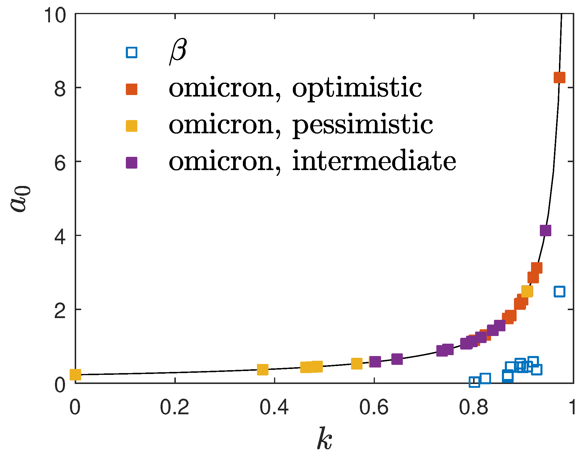
USA	0.231	0.000	1.000	0.2500	0.058	0.500	7.0	30days	40,419

and

Table 4. Forecast of the omicron mutant for the intermediate case, i.e., $a_0=a_0^{\mathrm{omicron},\mathrm{inter}}$ and $k=k_{\mathrm{omicron},\mathrm{inter}}$.

Intermediate Scenario
${\mathit{\alpha }}_{\mathbf{3}}$	${\mathit{a}}_{\mathbf{0}}$	$\mathit{k}$	${\mathit{J}}_{\mathsf{\infty }}$	${\mathit{j}}_{\mathbf{max}}$	${\dot{\mathit{J}}}_{\mathbf{max}}$	${\mathit{J}}_{\mathbf{0}}$	${\mathit{\tau }}_{\mathbf{max}}$	${\mathit{t}}_{\mathbf{max}}-{\mathit{t}}_{\mathbf{0}}$	SDI
ITA	0.652	0.646	0.613	0.0489	0.032	0.286	21.4	33days	22,307
AUT	1.132	0.796	0.378	0.0181	0.021	0.182	41.0	36days	14,328
DNK	4.133	0.944	0.110	0.0015	0.006	0.054	90.9	22days	4462
DEU	1.245	0.814	0.347	0.0152	0.019	0.168	46.7	38days	13,263
CHE	1.071	0.784	0.398	0.0201	0.022	0.191	38.2	36days	15,060
GBR	0.917	0.748	0.458	0.0267	0.024	0.218	31.0	34days	17,109
FRA	0.876	0.736	0.477	0.0290	0.025	0.226	26.8	31days	17,797
BEL	1.078	0.786	0.396	0.0199	0.021	0.189	28.6	27days	14,979
NLD	1.560	0.852	0.281	0.0099	0.016	0.137	48.0	31days	10,832
RUS	0.580	0.602	0.678	0.0627	0.036	0.307	8.8	15days	25,466
SWE	1.431	0.838	0.305	0.0117	0.017	0.148	96.2	67days	11,748
USA	0.876	0.736	0.479	0.0295	0.026	0.226	18.3	21days	18,110

we calculate the forecast for the omicron mutant for these three scenarios, respectively. Figure 2 visualizes the relationship between $a_0$ and k and the location of the three regimes for the 12 countries, and Figure 3 shows the time dependence of $\dot{J}\left(t\right)$ and cumulative fraction $J\left(t\right)$ of infected persons for all 12 countries.

It is obvious from these three tables that in European countries, apart from Russia with limited data reliability, Denmark has the shortest peak time of the omicron wave ranging from 16 to 22 and 27 days after the start of the omicron wave in the optimistic, intermediate and pessimistic scenario, respectively. The corresponding predicted maximum 7-day incidence values per ${10}^5$ persons (SDI) are 2424, 4462 and 7148, respectively. At the date of original submission (10 January 2022) of this manuscript the well-monitored data of Denmark [36] indicated that the SDI saturated at a value of 2478 which would be in excellent agreement with our predicted value in the optimistic case. However, today (28 January 2022) it is clear that this earlier apparent saturation has been an intermediate plateau because the Danish SDI values started increasing again up to a maximum value of 5327 today. Therefore it is clear that the monitored Danish data are reproduced better by our intermediate or pessimistic scenario. On the other hand the monitored data from Great Britain underwent a clear maximum SDI of 1865 on 7 January 2022. This maximum is a factor 5.0 smaller than our predicted value in the optimistic case. This great factor may be regarded as an estimate of the dark number of omicron infections in Great Britain.

Among the considered countries sofar as of today besides Great Britain also USA and Italy now have declining SDI values. In the remaining nine countries the monitored SDI values are still increasing.

Regarding Germany we predict peak times of the omicron wave ranging from 32 to 38 and 45 days after the start of the omicron wave in the optimistic, intermediate and pessimistic scenario, respectively, with corresponding maximum SDI values of 7090, 13,263 and 28,911, respectively. Adopting 1 January 2022 as the starting date our predictions imply that the maximum of the omicron wave is reached between 1 February and 15 February 2022. In the optimistic case the total cumulative number of omicron infections will be 0.180 but can go up high to 0.812 in the pessimistic case. The late half decay times are 3.2 to 3.5 and 5.2 days in the optimistic, intermediate and pessimistic case, respectively.

Rather similar values are predicted for Switzerland. Here the peak times of the omicron wave range from 30 to 36 and 42 days after the start and the corresponding maximum SDI values are 8148, 15,060 and 29,259. Employing the same starting date, the maximum of the omicron wave is reached between 31 January and 13 February 2022. In the optimistic case the total cumulative number of omicron infections will be 0.208 but can go up high to 0.824 in the pessimistic case. The late half decay times are 3.2 to 3.6 and 5.3 days in the optimistic, intermediate and pessimistic cases.

5. Medical Consequences for Germany

5.1. Tolerable Maximum 7-Day Incidence Value

We have argued earlier [36] that the German health system can cope with maximum SDI values of $280/\left(hm\right)$ without any triage decisions, where m in months denotes the average duration of intensive care with access to breathing apparatus for seriously infected persons, and h in units of percent indicates the percentage of people seriously infected needing access to breathing instruments in hospitals. For the earlier $\alpha$ and $\beta$ mutants the value of $h=1$ turned out reasonable. Fortunately, for the omicron variant a substantial 70–90 percent reduction of hospitalization has been reported from studies in South Africa [37] and Great Britain [38], as compared to earlier mutants. This strong reduction is predominantly caused by the high percentage of persons with boosted vaccination.

We therefore adopt here the value of $h_{\mathrm{omicron}}=0.1$, i.e., only one out of 1000 new infections with the omicron mutant needs to be hospitalised. Consequently, the German health system can cope with maximum omicron SDI value of $2800/m$ which is about a factor 2.5 smaller than the maximum omicron SDI value 7090 in the optimistic case. By either (1) reducing the duration of intensive care during this period of maximum to $m=0.5$, and/or (2) by making use of the nonuniform spread of the omicron wave across Germany, appearing first in the northern states and considerably later in the southern and eastern states, combined with mutual help in hospital capacities, it seems that the German health system can cope with the omicron wave avoiding triage decisions.

5.2. Fatality Rates and Total Number of Fatalities

As before [33,36] we assume that every second hospitalised person eventually dies from the omicron virus so that the omicron mortality rate is $f_{\mathrm{omicron}}=0.5h_{\mathrm{omicron}}=5\times {10}^{-4}$ which is one order of magnitude smaller than the mortality rates of the earlier mutants. Consequently, the total fatality rate is given by $D_{\infty }=f_{\mathrm{omicron}}{J}_{\infty }N$, where $N=82.7$ million denotes the German population. Likewise the maximum death rate is $d_{\max }=f_{\mathrm{omicron}}N{\dot{J}}_{\max }$. In the optimistic scenario one obtains $D_{\infty }=7445$ and $d_{\max }=418$ per day which are about one order of magnitude smaller than the beta fatality rate and total number of fatalities of the second wave [33]. The main reason for these comparatively small numbers is the order of magnitude smaller hospitalization rate of the omicron mutant compared to the earlier more deadly mutants.

However, in the less likely pessimistic scenario the fatality numbers increase by a factor 4.5 to to $D_{\infty }$ = 33,576 and $d_{\max }=1708$ which are about half of the fatality values of the second wave.

6. Summary and Conclusions

Adopting an early doubling time of three days for the rate of new infections with the omicron mutant the temporal evolution of the omicron wave in different countries is predicted. The predictions are based on the susceptible-infectious-recovered/removed (SIR) epidemic compartment model with a constant stationary ratio $k=\mu \left(t\right)/a\left(t\right)$ between the infection ($a\left(t\right)$) and recovery ($\mu \left(t\right)$) rate. The fixed early doubling time then uniquely relates the initial infection rate $a_0$ to the ratio k, which therefore determines the full temporal evolution of the omicron waves.

As all considered countries have been exposed to earlier waves of the COVID-19 virus, we relate the parameters $a_0$ and k to those of the well-studied second wave. In the optimistic case, we assumed that the decrease in the early doubling time of the omicron mutant as compared to the beta mutant is solely due to a corresponding increase in the initial infection rate $a_0$ whereas the ratio k is the same as for the beta mutant. In the pessimistic case, we assumed that the decrease in the early doubling times is fully caused by a corresponding decrease in the ratio k, whereas the initial infection rate is the same as for the beta mutant. In the intermediate scenario, half of the decrease in the early doubling time was assigned to a corresponding increase in the initial infection rate and a corresponding decrease in the ratio k. For 12 countries, these three scenarios (optimistic, pessimistic and intermediate) were considered and the resulting pandemic parameters were calculated. These include the total number of infected persons, the maximum rate of new infections, the peak time and the maximum 7-day incidence per 100,000 persons.

Among the considered European countries, Denmark has the smallest omicron peak time. Around 11 January 2022, the SDI values exhibited an intermediate plateau, but since then the SDI values have increased again to values more than 5000; therefore, the Danish data may be better explained by the intermediate or pessimistic scenario. In Great Britain, the monitored SDI values exhibited a clear maximum of 1865 on 7 January 2022, indicating a high number of omicron infections of about 5.0 in this country. For Germany, we predict peak times of the omicron wave ranging from 32 to 38 and 45 days after the start of the omicron wave in the optimistic, intermediate and pessimistic scenario, respectively, with corresponding maximum SDI values of 7090, 13,263 and 28,911, respectively. Adopting 1 January 2022 as the starting date our predictions implies that the maximum of the omicron wave is reached between 1 February and 15 February 2022. In the optimistic case, the total cumulative number of omicron infections will be 0.180, but can rise to 0.812 in the pessimistic case. The latter half, decay times are 3.2 to 3.5 and 5.2 days in the optimistic, intermediate and pessimistic case, respectively.

Rather similar values are predicted for Switzerland. Here, the peak times of the omicron wave range from 30 to 36 and 42 days after the start and the corresponding maximum SDI values are 8148, 15,060 and 29,259, respectively. Here, with the same starting date, the maximum of the omicron wave is reached between 31 January and 13 February 2022. Here, in the optimistic case, the total cumulative number of omicron infections will be 0.208, but can rise to 0.824 in the pessimistic case. The latter half decay times are 3.2 to 3.6 and 5.3 days in the optimistic, intermediate and pessimistic case, respectively.

Adopting an order of magnitude, the lower omicron hospitalization rate is thanks to the high percentage of vaccinated and boosted population, we conclude that the German health system can cope with maximum omicron SDI value of 2800, which is about a factor 2.5 smaller than the maximum omicron SDI value 7090 in the optimistic case. By either reducing the duration of intensive care during this period of maximum, and/or by making use of the nonuniform spread of the omicron wave across Germany, it seems that the German health system can barely cope with the omicron wave while avoiding triage decisions.

The reduced omicron hospitalization rate also causes significantly smaller mortality rates compared to the earlier mutants in Germany. In the optimistic scenario, one obtains for the total number of fatalities $D_{\infty }=7445$ and for the maximum death rate $d_{\max }=418$ per day, which are about one order of magnitude smaller than the beta fatality rate and total number. In the less likely pessimistic scenario, these numbers increase by a factor 4.5.

Note added in proof (23 February 2022): The monitored data for Germany and Switzerland displayed that the SDI values have reached their maximum values 1594.2 and 2913.8 on 10 February 2022 and 1 February 2022, respectively [39]. These values are in excellent agreement with the predictions in the optimistic case made here, and indicate dark numbers of omicron infections of 4.4 and 2.8, respectively, in these two countries.

References

- Kupferschmidt, K.; Vogel, G. COVID-19 How bad is Omicron? Some clues are emerging. Science 2021, 374, 1304–1305. [Google Scholar] [CrossRef] [PubMed]
- Skipper, M. The global response to Omicron is making things worse. Nature 2021, 600, 190. [Google Scholar]
- Viana, R.; Moyo, S.; Amoako, D.G.; Tegally, H.; Scheepers, C.; Althaus, C.L.; Anyaneji, U.J.; Bester, P.A.; Boni, M.F.; Ch, M.; et al. Rapid epidemic expansion of the SARS-CoV-2 Omicron variant in southern Africa. Nature 2022, 13, 469. [Google Scholar] [CrossRef] [PubMed]
- Barnard, R.C.; Davies, N.G.; Pearson, C.A.B.; Jit, M.; Edmunds, W.J. Projected epidemiological consequences of the Omicron SARS-CoV-2 variant in England, December 2021 to April 2022. medRxiv 2021. [Google Scholar] [CrossRef]
- Torjesen, I. Covid restrictions tighten as omicron cases double every two to three days. BMJ-Br. Med. J. 2021, 375, n3051. [Google Scholar] [CrossRef]
- COVID; CDC; Response Team. SARS-CoV-2 B.1.1.529 (Omicron) Variant—United States, December 1–8, 2021. MMWR-Morb. Mortal. Wkly. Rep. 2021, 70, 1731–1734. [Google Scholar] [CrossRef]
- Karim, S.S.A.; Karim, Q.A. Omicron SARS-CoV-2 variant: A new chapter in the COVID-19 pandemic. Lancet 2021, 398, 2126. [Google Scholar] [CrossRef]
- Mahase, E. COVID-19: Do vaccines work against omicron-and other questions answered. BMJ-Br. Med. J. 2021, 375, n3062. [Google Scholar] [CrossRef]
- Kannan, S.R.; Spratt, A.N.; Sharma, K.; Chand, H.S.; Byrareddy, S.N.; Singh, K. Omicron SARS-CoV-2 variant: Unique features and their impact on pre-existing antibodies. J. Autoimmun. 2022, 126, 102779. [Google Scholar] [CrossRef]
- Kutscher, E. Preparing for Omicron as a covid veteran. BMJ-Br. Med. J. 2021, 375, n3021. [Google Scholar] [CrossRef]
- Fuss, F.K.; Weizman, Y.; Tan, A.M. COVID-19 Pandemic: How effective are preventive control measures and is a complete lockdown justified? A comparison of countries and states. Covid 2022, 2, 18–46. [Google Scholar] [CrossRef]
- Torjesen, I. COVID-19: Omicron may be more transmissible than other variants and partly resistant to existing vaccines, scientists fear. BMJ Brit. Med. J. 2021, 375, n2943. [Google Scholar] [CrossRef]
- Khataniar, A.; Pathak, U.; Rajkhowa, S.; Jha, A.N. A comprehensive review of drug repurposing strategies against known drug targets of COVID-19. Covid 2022, 2, 148–167. [Google Scholar] [CrossRef]
- Banerjee, I.; Robinson, J.; Banerjee, I.; Sathian, B. Omicron: The pandemic propagator and lockdown instigator—What can be learnt from South Africa and such discoveries in future. Nepal J. Epidemiol. 2021, 11, 1126–1129. [Google Scholar] [CrossRef] [PubMed]
- Kannan, S.; Ali, P.S.S.; Sheeza, A. Omicron (B.1.1.529)—Variant of concern—Molecular profile and epidemiology: A mini review. Eur. Rev. Med. Pharm. Sci. 2021, 25, 8019–8022. [Google Scholar]
- Fang, F.; Shi, P.Y. Omicron: A drug developer’s perspective comment. Emerg. Microbes Infect. 2022, 11, 208–211. [Google Scholar] [CrossRef]
- Wang, Y.; Zhang, L.; Li, Q.; Liang, Z.; Li, T.; Liu, S.; Cui, Q.; Nie, J.; Wu, Q.; Qu, X.; et al. The significant immune escape of pseudotyped SARS-CoV-2 variant Omicron. Emerg. Microbes Infect. 2022, 11, 1–5. [Google Scholar]
- Bonanni, P.; Cantón, R.; Gill, D.; Halfon, P.; Liebert, U.G.; Crespo, K.A.N.; Martín, J.J.P.; Trombetta, C.M. The role of serology testing to strengthen vaccination initiatives and policies for COVID-19 in Europe. Covid 2021, 1, 20–38. [Google Scholar] [CrossRef]
- Dhawan, M.; Priyanka, O.P.C. Omicron SARS-CoV-2 variant: Reasons of emergence and lessons learnt. Int. J. Surg. 2022, 97, 106198. [Google Scholar] [CrossRef]
- Choudhary, O.P.; Dhawan, M.; Priyanka. Omicron variant (B.1.1.529) of SARS-CoV-2: Threat assessment and plan of action. Int. J. Surg. 2022, 97, 106187. [Google Scholar] [CrossRef]
- Oshinubi, K.; Amakor, A.; Peter, O.J.; Rachdi, M.; Demongeot, J. Approach to COVID-19 time series data using deep learning and spectral analysis methods. AIMS Bioeng. 2022, 9, 1–21. [Google Scholar] [CrossRef]
- Duradoni, M.; Fiorenza, M.; Guazzini, A. When Italians follow the rules against COVID infection: A psychological profile for compliance. Covid 2021, 1, 246–262. [Google Scholar] [CrossRef]
- Bettuzzi, S.; Gabba, L.; Cataldo, S. Efficacy of a polyphenolic, standardized green tea extract for the treatment of COVID-19 syndrome: A proof-of-principle study. Covid 2021, 1, 2–12. [Google Scholar] [CrossRef]
- Ganasegeran, K.; Ch’ng, A.S.H.; Looi, I. What is the estimated COVID-19 reproduction number and the proportion of the population that needs to be immunized to achieve herd immunity in Malaysia? A mathematical epidemiology synthesis. Covid 2021, 1, 13–19. [Google Scholar] [CrossRef]
- Mahase, E. COVID-19: Omicron and the need for boosters. BMJ-Br. Med. J. 2021, 375, n3079. [Google Scholar] [CrossRef] [PubMed]
- Kou, G.; Xiao, H.; Cao, M.; Lee, L.H. Optimal computing budget allocation for the vector evaluated genetic algorithm in multi-objective stochastic optimization. Automatica 2021, 129, 109599. [Google Scholar] [CrossRef]
- Xiao, H.; Xiong, X.; Chen, W. Introduction to the special issue on Impact of COVID-19 and cryptocurrencies on the global financial market. Financ. Innov. 2021, 7, 27. [Google Scholar] [CrossRef]
- Neslihanoglu, S. Linearity extensions of the market model: A case of the top 10 cryptocurrency prices during the pre-COVID-19 and COVID-19 periods. Financ. Innov. 2021, 7, 38. [Google Scholar] [CrossRef]
- Zhang, F.; Narayan, P.K.; Devpura, N. Has COVID-19 changed the stock return-oil price predictability pattern? Financ. Innov. 2021, 7, 61. [Google Scholar] [CrossRef]
- Christie, B. COVID-19: Early studies give hope omicron is milder than other variants. BMJ-Br. Med. J. 2021, 375, n3144. [Google Scholar] [CrossRef]
- Dyer, O. COVID-19: Omicron is causing more infections but fewer hospital admissions than delta, South African data show. BMJ-Br. Med. J. 2021, 375, n3104. [Google Scholar] [CrossRef] [PubMed]
- Estrada, E. COVID-19 and SARS-CoV-2. Modeling the present, looking at the future. Phys. Rep. 2020, 869, 1–51. [Google Scholar] [CrossRef] [PubMed]
- Kröger, M.; Schlickeiser, R. Verification of the accuracy of the SIR model in forecasting based on the improved SIR model with a constant ratio of recovery to infection rate by comparing with monitored second wave data. R. Soc. Open Sci. 2021, 8, 211379. [Google Scholar] [CrossRef] [PubMed]
- Schlickeiser, R.; Kröger, M. Analytical solution of the SIR-model for the temporal evolution of epidemics: Part B. Semi-time case. J. Phys. A 2021, 54, 175601. [Google Scholar] [CrossRef]
- Kröger, M.; Schlickeiser, R. Analytical solution of the SIR-model for the temporal evolution of epidemics. Part A: Time-independent reproduction factor. J. Phys. A 2020, 53, 505601. [Google Scholar] [CrossRef]
- Schlickeiser, R.; Kröger, M. Reasonable limiting of 7-day incidence per hundred thousand and herd immunization in Germany and other countries. Covid 2021, 1, 130–136. [Google Scholar] [CrossRef]
- Wolter, N.; Jassat, W.; Walaza, S. Early assessment of the clinical severity of the SARS-CoV-2 Omicron variant in South Africa: A data linkage study. Lancet 2022, 399, 437. [Google Scholar] [CrossRef]
- Sheikh, A.; Kerr, S.; Woolhouse, M.; McMenamin, J.; Robertson, C. Severity of Omicron Variant of Concern and Vaccine Effectiveness against Symptomatic Disease: National Cohort with Nested Test Negative Design Study in Scotland; The University of Edinburgh Preprint Server: Edinburgh, Scotland, 2021; Available online: https://www.research.ed.ac.uk/en/publications (accessed on 22 December 2021).
- Siekmann, M. Corona-in-Zahlen; Fuchsstr. 1, 50823 Cologne, Germany. 2022. Available online: https://www.corona-in-zahlen.de/weltweit/ (accessed on 22 February 2022).
Figure 1.
(a) , (b) , and (c) as a function of the only parameter for different values of the initial fraction of infected persons in the case of an early 3-day doubling time.
Figure 2.
Location of the considered values of and k for the omicron mutant in the investigated 12 countries with the adopted 3-day early doubling times. The symbols represent the values for the earlier beta mutant. The solid black line is Equation (23).
Figure 3.
Time dependence of the daily rate of newly infected persons, , as well as the cumulative fraction of infected persons, , for all 12 countries.