Helmholtz–Galerkin Regularizing Technique for the Analysis of the THz-Range Surface-Plasmon-Mode Resonances of a Graphene Microdisk Stack

Abstract

The aim of this paper is the accurate and efficient analysis of the surface-plasmon-mode resonances of a graphene microdisk stack in the terahertz range. By means of suitable generalized boundary conditions and Fourier series expansion, the problem is formulated in terms of sets of one-dimensional integral equations in the vector Hankel transform domain for the harmonics of the surface current densities. In virtue of the Helmholtz decomposition, the unknowns are replaced by the corresponding surface curl-free and divergence-free contributions. An approximate solution is achieved by means of the Galerkin method. The proper selection of expansion functions reconstructing the physical behavior of the surface current densities leads to a fast-converging Fredholm second-kind matrix equation, whose elements are accurately and efficiently evaluated by means of a suitable analytical procedure in the complex plane. It is shown that the surface-plasmon-mode resonance frequencies upshift by increasing the number of disks and by decreasing the distance between the disks, and that new resonances can arise for small with respect to the radius distances between the disks, resembling the dipole-mode resonances of the dielectric disk, while, for larger distances, the surface-plasmon-mode resonances can split.

1. Introduction

Thin objects have been receiving the attention of the electromagnetic scientific community because of the different areas of application ranging from antennas and frequency-selecting surfaces to tree leaves modeling, just to cite some notable examples. A recent impetus to the research in that field has been given by the discovery of new materials showing amazing mechanical, thermal, optical, and electronic properties. Among them, the most popular is undoubtedly graphene, which is a planar monolayer of carbon atoms organized in a honeycomb lattice [1,2,3]. It works similar to a zero band-gap semiconductor, whose conductivity can be tuned with the aid of a DC bias, which translates into a graphene chemical potential. The ability to support the propagation of surface plasmon polaritons in the terahertz (THz) and infrared ranges with moderate losses, strong wave localization, and tunability opens new scenarios unimaginable for the noble metals, for which such a phenomenon occurs at higher frequencies [4]. As a result, on the finite-size graphene structures, the reflection of the surface plasmon polaritons at the edges creates surface-plasmon-mode resonances (SPRs) with moderate Q-factors at the THz and infrared frequencies, which can be tuned by changing the graphene chemical potential. This interesting phenomenon is currently studied and has already found applications in the design of novel biosensors [5,6,7] and antennas [8].

As the graphene can be interpreted as a truly 2D material, the formulation of an electromagnetic problem involving patterned graphene structures can be conveniently carried out by means of uniquely solvable surface-singular integral equations for the surface current density, providing that the boundary, radiation, and power boundedness conditions are fulfilled. Despite their ostensible simplicity, the numerical solution of such kinds of equations can be burdensome, leading to ill-conditioned and/or dense matrix equations. Moreover, the convergence of the discretization scheme adopted is questionable because no theorems are available to generally state the existence of a solution and, in any case, the convergence of an approximate solution to the exact one cannot be guaranteed.

In general, only the equations of the Fredholm second kind are not affected by those problems [9]. For them, the existence of the solution and the convergence of a discretization scheme preserving the Fredholm second-kind nature of the integral equation is guaranteed. Unfortunately, the integral formulations of electromagnetic problems involving objects with wedges or open surfaces lead to singular integral equations at which Fredholm’s theory cannot be applied. On the other hand, such equations can be converted to Fredholm second-kind equations by means of the methods of analytical regularization [10,11]. The reasoning is, in principle, very simple: extract and analytically invert a suitable part of the integral operator including the most singular one. The operator to be analytically inverted can be the static part, the high-frequency part, a canonical-shape part, etc. of the integral operator, depending on the problem at hand, and it can be inverted by means of functional techniques such as the Wiener–Hopf, Cauchy, Titchmarsh, Abel, Riemann–Hilbert Problem, and the separation of variables.

Another way to overcome the problems detailed above consists in individuating a suitable discretization scheme so that the resulting matrix equation is of the Fredholm second kind. This is tantamount to saying that the analytical regularization and the discretization are carried out in a single step. The desired result can be achieved by individuating an orthonormal set of eigenfunctions of a suitable singular part of the integral operator, including the most singular one, and assuming such a set as an expansion basis of the unknown in a Galerkin scheme. In this way, the Galerkin projection, which acts as a perfect preconditioner, leads to the diagonalization of the considered singular part of the integral operator and to the compactness in $l^2$ of the remaining part. Therefore, if the free term has a bounded $l^2$-norm, the obtained matrix equation is of the Fredholm second kind in $l^2$. Such an approach, called the method of analytical preconditioning [10,11], has been extensively used to study electromagnetic propagation, radiation, and scattering problems [12,13,14,15,16,17,18,19,20].

The analysis of the scattering by thin planar disks has been receiving the attention of the scientific community for decades [21,22,23,24,25,26,27,28]. The reasons are to be found in the possibility of drastically simplifying the formulation of the problem. Indeed, the zero-thickness or the very small thickness with respect to the wavelength, and the azimuthal symmetry allow the formulation of the problem in terms of infinite sets of one-dimensional integral equations in the vector Hankel transform (VHT) domain obtained by means of suitable generalized boundary conditions and Fourier series expansion. A recently developed technique to solve such equations has been proposed in [29,30,31,32,33,34,35,36] for the analysis of the scattering from perfectly electrically conducting, resistive, including graphene, and dielectric disks. It is based on the combination of the Helmholtz decomposition, which leads to scalar unknowns in the VHT domain, and the method of analytical preconditioning. The selection of expansion functions reconstructing the physical behavior of the unknowns guarantees the fast convergence of the discretization scheme. Moreover, the coefficient matrix elements, expressed as one-dimensional improper integrals of oscillating functions, are evaluated by means of analytical techniques in the complex plane that drastically speed up the computation time.

In this paper, the above convergent method is adopted to study the effect of the coupling in a graphene microdisk stack on the SPRs in the THz range. The generalization of the procedure developed in [33] allows the accurate and efficient evaluation of the mutual coupling integrals independently of the distance between the disks. Due to the disks’ coupling, the SPR frequencies upshift by increasing the number of the disks and by decreasing the distance between the disks. Moreover, new resonances can arise for small with respect to the radius distances between the disks, resembling the dipole-mode resonances of the dielectric disk, while, for larger distances, the SPRs can split.

This paper is organized as follows. Section 2 is devoted to the formulation of the problem. In Section 3, the analytical regularization method adopted is briefly explained. The numerical evaluation of the coefficient matrix is discussed in Section 4. The numerical results are presented in Section 5, and the conclusions summarized in Section 6.

2. Formulation

The geometry of the problem is depicted in Figure 1: a plane wave impinges onto a graphene microdisk stack in free space consisting of L identical and equiaxial monolayer graphene disks of radius a of the order of micrometers, located at the abscissas $z=z_i$ for $i=1,2,\dots L$ in a cylindrical coordinate system, $\left(\rho ,\varphi ,z\right)$, with the z axis orthogonal to the disks’ surfaces, while the plane wave incidence angles are denoted by ${\theta }_0$ and ${\varphi }_0$.

Each disk can be seen as a truly 2D planar object, which can be modeled as a resistive surface. In turn, the surface resistivity level is given by the reciprocal of the surface conductivity of the graphene. Because the disks’ radius is larger than 50 nm, the edge effects on the graphene surface conductivity, appearing for structures smaller than 100 nm, can be neglected. Hence, the model for the surface conductivity devised for an infinite graphene sheet can be used [37]. Moreover, without a magnetostatic bias field, the graphene material can be assumed isotropic [38], which results in a scalar surface conductivity, ${\sigma }_s$. According to the Kubo formalism [38], ${\sigma }_s$ can be generally written as the superposition of an intraband contribution and an interband contribution. As the interband contribution can be neglected at all frequencies below the visible range, ${\sigma }_s$ is dominated by the intraband contribution in the THz and infrared ranges. Hence, in our analysis, which is focused on the THz range, the following expression is assumed for the surface conductivity:

$${\sigma }_s=-\mathrm{j}\frac{e^2{k}_{B}T}{\pi {\hslash }^2\left(\omega -\frac{\mathrm{j}}{t_{relax}}\right)}\left(\frac{{\mu }_c}{k_{B}T}+2\mathit{ln}\left(e^{-\frac{{\mu }_c}{k_{B}T}}+1\right)\right),$$

(1)

where $\omega =2\pi f$ is the angular frequency, f is the frequency, e is the electron charge, $k_B$ is the Boltzmann constant, T is the temperature, $\hslash$ is the reduced Planck constant, $t_{relax}$ is the relaxation time of an electron, and ${\mu }_c$ is the chemical potential.

The electromagnetic scattering problem at hand can be formulated as a boundary value problem for the Maxwell equations by imposing the following resistive boundary conditions on the disks’ surfaces [39]:

$$\widehat{z}\times \left(\underset{\_}{E}\left(\rho ,\varphi ,z_i^{+}\right)+\underset{\_}{E}\left(\rho ,\varphi ,z_i^{-}\right)\right)\times \widehat{z}=2R_i{\underset{\_}{J}}_i\left(\rho ,\varphi \right)$$

(2)

for $\rho \le a$, $0\le \varphi <2\pi$, and $i=1,2,\dots L$, where $\underset{\_}{E}\left(·\right)$ denotes the total electric field, the surface current density ${\underset{\_}{J}}_i\left(\rho ,\varphi \right)=J_{i,\rho }\left(\rho ,\varphi \right)\widehat{\rho }+J_{i,\varphi }\left(\rho ,\varphi \right)\widehat{\varphi }=\widehat{z}\times \left(\underset{\_}{H}\left(\rho ,\varphi ,z_i^{+}\right)-\underset{\_}{H}\left(\rho ,\varphi ,z_i^{-}\right)\right)$ is the jump across the i-th disk’s surface of the total magnetic field $\underset{\_}{H}\left(·\right)$, and $R_i=1/{\sigma }_{s,i}$ and ${\sigma }_{s,i}$ are, respectively, the surface resistivity and conductivity of the i-th disk. Moreover, the uniqueness of the solution is guaranteed providing the Silver–Muller radiation condition and the power boundedness condition [10,40].

By means of the well-known approach based on the second Green’s formula, the problem can be equivalently formulated in terms of a system of L integral equations on the disks’ surfaces involving the surface current densities, the Green’s function, and their normal to the disks derivatives [40]. The proper choice of the Green’s function allows the radiation condition to be automatically satisfied. Moreover, the power boundedness condition binds the behavior of the surface current densities at the disks’ rims and then defines the functional space to which the currents belong. Under these conditions, the obtained system of surface integral equations is uniquely solvable.

The problem can be deeply simplified exploiting its azimuthal symmetry. As a matter of fact, all the involved functions can be expanded in Fourier series. Hence, taking advantage of the orthogonality of the azimuthal harmonics, each surface integral equation can be equivalently rewritten as an infinite set of one-dimensional integral equations for the azimuthal harmonics of the surface current densities. By invoking the VHT of order n (VHT_n) [21],

$${\widetilde{\underset{\_}{\mathit{J}}}}^{\left(n\right)}\left(w\right)=\underset{0}{\overset{+\infty }{{\displaystyle \int }}}{\underset{\_}{\underset{\_}{\mathit{H}}}}^{\left(n\right)}\left(w\rho \right){\underset{\_}{\mathit{J}}}^{\left(n\right)}\left(\rho \right)\rho d\rho ,$$

(3)

where

$${\underset{\_}{\underset{\_}{\mathit{H}}}}^{\left(n\right)}\left(w\rho \right)=\left(\begin{array}{cc}{J}_n^{\text{′}}\left(w\rho \right)& \frac{n{J}_n\left(w\rho \right)}{\left(w\rho \right)}\\ \frac{n{J}_n\left(w\rho \right)}{\left(w\rho \right)}& J_n^{\text{′}}\left(w\rho \right)\end{array}\right)$$

(4)

is the kernel, $J_{\nu }(\cdot )$ and $J_{\nu }^{\text{′}}(\cdot )$ are, respectively, the Bessel function of the first kind and order $\nu$ and its first derivative with respect to the argument [41], and the symbols

$${\underset{\_}{\mathit{J}}}^{\left(n\right)}\left(\rho \right)=\left(\begin{array}{c}{J}_{\rho }^{\left(n\right)}\left(\rho \right)\\ -\mathrm{j}{J}_{\varphi }^{\left(n\right)}\left(\rho \right)\end{array}\right)$$

(5)

$${\widetilde{\underset{\_}{\mathit{J}}}}^{\left(n\right)}\left(w\right)=\left(\begin{array}{c}{\tilde{J}}_{\mathrm{C}}^{\left(n\right)}\left(w\right)\\ -\mathrm{j}{\tilde{J}}_{\mathrm{D}}^{\left(n\right)}\left(w\right)\end{array}\right)$$

(6)

have been introduced, and assuming $\sqrt{k_0^2-w^2}=-\mathrm{j}\sqrt{-k_0^2+w^2}$, the components of the n-th harmonic of the total electric field can be written as

$${\underset{\_}{\mathit{E}}}^{\left(n\right)}\left(\rho ,z\right)={\underset{\_}{\mathit{E}}}^{\mathrm{inc}\left(n\right)}\left(\rho ,z\right)+{\displaystyle \sum }_{j=1}^L\underset{0}{\overset{+\infty }{{\displaystyle \int }}}{\underset{\_}{\underset{\_}{\mathit{H}}}}^{\left(n\right)}\left(w\rho \right)\underset{\_}{\underset{\_}{\tilde{\mathit{G}}}}\left(w\right){\underset{\_}{\tilde{\mathit{J}}}}_j^{\left(n\right)}\left(w\right)e^{-\mathrm{j}\left|z-z_j\right|\sqrt{k_0^2-w^2}}wdw,$$

(7)

$$E_z^{\left(n\right)}\left(\rho ,z\right)=E_z^{\mathrm{inc}\left(n\right)}\left(\rho ,z\right)-\mathrm{j}\frac{\mathrm{sgn}\left(z\right)}{2\omega {\epsilon }_0}{\displaystyle \sum }_{j=1}^L\underset{0}{\overset{+\infty }{{\displaystyle \int }}}{J}_n\left(w\rho \right){\underset{\_}{\tilde{J}}}_{j,\mathrm{C}}^{\left(n\right)}\left(w\right)e^{-\mathrm{j}\left|z-z_j\right|\sqrt{k_0^2-w^2}}{w}^{2}dw,$$

(8)

where

$$\underset{\_}{\underset{\_}{\tilde{\mathit{G}}}}\left(w\right)=\left(\begin{array}{cc}{G}_{\mathrm{C}}\left(w\right)& 0\\ 0& G_{\mathrm{D}}\left(w\right)\end{array}\right)=\left(\begin{array}{cc}-\frac{\sqrt{k_0^2-w^2}}{2\omega {\epsilon }_0}& 0\\ 0& -\frac{\omega {\mu }_0}{2\sqrt{k_0^2-w^2}}\end{array}\right)$$

(9)

is the spectral domain Green’s function, $\mathrm{sgn}\left(·\right)$ denotes the signum function [41], ${\epsilon }_0$, ${\mu }_0$, and $k_0=\omega \sqrt{{\epsilon }_0{\mu }_0}$ are, respectively, the free-space dielectric permittivity, magnetic permeability, and wavenumber, ${\underset{\_}{\tilde{\mathit{J}}}}_i^{\left(n\right)}\left(w\right)$ is the VHT_n of the n-th harmonic of the surface current density on the i-th disk, ${\underset{\_}{\mathit{J}}}_i^{\left(n\right)}\left(\rho \right)$, while ${\underset{\_}{\mathit{E}}}^{\mathit{inc}\left(n\right)}\left(·\right)$ and $E_z^{\mathrm{inc}\left(n\right)}\left(·\right)$ are the components of the n-th harmonic of the incident electric field. Hence, starting from Equation (2) and Formula (7), the following system of spectral domain singular integral equations can be readily stated:

$${\displaystyle \sum }_{j=1}^L\underset{0}{\overset{+\infty }{{\displaystyle \int }}}{\underset{\_}{\underset{\_}{\mathit{H}}}}^{\left(n\right)}\left(w\rho \right)\left(\underset{\_}{\underset{\_}{\tilde{\mathit{G}}}}\left(w\right)-{\delta }_{i,j}{R}_i\underset{\_}{\underset{\_}{\mathit{I}}}\right){\underset{\_}{\tilde{\mathit{J}}}}_j^{\left(n\right)}\left(w\right)e^{-\mathrm{j}\left|z_i-z_j\right|\sqrt{k_0^2-w^2}}wdw=-{\underset{\_}{\mathit{E}}}^{\mathrm{inc}\left(n\right)}\left(\rho ,z_i\right)$$

(10)

for $\rho \le a$, $n\in \mathbb{Z}$, and $i=1,2,\dots L$, where ${\delta }_{i,j}$ is the Kronecker delta function and $\underset{\_}{\underset{\_}{\mathit{I}}}$ is the identity operator.

By virtue of the Helmholtz decomposition [42], the n-th harmonic of the i-th surface current density can be represented as the superposition of a surface curl-free contribution, ${\underset{\_}{\mathit{J}}}_{i,\mathrm{C}}^{\left(n\right)}\left(\rho \right)$, and a surface divergence-free contribution, ${\underset{\_}{\mathit{J}}}_{i,\mathrm{D}}^{\left(n\right)}\left(\rho \right)$. It has been shown in [32] that the VHT_n of such contributions has only one nonvanishing component, i.e.,

$${\underset{\_}{\tilde{\mathit{J}}}}_{i,\mathrm{C}}^{\left(n\right)}\left(w\right)=\left(\begin{array}{c}{\tilde{J}}_{i,\mathrm{C}}^{\left(n\right)}\left(w\right)\\ 0\end{array}\right),$$

(11)

$${\underset{\_}{\tilde{\mathit{J}}}}_{i,\mathrm{D}}^{\left(n\right)}\left(w\right)=\left(\begin{array}{c}0\\ -\mathrm{j}{\tilde{J}}_{i,\mathrm{D}}^{\left(n\right)}\left(w\right)\end{array}\right),$$

(12)

hence, they can be suitably chosen as new unknowns in the spatial domain, bringing the advantage of being able to handle scalar unknowns into the spectral domain.

3. Analytical Regularization

No closed-form solution is available for the system of integral Equation (10); hence, a discretization scheme has to be adopted, whose convergence deserves to be discussed. Indeed, due to the singular nature of the obtained integral equations, the existence of a solution cannot be stated. Moreover, even if a solution exists, no theorem asserts the convergence of a general discretization scheme to the solution itself as the truncation order tends to infinity. However, by expanding the unknowns in eigenfunctions of the most singular part of the integral operators and adopting the Galerkin scheme, Galerkin projection acts as a perfect preconditioner and the system of integral equations is recast as a matrix equation of the Fredholm second kind. As a result, the existence of the solution and the convergence of the discretization scheme can be claimed.

Therefore, the proper selection of the expansion functions is a key point. Suitable expansions of the unknowns have been introduced in [33]. They are Neumann series of weighted Bessel functions [43], which constitute complete sets of orthonormal eigenfunctions of the most singular part of the involved integral operators:

$${\tilde{J}}_{i,T}^{\left(n\right)}\left(w\right)={\displaystyle \sum }_{h=-1+{\delta }_{n,0}}^{+\infty }{\gamma }_{i,T,h}^{\left(n\right)}{\tilde{f}}_{T,h}^{\left(n\right)}\left(w\right)$$

(13)

for $n\in \mathbb{Z}$ and $i=1,2,\dots L$, where

$${\tilde{f}}_{T,h}^{\left(n\right)}\left(w\right)={\beta }_{T,h}^{\left(n\right)}\frac{J_{\left|n\right|+2h+p_T+1}\left(aw\right)}{w^{p_T}},$$

(14)

$T=\mathrm{C},\mathrm{D}$; ${\delta }_{n,m}$ is the Kronecker delta; ${\gamma }_{i,T,h}^{\left(n\right)}$, with ${\gamma }_{i,\mathrm{D},-1}^{\left(n\right)}=\frac{\mathrm{j}\mathrm{sgn}\left(n\right)\left|n\right|! }{\mathsf{\Gamma }\left(\left|n\right|+3/2\right)}\sqrt{\frac{a\left(\left|n\right|+1/2\right)}{2\left|n\right|}}{\gamma }_{i,\mathrm{C},-1}^{\left(n\right)}$ for $n\ne 0$, denotes the general expansion coefficient; ${\beta }_{T,h}^{\left(n\right)}=\sqrt{2\left(\left|n\right|+2h+p_T+1\right)}$; $p_{\mathrm{C}}=3/2$; $p_{\mathrm{D}}=1$; and $\mathsf{\Gamma }\left(·\right)$ is the Gamma function [41]. With such a choice, the vanishing of the currents for $\rho >a$ is guaranteed at each truncation order. Moreover, the behavior of the n-th harmonic of the surface current densities around the disks’ centers is factorized and the field’s behavior at the disks’ rims [44] is reconstructed, thus ensuring that a few expansion functions are enough to achieve accurate results.

According to the procedure detailed in [29,33], by expanding the unknowns as in (13) and projecting Equation (10) on the i-th disk onto the basis functions of the unknowns on the same disk, the following matrix equation is obtained for the n-th harmonic of the unknowns:

$${\mathit{X}}_i^{\left(n\right)}+{\displaystyle \sum }_{j=1}^L{\mathit{A}}_{i,j}^{\left(n\right)}{\mathit{X}}_j^{\left(n\right)}={\mathit{B}}_i^{\left(n\right)}$$

(15)

for $i=1,2,\dots L$, where ${\mathit{X}}_i^{\left(n\right)}$ is the vector of the expansion coefficients of the n-th harmonic of the unknowns on the i-th disk, the general element of the matrix operator ${\mathit{A}}_{i,j}^{\left(n\right)}$ is proportional to

$$I_{T,i,j,h,k}^{\left(n\right)}=\underset{0}{\overset{+\infty }{{\displaystyle \int }}}{G}_T\left(w\right){\tilde{f}}_{T,h}^{\left(n\right)}\left(w\right){\tilde{f}}_{T,k}^{\left(n\right)}\left(w\right)e^{-\mathrm{j}\left|z_i-z_j\right|\sqrt{k_0^2-w^2}}wdw,$$

(16)

and ${\mathit{B}}_i^{\left(n\right)}$, which is the n-th harmonic of the free-term vector related to the i-th disk, is defined in [34]. Following the line of reasoning proposed in [29,33], it is possible to demonstrate that the matrix operator ${\mathit{A}}^{\left(n\right)}={\left\{{\mathit{A}}_{i,j}^{\left(n\right)}\right\}}_{i,j=1}^L$ is a compact operator in $l^2$ and the free term ${\mathit{B}}^{\left(n\right)}={\left\{{\mathit{B}}_i^{\left(n\right)}\right\}}_{i=1}^L$ has a bounded $l^2$-norm. Hence, Equation (15) is a Fredholm second-kind matrix operator equation in $l^2$.

4. Numerical Evaluation of the Coefficient Matrix

By means of the recurrence formula for the Bessel functions [41], it is simple to rewrite the integrals in (16) as follows:

$$I_{\mathrm{C},i,j,h,k}^{\left(n\right)}=\frac{{\beta }_{\mathrm{C},k}^{\left(n\right)}{\beta }_{\mathrm{C},h}^{\left(n\right)}}{2\omega {\epsilon }_0}{\overline{I}}_{i,j,k+\frac{5}{4},h+\frac{5}{4}}^{\left(n\right)}-\frac{\omega {\mu }_0{a}^2}{4{\beta }_{\mathrm{C},k}^{\left(n\right)}{\beta }_{\mathrm{C},h}^{\left(n\right)}}\left({\overline{I}}_{i,j,k+\frac{3}{4},h+\frac{3}{4}}^{\left(n\right)}+{\overline{I}}_{i,j,k+\frac{7}{4},h+\frac{3}{4}}^{\left(n\right)}+{\overline{I}}_{i,j,k+\frac{3}{4},h+\frac{7}{4}}^{\left(n\right)}+{\overline{I}}_{i,j,k+\frac{7}{4},h+\frac{7}{4}}^{\left(n\right)}\right),$$

(17)

$$I_{\mathrm{D},i,j,h,k}^{\left(n\right)}=-\frac{\omega {\mu }_{0}a}{2}\frac{{\beta }_{\mathrm{D},h}^{\left(n\right)}}{{\beta }_{\mathrm{D},k}^{\left(n\right)}}\left({\overline{I}}_{i,j,k+\frac{1}{2},h+1}^{\left(n\right)}+{\overline{I}}_{i,j,k+\frac{3}{2},h+1}^{\left(n\right)}\right),$$

(18)

where

$${\overline{I}}_{i,j,\nu ,\eta }^{\left(n\right)}=\underset{0}{\overset{+\infty }{{\displaystyle \int }}}\frac{e^{-\mathrm{j}\left|z_i-z_j\right|\sqrt{k_0^2-w^2}}}{\sqrt{k_0^2-w^2}}{J}_{\left|n\right|+2\nu }\left(aw\right)J_{\left|n\right|+2\eta }\left(aw\right)dw.$$

(19)

Therefore, the numerical evaluation of the coefficient matrix is substantially reduced to the numerical evaluation of ${\overline{I}}_{i,j,\nu ,\eta }^{\left(n\right)}$ for varying values of the parameters. It is an improper integral of an oscillating function, with an oscillation rate strictly related to a, showing an asymptotic exponential decay governed by $\left|z_i-z_j\right|$. This means that the numerical convergence of the integral is faster and faster as $\left|z_i-z_j\right|/a$ is larger.

On the other hand, the analytical procedure in the complex plane developed in [33] can be straightforwardly generalized to the case at hand, and the following alternative integral representation of ${\overline{I}}_{i,j,\nu ,\eta }^{\left(n\right)}$ can be readily obtained for $\left|n\right|+2\nu \ge \left|n\right|+2\eta >0$ (analogous considerations can be performed for $\left|n\right|+2\eta >\left|n\right|+2\nu \ge 0$):

$${\overline{I}}_{i,j,\nu ,\eta }^{\left(n\right)}=\underset{0}{\overset{k_0}{{\displaystyle \int }}}\frac{\cos \left(\left|z_i-z_j\right|\sqrt{k_0^2-w^2}\right)}{\sqrt{k_0^2-w^2}}{J}_{\left|n\right|+2\nu }\left(aw\right)H_{\left|n\right|+2\eta }^{\left(2\right)}\left(aw\right)dw+\mathrm{j}\frac{2}{\pi }\underset{0}{\overset{+\infty }{{\displaystyle \int }}}\frac{\sin \left[\left(\nu -\eta \right)\pi -\left|z_i-z_j\right|\sqrt{k_0^2+w^2}\right]}{\sqrt{k_0^2+w^2}}{I}_{\left|n\right|+2\nu }\left(aw\right)K_{\left|n\right|+2\eta }\left(aw\right)dw,$$

(20)

where $H_{\nu }^{\left(2\right)}\left(·\right)$ is the Hankel function of the second kind and order $\nu$, while $I_{\nu }\left(·\right)$ and $K_{\nu }\left(·\right)$ are the modified Bessel functions of the first and second kind, respectively, and order $\nu$. By setting $w=k_0\sin t$, the first integral at the right-hand side is rewritten as a proper integral of a bounded continuous function and then efficiently numerically evaluable with a general quadrature routine. Conversely, the improper integral at the right-hand side involves a function showing an oscillating rate directly associated with $\left|z_i-z_j\right|$ and an algebraic asymptotic decay inversely proportional to a, i.e., the numerical convergence of this integral is faster and faster as $\left|z_i-z_j\right|/a$ is smaller.

To conclude, an accurate and, simultaneously, efficient evaluation of the coefficient matrix depends on the proper selection between the integral representations (19) and (20). Our experience suggests using (19) for $\left|z_i-z_j\right|/a\ge 0.1$ and (20) for $\left|z_i-z_j\right|/a<0.1$ when an adaptive Gauss–Legendre quadrature routine is adopted for the numerical evaluation of the integrals.

As expected, for a given relative truncation error, the number of expansion functions to be used for each unknown generally increases by increasing $k_{0}a$ and decreasing $d/a$, even if it can be affected by the resonance behavior, while it is substantially independent of the number of disks considered. On the other hand, the number of cylindrical harmonics to be considered increases by increasing $k_{0}a$ and ${\theta }_0$ [45]. For $a=10 \mathsf{\mu }\mathrm{m}$, $d/a=0.01$, $f=25 \mathrm{THz}$, and normal incidence, which is the worst case examined in the Numerical Results section, about 40 expansion functions for each unknown are needed to reconstruct the solution with a relative truncation error less than 1%. In this way, a few seconds are needed to perform the simulation by means of an in-house software code running on a laptop equipped with an Intel Core i7-10510U 1.8 GHz and 16 GB RAM.

5. Numerical Results

As the fast convergence of the proposed method and its validation by means of comparisons with the existing literature and general-purpose commercial software have been extensively demonstrated in [29,30,31,32,33,34,35,36], this section is totally devoted to the analysis of the effect of the disks’ coupling on the graphene microdisk stack resonances.

The resonance frequencies of the considered structure can be simply individuated by the peaks of the total scattering cross-section (TSCS) and the absorption cross-section (ACS) for varying values of the frequency. Such parameters are very handy tools because, as shown in [34], they can be expressed in closed form once the currents are reconstructed. It is worth observing, however, that, due to the finite Q-factor of the SPRs, a small discrepancy can be observed between the positions of the peaks of TSCS and ACS. Moreover, it is shown that, due to the disks’ coupling, in some cases, new peaks arise, more easily identifiable in the ACS behavior. For this reason, only the peaks of ACS are henceforth marked in the figures.

For the sake of brevity, the normal to the disks’ surface incidence is considered. In that case, only the harmonics for $n=\pm 1$ contribute to the field’s representation. Moreover, we set $a=10 \mathsf{\mu }\mathrm{m}$, $t_{\mathrm{relax}}=1 \mathrm{ps}$, ${\mu }_{\mathrm{c}}=1 \mathrm{eV}$, $z_1=0$, and $\left|z_i-z_{i+1}\right|=d$ for $i=1,2,\dots L-1$ and concentrate on the analysis of the graphene microdisk stack resonances for varying values of the number of the disks, L, and the distance between the disks, d.

As a reference point for the analysis presented in the following, in Figure 2, TSCS and ACS for $L=1$, i.e., for a single disk, are plotted for varying values of the frequency in the THz range. As mentioned above, many peaks can be observed, which are associated with the SPRs [35]. Two resonances are marked in the figure, at 11.4008974 THz and 13.6008776 THz, corresponding to the third and fourth SPRs, respectively. For such resonances, the near-electric field behavior in the disk’s plane is shown.

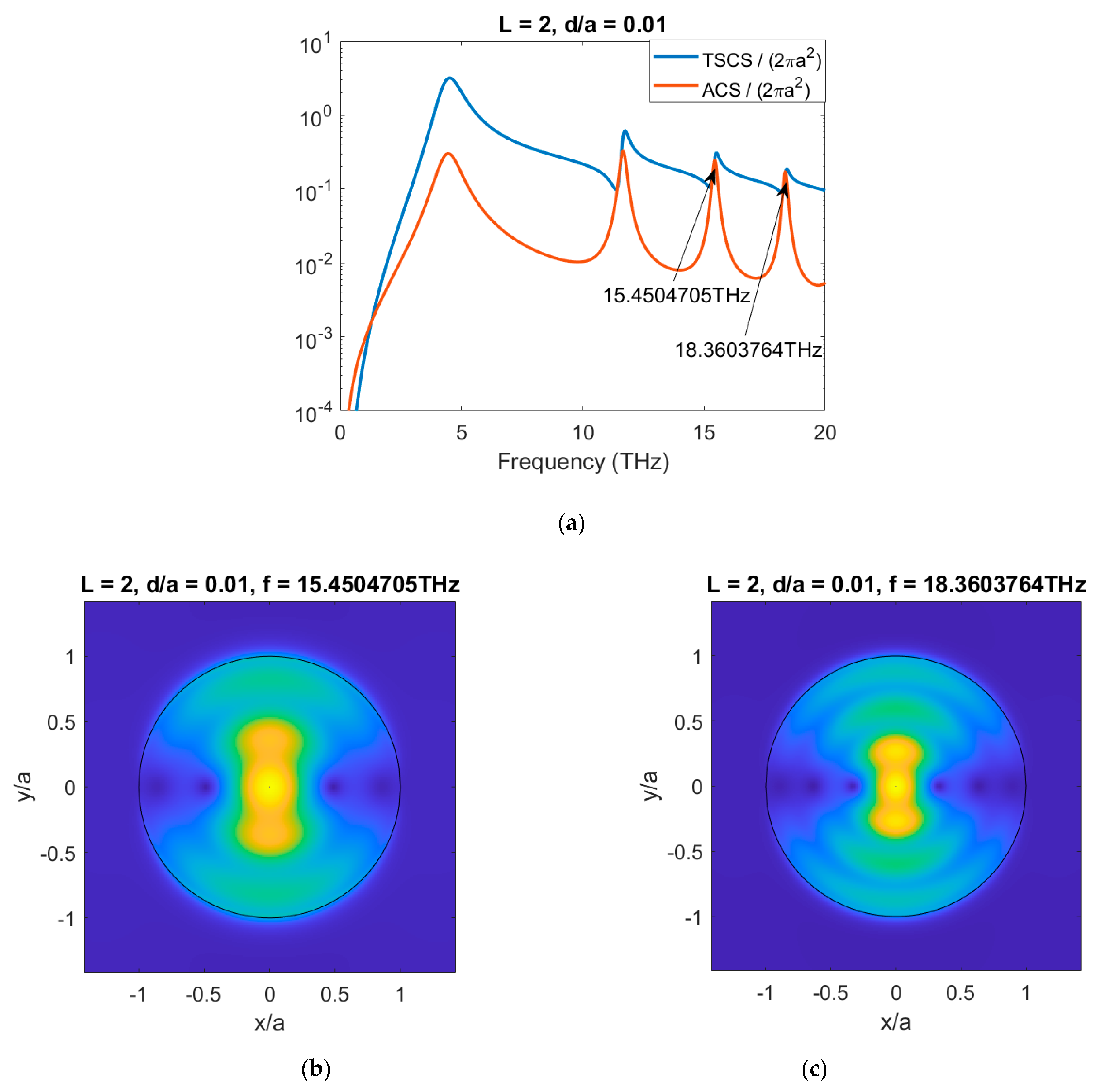
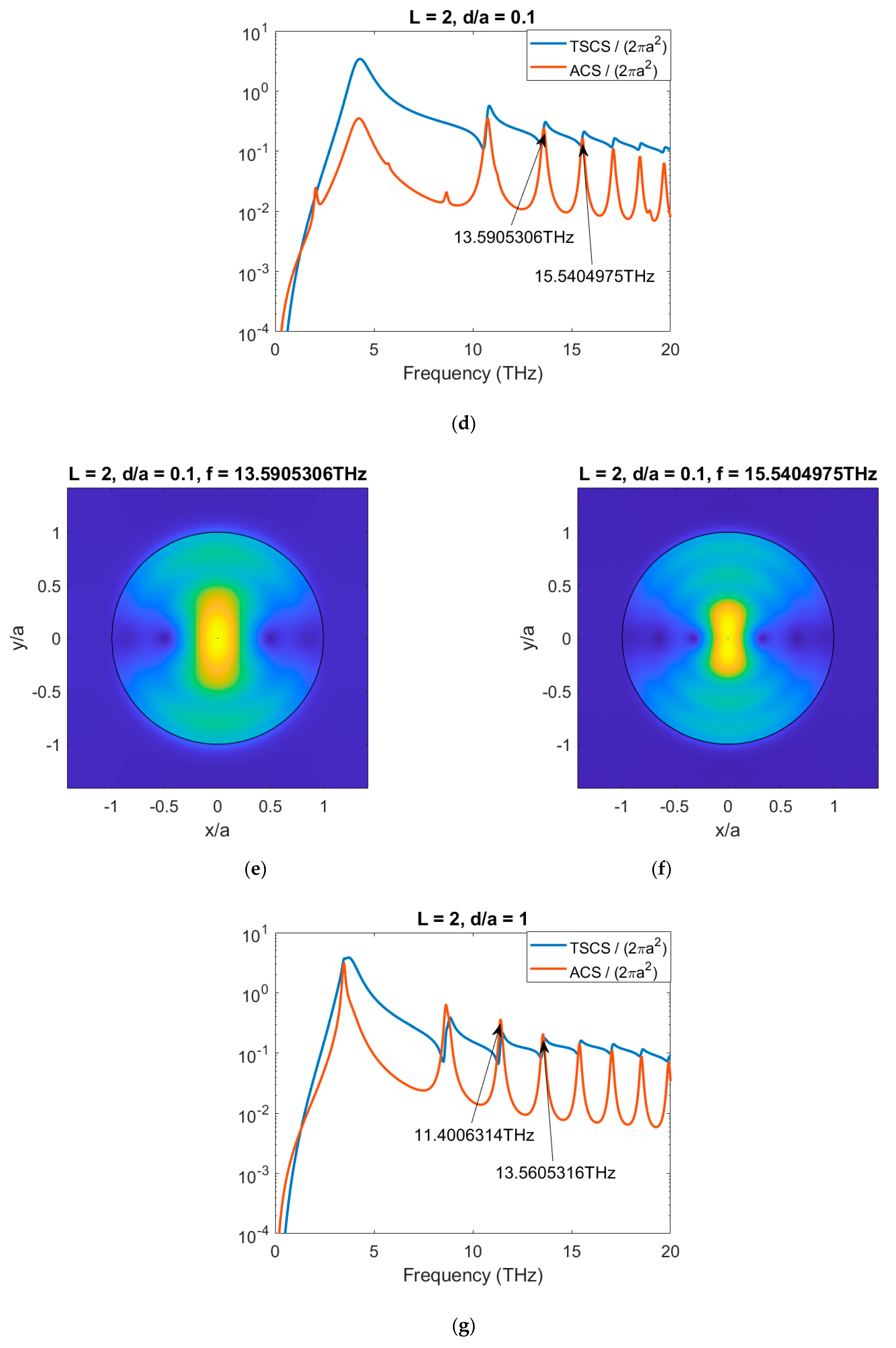
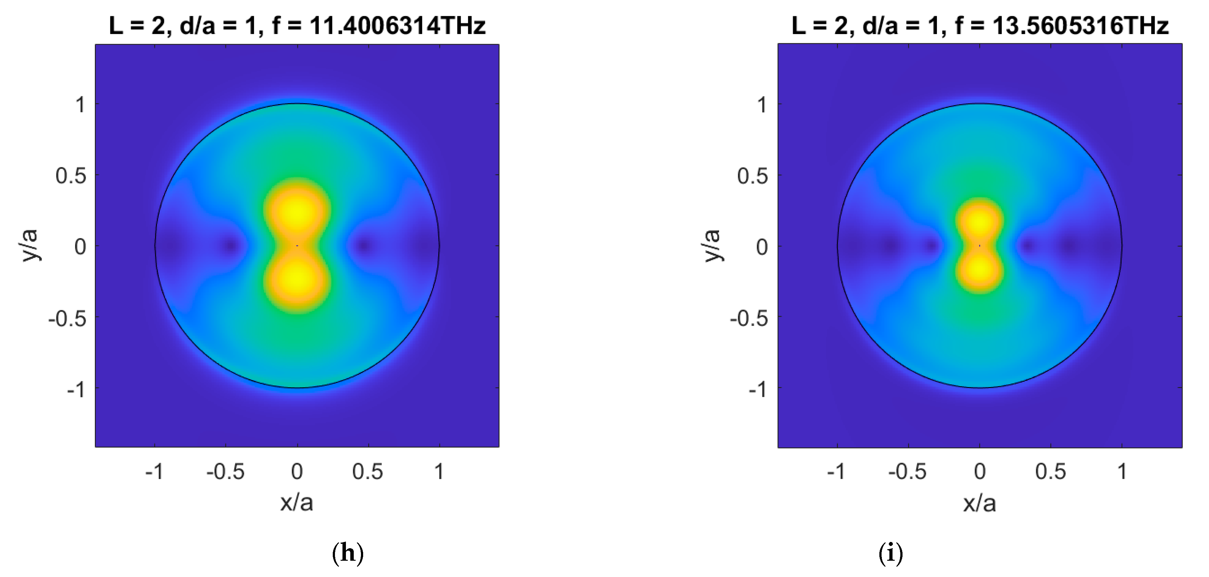
In the first example, we set $L=2$ and show TSCS and ACS for varying values of the frequency and for $\frac{d}{a}=0.01, 0.1, 1$. In Figure 3, the resonance frequencies of the third and fourth SPRs are marked and the near-electric field behavior on the top disk’s plane is shown. As can be clearly seen, the SPR frequencies downshift by increasing the distance between the disks. Indeed, the resonance frequencies associated with the considered modes are, respectively, 15.4504705 THz and 18.3603764 THz for $\frac{d}{a}=0.01$, 13.5905306 THz and 15.5404975 THz for $\frac{d}{a}=0.1$, and 11.4006314 THz and 13.5605316 THz for $\frac{d}{a}=1$. The SPR frequencies are, however, almost the same for $L=2$, $\frac{d}{a}=1$, and $L=1$, which can be interpreted as the case for $L=2$ and $\frac{d}{a}\to +\infty$, thus showing a slight effect of the disks’ coupling for $\frac{d}{a}\ge 1$. To conclude, small new peaks arise for $\frac{d}{a}=0.1$, which are discussed in the next example.

In the second example, TSCS and ACS are provided for varying values of the frequency, for a small with respect to the radius distance between the disks, $\frac{d}{a}=0.01$, and for $L=3, 4, 5$. In those cases, two effects of the disks’ coupling can be observed (see Figure 4). First, the SPR frequencies upshift by increasing the number of the disks. Indeed, the resonance frequency of the third SPR shifts from 15.4504705 THz for $L=2$ (see Figure 3) to 18.2283268 THz for $L=3$, 20.3768854 THz for $L=4$, and 22.0854271 THz for $L=5$. Secondly, new resonances arise, due to the disks’ coupling, identified by small peaks, which upshift by increasing the number of disks. Just for an example, the frequency of the first resonance marked in Figure 4 shifts form 2.8537002 THz for $L=3$, to 3.4242523 THz for $L=4$ and 4.0848799 THz for $L=5$. By examining the near-electric field behavior in the figure, it can be concluded that those resonances are different from the SPRs and resemble the dipole-mode resonances of the dielectric disk [34].

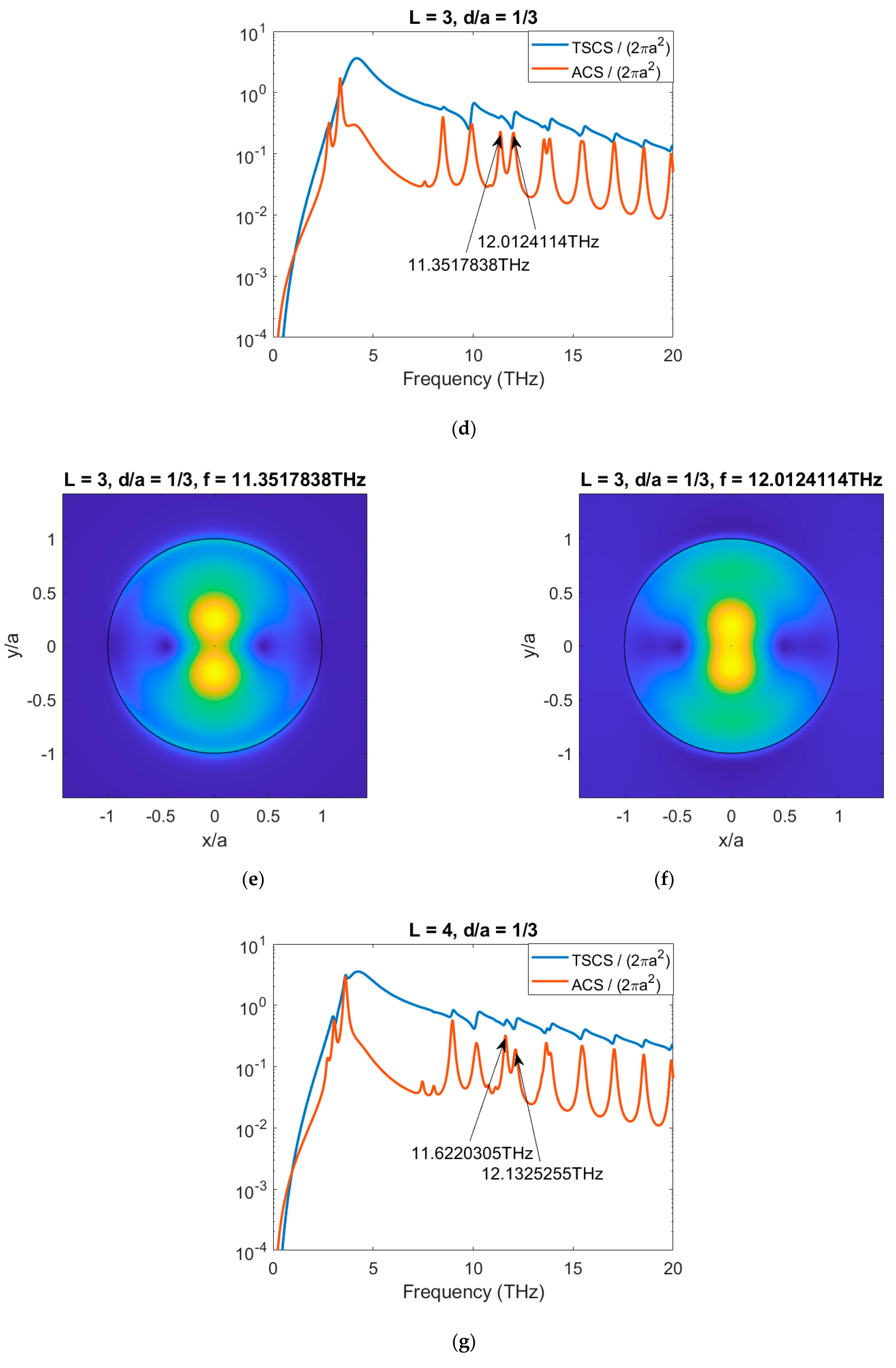
The last example shows another interesting phenomenon associated with the disks’ coupling. For a larger distance between the disks, $\frac{d}{a}=\frac{1}{3}$, the peaks of TSCS and ACS associated with some of the SPRs split, generating two modes with a very similar behavior of the field. In Figure 5, the cases for $L=2, 3, 4$ are considered. The frequencies marked are associated with the same SPR, with two oscillations along the radial direction. The resonance frequency of such a mode for $L=1$ is 11.4008974 THz (see Figure 2) and splits in the resonance frequencies 10.9806450 THz and 11.8206178 THz for $L=2$, 11.3517838 THz and 12.0124114 THz for $L=3$, and 11.6220305 THz and 12.1325255 THz for $L=4$. As usual, the resonance frequencies upshift by increasing the number of disks, but less than in the case for $\frac{d}{a}=0.01$.

6. Conclusions

In this paper, the analysis of the SPRs of a graphene microdisk stack has been carried out by means of an analytical-numerical regularizing technique based on the Helmholtz decomposition and the Galerkin method. The resonance frequencies have been efficiently individuated by searching for the peaks of TSCS and ACS, and the near-electric field behavior for some of the resonances provided. The conducted analysis has shown that, due to the disks’ coupling, the SPR frequencies upshift by increasing the number of disks and by decreasing the distance between the disks, and that new resonances can arise for small with respect to the radius distances between the disks, resembling the dipole-mode resonances of the dielectric disk, while, for larger distances, the SPRs can split.

It is worth observing that, in more realistic situations, graphene disks are components of more complex structures. When the graphene disks lie on dielectric slabs or are parts of thin composite disks, the presented method can be still applied by properly selecting the Green’s function of the problem and/or the boundary conditions. For this reason, those configurations will be the subject of forthcoming papers.