Article

Comparing Charging Management Strategies for a Charging Station in a Parking Area in North Italy

1
Laboratory of Systems and Technologies for Sustainable Mobility, ENEA C.R. Casaccia, Via Anguillarese, 301, 00193 Roma, Italy
2
Solar Thermal, Thermodynamic and Smart Network Division, ENEA C.R. Casaccia, Via Anguillarese, 301, 00193 Roma, Italy
*
Authors to whom correspondence should be addressed.
Future Transp. 2023, 3(2), 684-707; https://doi.org/10.3390/futuretransp3020040
Submission received: 21 February 2023 / Revised: 6 April 2023 / Accepted: 12 May 2023 / Published: 19 May 2023

Abstract

:
Via the analysis of a set of parking and journey information for vehicles traveling to the parking site at the University of Brescia (Italy), we evaluated the possibility of managing the electric recharging of these vehicles, which are hypothesized to be electric. The paper investigates charging optimization techniques that can limit the charge power peaks and distribute the energy demand throughout the day. A cost assessment for an auxiliary system consisting of a photovoltaic energy source (PV) and battery stationary storage (BSS) is also carried out. Optimal power management at the station with PV and BSS is introduced, and the performance of two feedback controllers based on the optimized results is compared with that of a real-time management algorithm in the presence of randomness in charging requests and insolation. The results show that the BSS degradation cost plays a primary role in determining the strategy to adopt to minimize the operating expenditure of a charging station.

1. Introduction

Electric mobility represents a sustainable solution in urban areas thanks to the absence of harmful emissions and noise. It is capable of making the city environment more livable thanks to the reduction in smog, which represents a critical element for health protection [1]. Its sustainability becomes even more evident when we consider the benefits of the lower greenhouse gas emissions that electric vehicles (EVs) have the potential to offer [2], which are linked to the carbon footprint of the electricity production used to charge EVs. Green electricity production represents the optimal solution, and the European Commission proposes the ambitious goal of climate neutrality by 2050 [3]. The greater application of renewable electricity sources (RES) and volatile charging requests will require a transformation of the electricity grid to compensate for the variability of the RES via the greater flexibility of the grid [4], the use of energy storage [5], and different kinds of energy management by the user [6].
The development of the charging infrastructure impacts the electricity grid, posing the problem of the ability to respond to power requests [7]. One way to limit the adverse effects is to integrate the charging infrastructure with storage systems and renewable energy sources [8] that are capable of containing power peaks and withdrawals from the grid via on-site energy production [9]. The presence of energy storage can be beneficial, especially for fast-charge infrastructures [10]. The factors that influence the size of the auxiliary systems and their possible implementation are various, including the available space, the additional cost, the entity of the reduction in the withdrawal from the grid, and the diversity of the storage. The implementation of smart charging strategies is also envisaged as a possible mitigation action [11]. In the present work, we evaluate the problem of dimensioning a charging station at a parking lot of the University of Brescia (Italy) and the optimization of the daily operation on an economic basis. The charging station is equipped with a photovoltaic system (PV) and a battery storage system (BSS). A PV is a good solution for the local production of energy for charging infrastructures in urban areas [12,13]. In addition to the benefits of providing clean energy for recharging electric cars, the coupling between a PV and a charging station equipped with a fixed battery can represent a business model [14].
Charging stations at the workplace are spreading rapidly and represent a valuable charging opportunity [13,15]. The extended parking period allows slow charges and the management of energy flows. The smart management of the charging demand can reduce the impact on the electricity grid, optimize the use of the renewable energy generated [16], and is of fundamental importance in cases in which the recharging infrastructure, possibly equipped with storage, is part of a microgrid [17]. Indeed, although the intermittent photovoltaic production and the uncertainty of the charging demand of electric vehicles can negatively affect the grid stability, the coordinated operation can overcome these problems, potentially reducing energy costs and improving the carbon footprint [18]. In fact, the uncertainty of demand and photovoltaic production are aspects of the charging infrastructure management on which research is focused. As an example, in [19], the authors proposed an offline particle swarm optimization for a prediction layer, and dynamic programming for the online reactive management layer, for fast charging stations. The problem of the dynamic variability of loads in the presence of PV and a BSS and for a distributed network of charging stations has been addressed in [20] using a multi-agent deep reinforcement learning method to avoid the need for a centralized optimal charging management.
Uncertainty about PV production is another element to consider when planning the use of resources. In [21], a charging and discharging power planning algorithm is applied to the case of large charging stations and solved by a chance-constrained programming method. The reported results show that a good level of confidence in insolation predictions allows a considerable reduction in the cost of charging electric vehicles compared to an uncoordinated method. In [22], a real-time energy management algorithm was developed for a charging system in a grid-connected car park equipped with PV based on a fuzzy controller. However, the system does not consider the presence of a BSS.
The present work focuses on the management of power flows in the presence of uncertainty in loads and insolation predictions. The main novelties of the study with respect to the state of the art are as follows:
  • The use of floating car data to determine parking attendance, as well as to estimate consumption.
  • The use of numerical weather prediction (NWP) models for insolation forecasts.
  • The quantification of the economic advantage deriving from optimized management for the forecasts of the previous day compared to real-time management according to the variations between forecasted and actual values for load and insolation.
A schematic representation of the research steps is illustrated in Figure 1.
The paper is organized as follows: Section 2 analyses the data relating to the cars’ journeys that end up at the Brescia University parking lot and the management of requests to the charging infrastructure. An evaluation of the cost-effectiveness of the investment is made for a PV source equipped with a BSS. In Section 3, the daily power flows to the station are studied with the aim of optimizing the use of the BSS based on the forecasts of user influx and insolation, according to an economy criterion. The impact of input variability is studied by comparing the performances of two automatic feedback controllers and a real-time power flow management system. Section 4 presents the conclusions. Appendix A presents an insight into the methodology for weather forecasts.

2. Materials and Methods

The study is based on the analysis of floating car data (FCD) related to a large fleet of private vehicles that are equipped with devices for acquiring GPS positions with a sampling period of about 30 s. FCD were collected over an area covering the province of Brescia (Italy) in March and November 2019 and provided by VEM solution [23]. The top left corner of the FCD extraction rectangle has coordinates (46.63, 9.69) while the bottom right is (45.13, 11.30), and correspond roughly to the area reported in Figure 2.The GPS records include several aspects including an anonymous vehicle identifier, longitude and latitude, a timestamp, the distance between two consecutive traces, the state of the engine, the instantaneous speed, and the quality level of the GPS signal.
From the data set, the records of the journeys ending at the Brescia University car parking are selected. Charging systems for electric vehicles have been installed in the parking area as part of the MoSoRe@Unibs project [24]. The extracted dataset consists of 147 records. Journeys are concentrated on working days, while the number of events over the weekend is scarce (4 arrivals referring to 3 cars). Given the small number of events over the weekend, we focus the analysis on working days. The average number of arrivals registered on weekdays is three cars per day. Figure 3a shows the hourly distribution of the frequency of arrivals. These were gathered from the 7 a.m.–8 a.m. and 1 p.m. time slots, with about 82% of the events occurring within the 1 pm slot. No events are recorded in the 7 p.m.–7 a.m. time slot. Figure 3b shows the average duration of parking events based on the arrival time for working days.
The average duration of the daily stops is 3.9 h. More than 57% of parking events last less than 4 h, with about 81% ending within 7 h. Less than 5% of layovers last 10 h or more. The average duration of the stops is rather limited for the afternoon arrivals (12 a.m.–5 p.m.), while the longest layovers are recorded for the evening hours (6 and 7 p.m.).
The hourly distribution of the average distances traveled, as reported in Figure 4a, shows that these are generally higher for arrivals occurring in the morning than in the afternoon and evening. The distribution of occurrences by journey distances, as reported in Figure 4b, shows that most journeys are cover short distances. Approximately 69% of the trips are within 20 km, and almost 90% are within 40 km.
To evaluate the charging demand of an electric car fleet, and the impact on the charging facility, we suppose that the recorded traces belong to purely electric vehicles (BV). To estimate the consumption of these BVs, we assume that the amount of charge required is proportional to the distance traveled to arrive at the workplace. The routes have been reconstructed from GPS data using a map-matching technique that allows an accurate evaluation of the distances traveled [25]. An estimation of the average consumption for electric cars [26] indicates that the average consumption is 15 kWh/100 km for batteries smaller than 50 kWh and 17 kWh/100 km for larger ones. For the records in the database, we assume that vehicles with average distances traveled equal to or less than 30 km are equipped with smaller batteries and that those with greater average distances are vehicles with batteries larger than 50 kWh. In this way, it is possible to roughly estimate the energy demand at the station as the product of the distance traveled and the average consumption for that battery size.

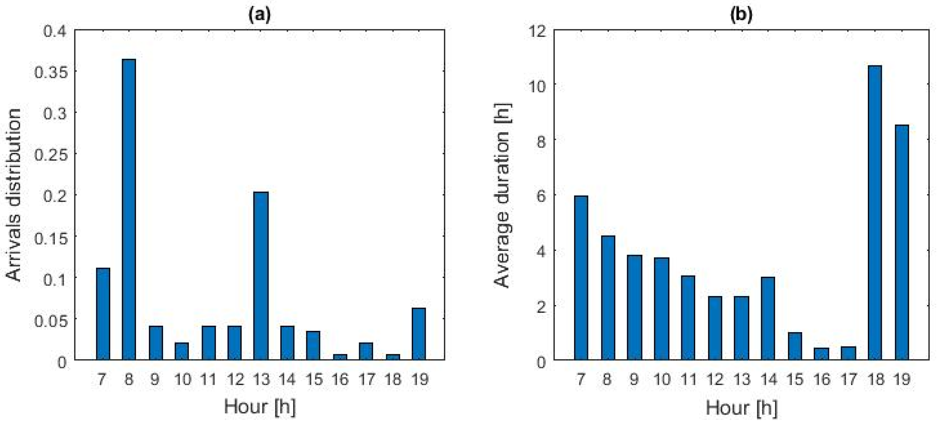
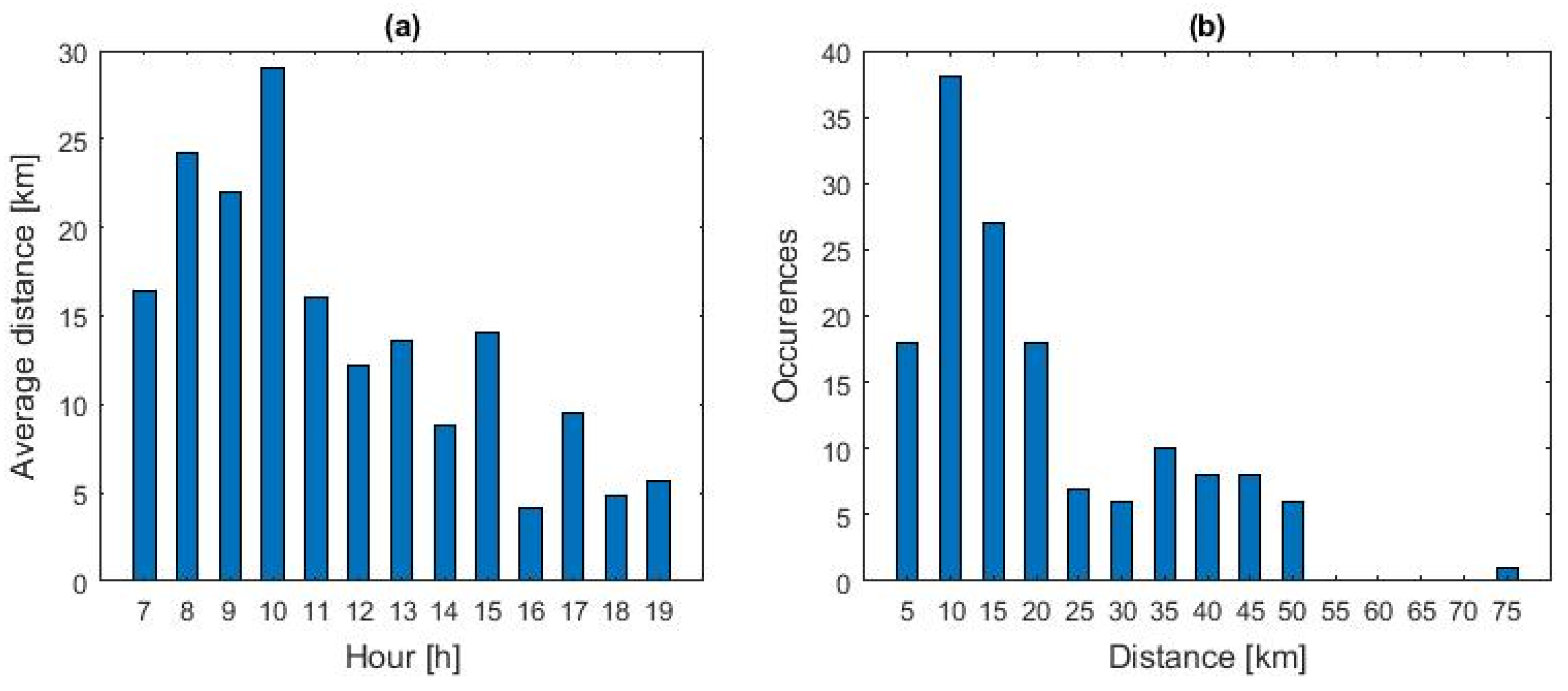
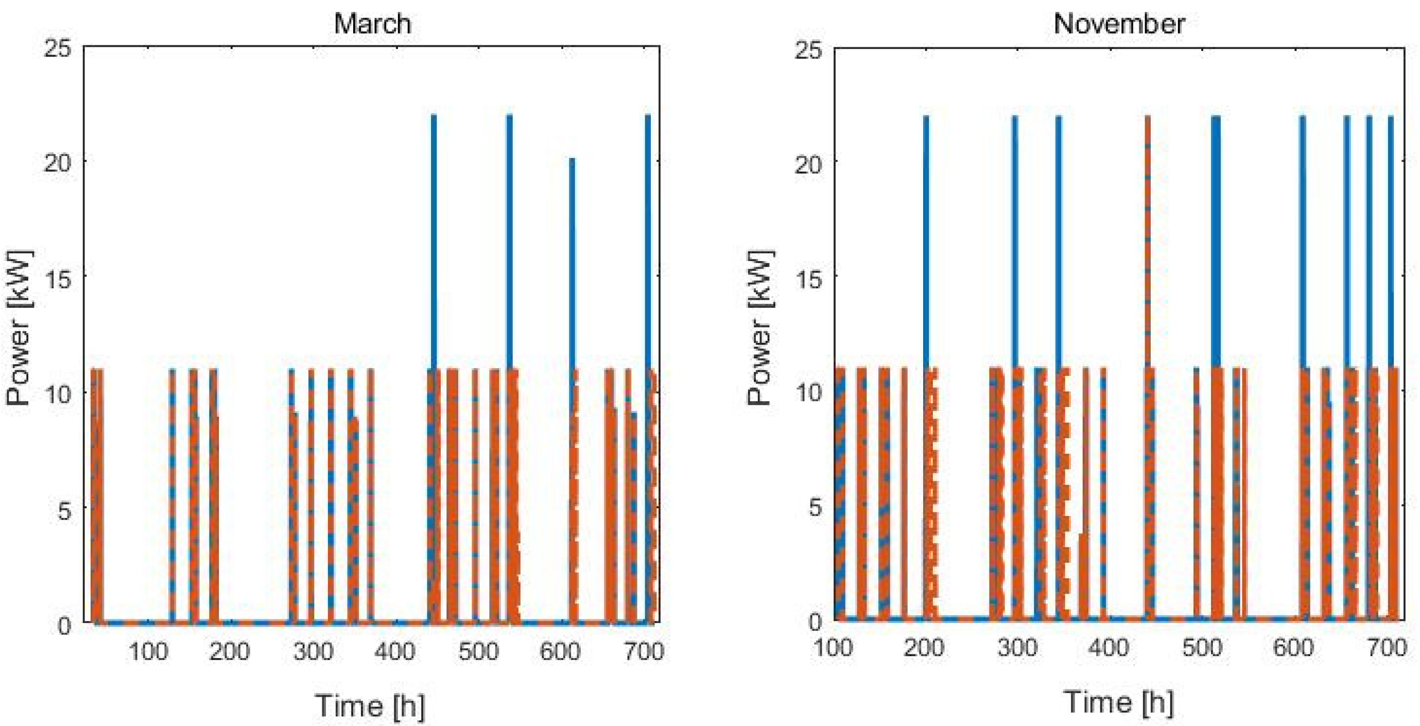
2.1. Load Profiles and Demand Management

The station installed in the car park consists of two 22 kW charging points, with the possibility of using each of them as two 11 kW chargers. The charging station cannot have more than 2 points of 22 kW, 4 of 11 kW, or 1 of 22 kW and 2 of 11 kW occupied simultaneously. We chose to assign 22 kW to large cars that are unable to fully charge the energy used to arrive using the lowest power. Conversely, other users, including all small cars, were assigned 11 kW charging. Not all users may be able to fully recharge the energy used on the journey. A hypothetical charge request to the station is generated from the analysis of the traffic data. The specific power profile depends on the demand management policy. In the following, we compare two possible approaches:
(a)
First-in first-out (FIFO), in which users are served on a first-come first-served basis. There are no constraints on the charging power used in the station.
(b)
Linear optimization, in which the algorithm aims to keep the overall power used at the station below a certain threshold, applying a linear optimization method to modulate the individual charge’s power.
Approach (a) does not require knowledge of the daily arrival schedule but only of the energy required and the parking duration. Conversely, approach (b) requires prior knowledge of arrivals and the stop lengths.
In the FIFO approach, the charge starts as the car arrives at the station if there is an available charger. Otherwise, the EV enters a queue. Charges take place with the power level chosen according to the criteria illustrated above. If the residual dwell time is insufficient to charge all the energy used in the journey, the battery will only be partially filled.
Approach (b) considers the following information on the charging events foreseen during the day: arrival time, duration, required energy, and maximum charge power. The optimization process aims at keeping the overall power absorbed by the station below a given P l i m value, which in principle can vary over time:
f = j = 1 M x j t i P l i m ,         t i N
where N is the number of time intervals into which the analyzed period has been divided, M is the number of vehicles being charged, and x j t i is the power profile for EV j at t i . The constraints are represented by the following system:
0     x j t i     P m a x j ;
i = 1 n x j t i t = E j r e q
Inequality (2) represents a constraint on the minimum and maximum power for the charging event. The former is set to zero since we are not considering the possibility of withdrawing energy from the EV’s battery, while the latter corresponds to the maximum absorbable power. In (3), n is the number of time slots in which the parking time of the j - th EV is divided, t is the length of the time intervals, and E j r e q represents the energy that the j - th EV would have charged during the idle time in absence of modulation. Compliance with this constraint could result in the impossibility of finding solutions to the problem. In this case, it is possible to proceed in two distinct ways:
  • Ignore the violation of the limit power constraint when it is impossible to find a solution to the problem and charge the requested energy.
  • Admit the possibility of not supplying all the energy needed to comply with the power limits at the station.
In the present study, we chose strategy 1. To solve the system, we used the command “solve” of MatLab [27], which utilizes “linprogr” [28] as solver for the linear optimization problem. From the distribution of arrivals, dwell time, and journey lengths, it is possible to create time series of charge requests at the station for an arbitrary number of users. We assumed that the dwell time and the distances traveled both obey Gaussian distributions, for which average values and variances come from the statistical analysis of the original data. We generated N scenarios, each characterized by a time series of arrivals and related energy consumption. Each scenario corresponds to a daily load profile generated by applying approach (b). We use these load profiles as input to determine the effectiveness of the investment for the PV and BSS systems.

2.2. Evaluation of the Cost-Effectiveness of Photovoltaic Sources and Storage

We evaluate the convenience of a charging station integrated with a PV source and a BSS, which represents the most suitable solution for domestic or commercial systems [29,30]. The input data for the evaluation are investment costs of the system components, insolation and average temperature of the installation site, average electricity price, and charge demand.
The net present value (NPV) can be used to determine the optimal size of the PV and the BSS. This method determines the value of future cash flows (positive and negative) generated by a project during its useful life. An investment is profitable when the NPV is positive. The NPV is valued over a time horizon of N years and is a function of the cash flows relating to the investment made, including the interest rate (k). Therefore, it can be expressed as follows:
N P V = t = 1 N F t ( 1 + k ) t I
where:
  • N is the time horizon of the investment in years;
  • F t is the cash flow in the t - th year, calculated as the difference between the cash flows with and without the PV + BSS system;
  • I is the initial investment calculated as the sum of PV and BSS capital expenditure (CAPEX);
  • k is the interest rate fixed at 3%.
From (4), it is possible to establish which size of a system provides the best investment.
Finite values for the efficiency of power converters were used in the analysis. The time horizon of the investment is 15 years, which represents a compromise between the expected duration of a PV system, over 20 years [31], and that of a recharging station, approximately 10–12 years [32,33]. In addition, the replacement of BSS after 7.5 years is considered.
For the evaluation of the investment, we have considered that, according to the European Energy Innovation [34], the cost of a residential photovoltaic system without taxes is about EUR 1.2/Wp. Given an expected reduction in the costs by 2025 [35], the price of photovoltaics in 2022 for residential buildings can be estimated around EUR 1.2/Wp turnkey. We have not included any analysis of the influence of COVID-19 on the price of the PV system. The investment cost of the BSS is estimated at EUR 0.35/Wh for the lithium battery [36,37].
Using the daily curves of power demand at the station, considering the annual average insolation over Brescia and the hourly energy price for the year 2022, we obtain that the optimal size for the PV is about 2.7 kWp, with a storage of about 1.2 kWh. The PV size is rather small due to the low number of daily users (3 cars per day on average), which does not allow a convenient exploitation of the charging facility. Therefore, we analyzed a situation with a doubled number of daily arrivals, using the procedure for determining synthetic charging profiles illustrated in the previous section. Using these curves as input for the determination of the NPV, we obtain that the optimal size is 11 kWp for the PV and 7 kW for the BSS. We reiterate that these values were obtained assuming that the price of electricity and the number of average daily users do not vary throughout the investment period.

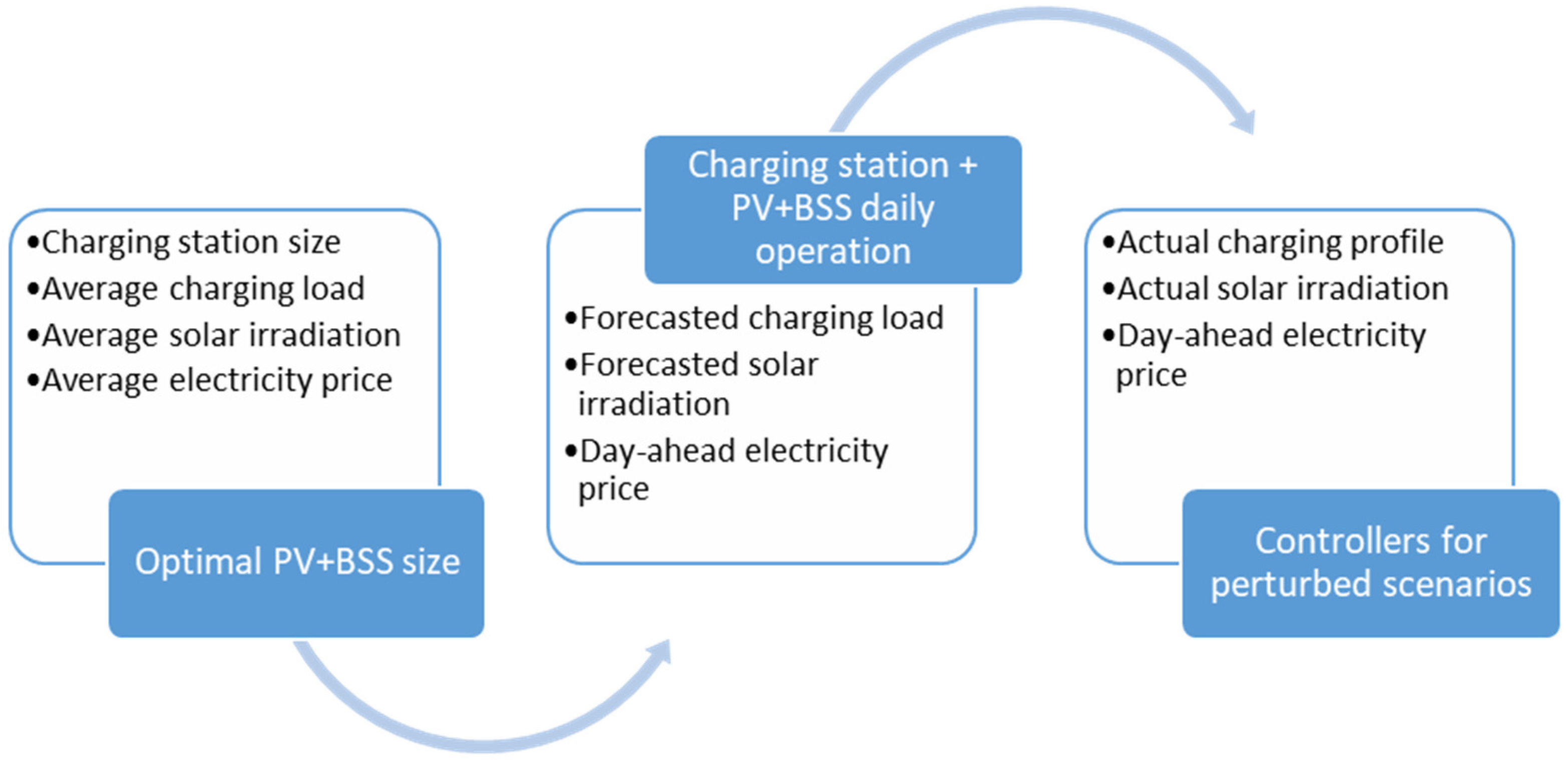
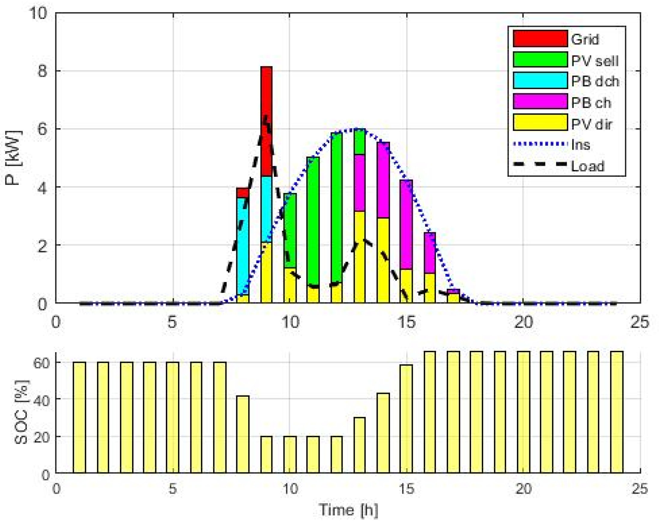
2.3. Optimization of Charging Infrastructure Daily Operation

With a priori knowledge of photovoltaic production, power demand by users, and the hourly price of electricity, it is possible to optimize the use of the BSS in order to minimize the daily cost of the charging infrastructure [38].
In optimizing the daily running costs, the operating costs of the photovoltaic system have not been considered since these are much lower than those of the battery. The degradation of the battery is quantified with reference to a complete cycle, i.e., a cycle with a depth of discharge (DOD) equal to 100% of the capacity, which is given by the total cost of the battery divided by the life span expressed in the number of complete cycles as obtainable from the battery datasheet. Assuming a duration of about 5000 cycles and identifying the operating cost with the average cost of the cells, EUR 0.15/Wh [29], the expenditure for a complete cycle is about EUR 0.03/kWh/cycle. Since the battery usage is not always at DOD = 100%, the cycle cost is “weighted” inversely to its actual DOD.
With this estimate for the battery degradation cost, we can optimize the expected power flows at the charging station based on the forecast for demand and sunshine from the day before. The optimization aims to maximize the exploitation of the photovoltaic production and to optimize the use of the battery, minimizing the following objective function:
min C e = min h = 1 24 ( C r ( h ) P g r i d h t + C d e g ( h ) )
where:
C r ( h ) is the grid energy price at time h [EUR/kWh];
P g r i d h is the power absorbed from the grid during h [W];
t is the time interval considered (1 h);
C d e g ( h ) is the battery degradation cost [EUR].
It is possible to include the possibility of selling the excess PV generation. In this case, (5) becomes
min C e = min h = 1 24 ( C r ( h ) P g r i d h t + C d e g h C s ( h ) P s e l l h t )
where:
C s ( h ) is the price paid for the energy fed into the grid per hour h [EUR /kWh];
P s e l l h is the excess power compared to the demand produced by the PV system and sold to the grid per hour [W].
We used MatLab linear optimization program to solve the problem [28].

3. Results

We apply the optimization procedures described in the previous section to the Brescia use case. In particular, we consider a charging infrastructure located at the University parking area, which is shown in Figure 5.
The charging infrastructure is equipped with an 11 kWp PV and a 7 kWh BSS system. The inputs of the problem are the load curve, generated with the approach described in Section 2.1; the insolation forecast for the incoming day generated by the Weather Research and Forecasting model (WRF); and the day-ahead energy price. The WRF model’s ability to represent the daily insolation consisting of Global Horizontal Irradiance (GHI) is described in detail in Appendix A. PV panels convert the solar insolation to electric power.
For the charge management, we compare the results for the FIFO and linear optimization approaches, as presented in Section 2.1. For the linear optimization approach, we chose to satisfy the charge requests, even if this leads to a violation of the power limit constraint. Figure 6 shows the results of applying the two approaches for the months analyzed. In particular, the limit value set for the station in approach (b) is 11 kW. With the FIFO approach, the power reaches 22 kW in some cases. If approach (b) is applied, the power always remains below the 11 kW limit, except in a single case in November. The reduction in the above-threshold power used with or without optimization is 89% for the month of November and 100% for March.
From the distribution of arrivals, dwell time, and journey lengths, it is possible to create time series of charge requests at the station for an arbitrary number of users. We assumed that the dwell time and the distances traveled both obey Gaussian distributions, for which average values and variances come from the statistical analysis of the original data. We generated N scenarios, each characterized by a time series of arrivals and related energy consumption. Each scenario corresponds to a daily load profile generated by applying approach (b). To each scenario we apply the optimization of the charging infrastructure daily operation reported in Section 2.3 to minimize operational costs.
Figure 7 shows an example of power flow optimization, considering a forecast of insolation for one day of March. The red bars represent the purchased contribution from the grid, the yellow bars represent the portion of power produced by the PV used to meet the demand, cyan represents the power discharged from the batteries, and magenta represents the charged power, while green represents the portion of PV energy sold to the network. The black dashed line is the load, and the blue dotted line represents the insolation. The bottom panel shows the battery state of charge (SOC). In the simulation, the efficiency of the grid converter, the load inverter, and the photovoltaic panels was set equal to 0.9, while for the battery, it was assumed to be 0.85 in charge and discharge.
As can be seen, the photovoltaic system can produce more power than is required by demand for some hours of the day. When this happens, the battery participates in the power exchange by storing part of the energy. Any surplus is available for sale to the grid. The ratio between stored and sold energy depends on the battery degradation costs and the energy purchase price from the grid. We have assumed that the purchase price is proportional by a factor of 0.25 to the sale price, so we expect a greater propensity to sell than to store the renewable energy surplus when the grid energy price is high.

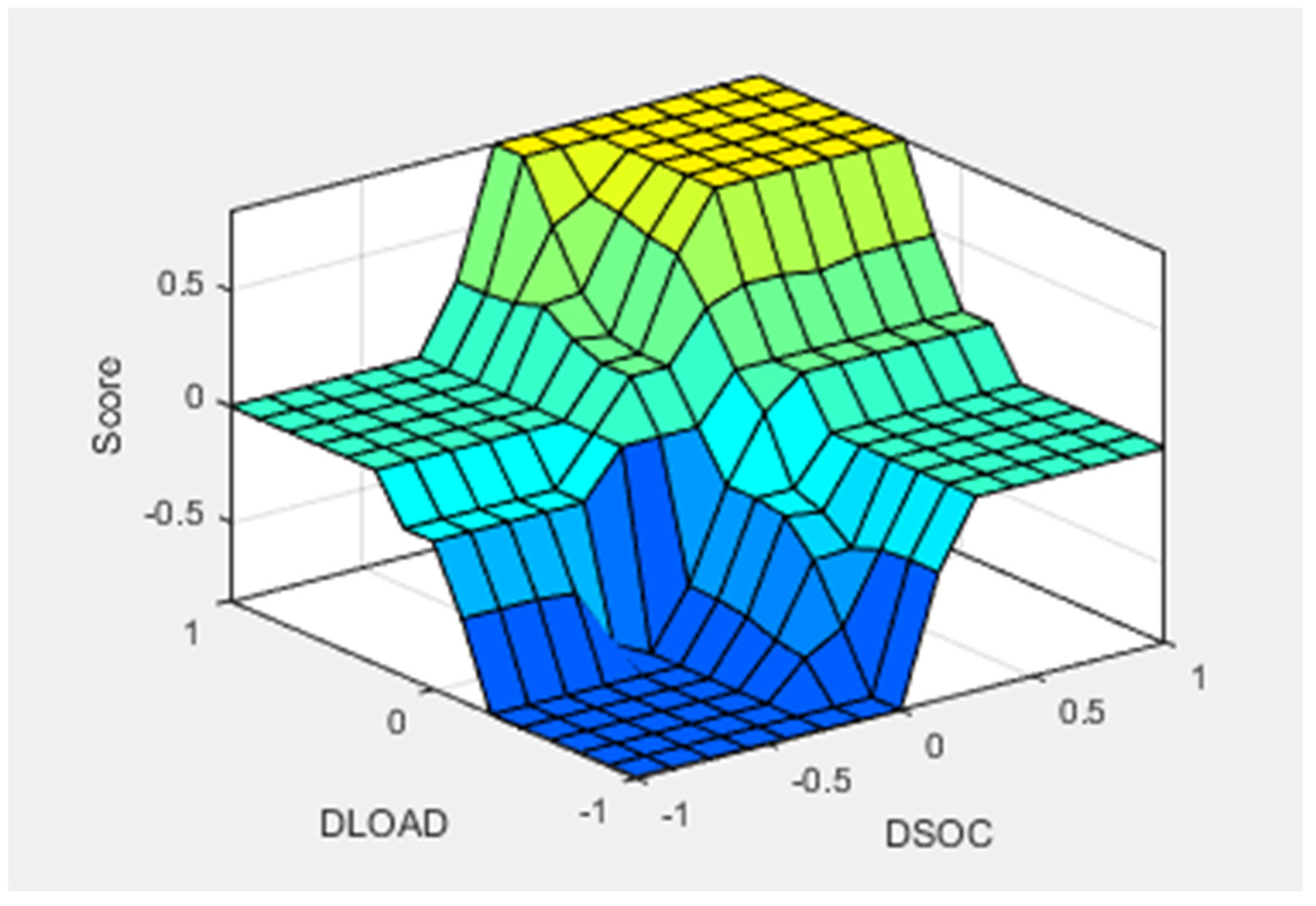
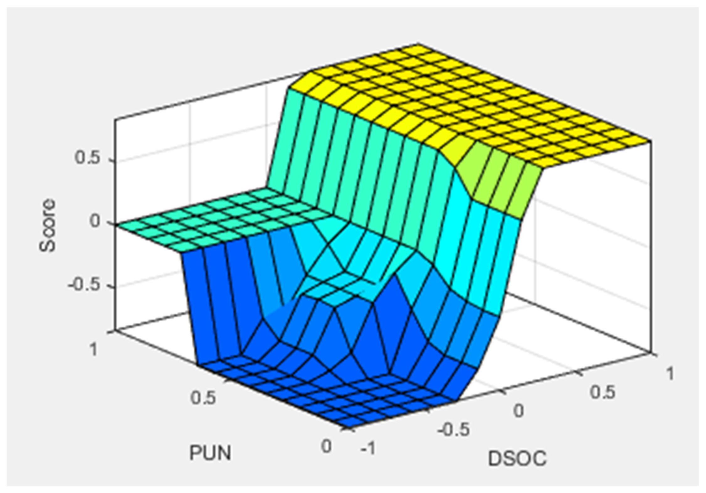
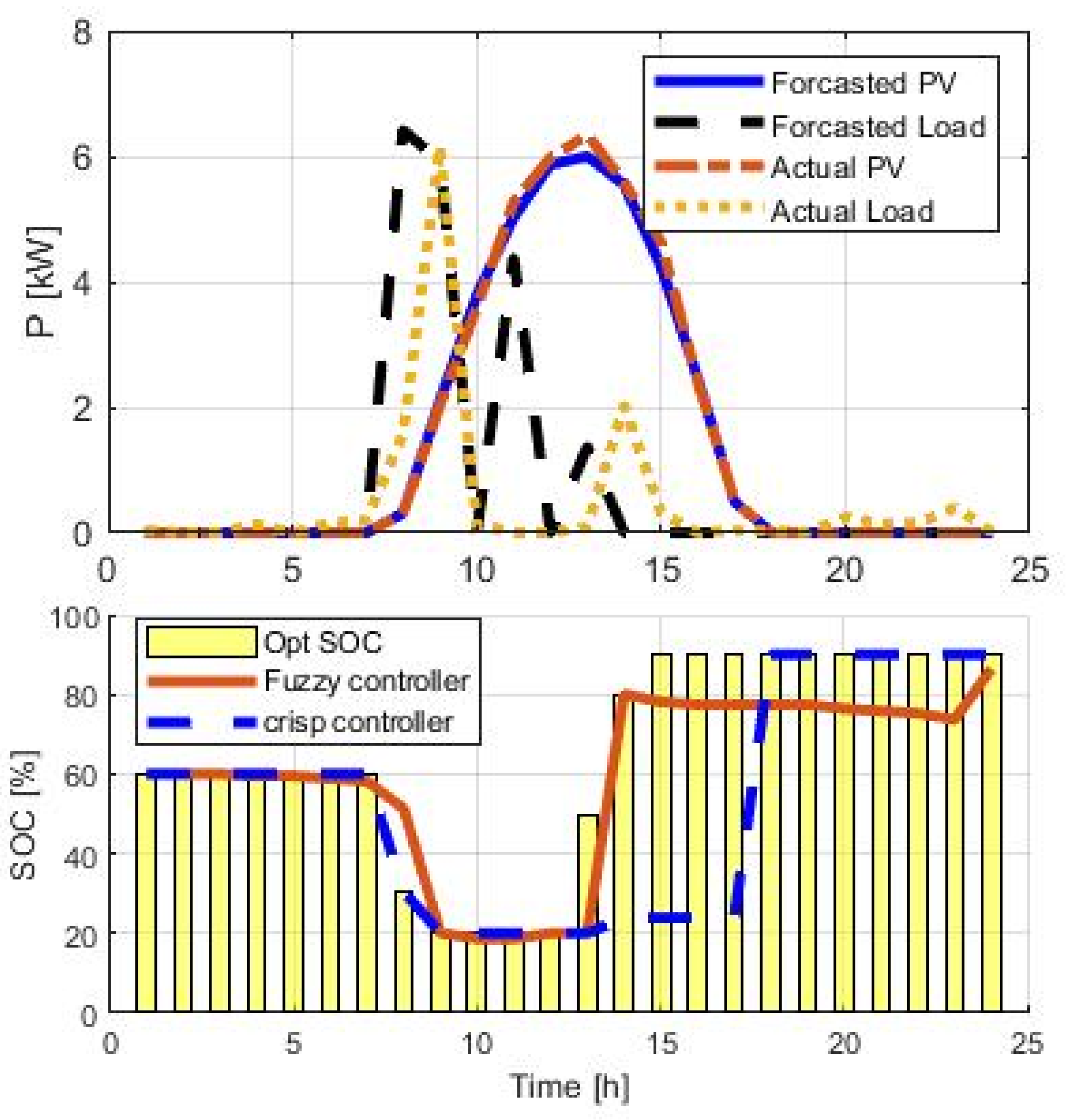
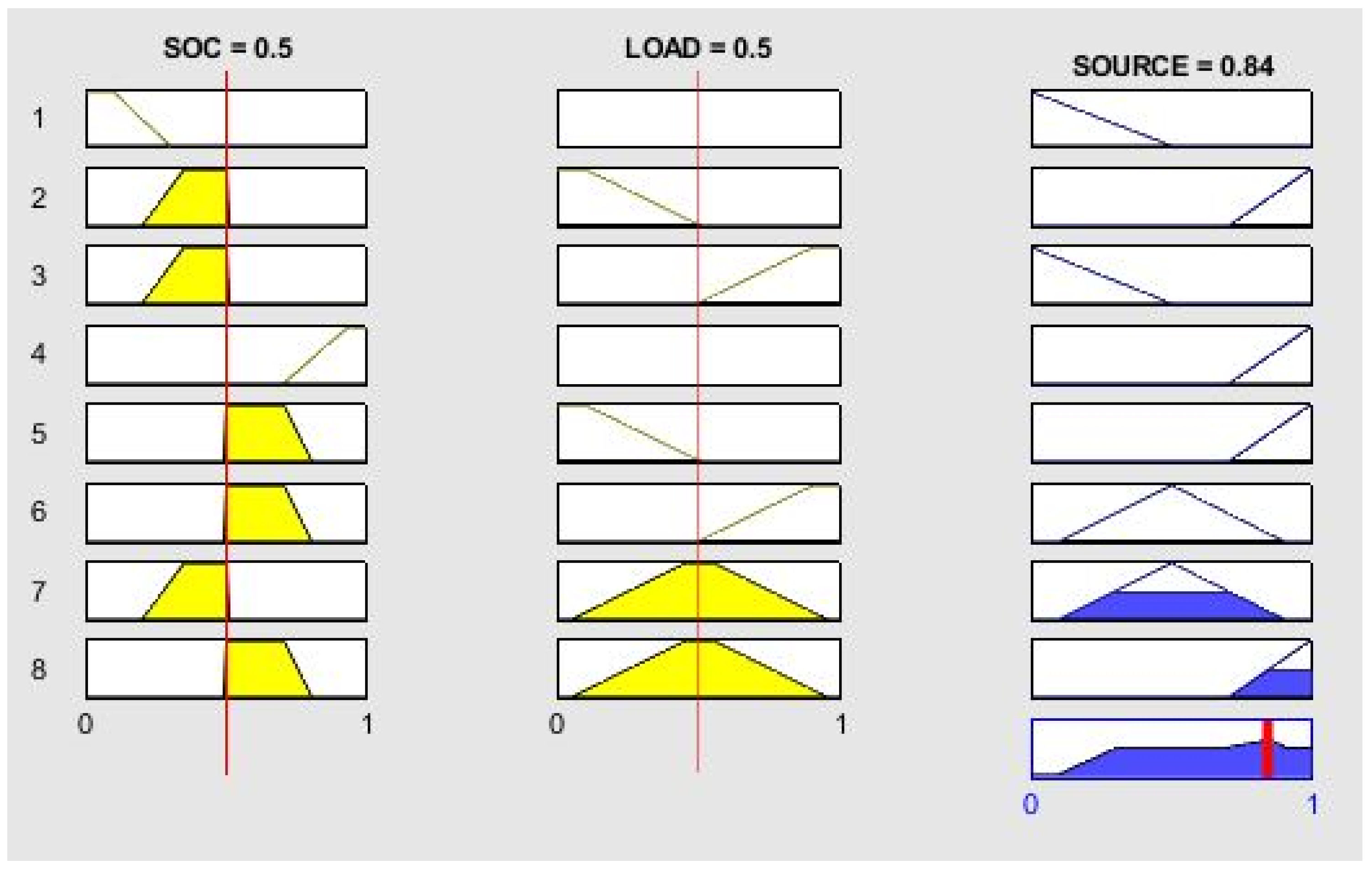
Fuzzy Controller for Optimal SOC Management

The feedback controller (hereinafter “controller”) aims to ensure that the system follows a given behavior, opposing appropriate corrective actions to the deviations due to system perturbations. The fuzzy approach is widely used in this type of problem. Fuzzy logic is a multiple values logic capable of dealing with ambiguous, imprecise, and not exactly defined contexts. These characteristics make it applicable to a wide range of problems. It was introduced in its basic principles in 1965 by Lofti A. Zadeh [39] and formalized and systematized in a definitive way in 1973 [40]. This logic is particularly useful when the problem has multi-valued properties in which there are no specific threshold values (for example, as in the case of describing a person, in which it is necessary to establish whether he is ‘tall’ or ‘short’, ‘fat’ or ‘thin’, and so on). The multi-valued logic is expressed by means of a “membership function” (MF), which represents the degree to which a variable belongs to a property of interest. The MFs are associated with a suitably defined set of implication rules (if–then), creating a functional correspondence between a given input set (also vectorial) x R n and an output set (in the general scalar case) y . This system represents a fuzzy logic system (FLS).
We apply the controller to the battery SOC. We consider the optimal profile for the SOC, obtained based on forecasts of power demand, sunshine, and electricity price for the next day, as illustrated in the previous section. We, therefore, perturb demand and PV production. The controller tries to maintain or restore the SOC to the expected level, implementing the appropriate operational policies that account for the variation in demand, the price of electricity, and the deviation from the expected SOC value. The approach has been implemented in MatLab®, using the Fuzzy Logic Toolbox [41].
Figure 8 and Figure 9 show the three-dimensional curves representing the surface of the rules followed by the model. Figure 8 shows the behavior that considers the variation of the energy demand ‘DLOAD’ (evaluated as the difference between the external demand and the availability from the photovoltaic, normalized between −1 and 1 to the maximum power of the battery), according to the deviation of the actual SOC from the expected one ‘DSOC’ (normalized between −1 and 1). Output values (‘Score’) close to −1 correspond to a greater propensity to recharge the battery; conversely, values close to +1 indicate its propensity to discharge. If the output is zero, no action on the battery is taken, and the corrective actions impact the other components of the system: grid and PV.
Figure 9 shows the surface of the rules for the model that regulates charges from the grid. In addition to the deviation of the SOC, ‘DSOC’, defined as in the previous case, the other input is the value of the price of electricity, ‘PUN’, normalized between 0 (minimum) and 1 (maximum). The output ‘Score’ is defined as in the previous case.
Figure 10 shows an application of the controller for the SOC management, along with the forecasted trend of insolation and demand used in the previous paragraph (scenario 1) and those perturbed (scenario 2). For comparison, we also report the SOC obtained using an on–off logic controller (crisp). The ‘crisp’ controller is a simple algorithm that obeys the following instructions:
  • The battery can be discharged below the optimal SOC to compensate for the insufficiency of renewable energy production.
  • If the energy produced by the PV is greater than the request and the actual SOC is lower than the optimal one, recharge using excess energy until the optimal SOC value is reached.
  • If the actual SOC is lower than the optimal one and there is no PV energy available, recharge until the optimal SOC value is reached if the grid energy price is lower than or equal to the average daily price.
The SOC can vary in the range of [10–90%].
The result shows that both controllers can implement corrective actions to follow the expected SOC trend, with a higher fidelity for the crisp approach.
To test which is the most cost-effective strategy to adopt, we ran a series of 100 simulations on different scenarios for charge demand and PV production. The forecasted load and insolation were perturbed adding a random variation distributed according to a Gaussian distribution with zero mean value. The standard deviation (SD) quantifies the variation amplitude of the variable with respect to its mean value. For the insolation distribution, we set an upper limit equal to the maximum theoretical insolation of the month. Any negative value of the perturbed load is set to zero.
For each simulation run, we calculated the daily costs for the grid energy and battery degradation. We averaged the 100 values obtained and compared the results with the daily expenditure obtained by the optimization algorithm for the expected load and insolation. The difference between optimal and perturbed costs is always positive for two main reasons:
  • The perturbed charging demand is, on average, greater than the expected demand, given that the negative random values are set to zero, which makes the noise distribution skewed toward positive values.
  • The SOC optimized for the forecasted quantities no longer coincides with the optimal trend for the actual situation. Trying to restore its optimal values can be counterproductive.
To quantify the differences of the perturbed and forecasted power profiles, in Table 1, we report the variance percentage between the forecasted and the perturbed energy request, averaged over 10,000 different charging profiles, as a function of the Gaussian deviation of the perturbation. As a comparison, we also report the average percentage difference in PV energy production, which is very close to zero, since, in this case, the corrections to the synthetic profiles only concern violations of the maximum production power and have less of an impact as they are less frequent.
As a measure of the skewness of the difference between perturbed and forecasted distributions, we calculated Pearson’s skewness coefficients s, defined as:
s = 3 ( x x ~ ) / σ
where x is the mean value of the distribution, x ~ is the median, and σ is the standard deviation. We averaged the skewness coefficients over all the 10,000 runs, and the results are reported in Table 2.
As can be seen, the difference between the perturbed and forecasted loads is right-skewed, indicating that the perturbed load is on average greater than the forecasted one. On the other hand, the skewness of the PV production variations is very close to zero.
In all cases, the fuzzy controller has proven to be the best strategy to keep costs down in the presence of perturbations. The average variance percentage of the daily expenditure, with respect to the non-perturbed case, for the fuzzy controller is reported in Table 3 for some SD values. For comparison, the average operating costs obtained with the crisp controller are always 75% higher than the expected costs in the analyzed scenarios of perturbed inputs. This can be attributed to the fact that the crisp controller is more efficient in restoring the SOC optimal trend calculated on the forecasts, which, however, does not minimize the costs in the presence of perturbations.
These results stem from the different management policies for recharging from the grid, which for the crisp controller takes place considering only the presence of a deviation from the ideal SOC and the cost of electricity lower than the average daily price, without considering the extent of these deviations, as occurs in the fuzzy approach.
As noted above, trying to maintain the SOC at an optimal level based on forecasts may not always be the optimal solution in the presence of perturbations. To verify this hypothesis, we compared the result obtained by applying the controllers with that of a ‘real-time’ strategy, which does not contemplate prior knowledge of either the insolation or the arrivals. The inputs of the real-time management program are the daily irradiation, the demand, and the initial battery SOC. The outputs provide the trend of the SOC over time, the energy requested from the grid, and the unused solar energy. The power flow control system maximizes the exploitation of renewable energy, recharging the battery whenever the PV energy is not used directly for the charging demand, until reaching the maximum SOC (90%). The minimum SOC value is 10%.
When the battery needs to be recharged from the grid, the management is entrusted to a fuzzy model, for which the graphical rules representation is reported in Figure 11. The “SOC” input represents the instantaneous state of charge of the battery (between 0 and 1). The “Grid” input is linked to the price of electricity, appropriately scaled between 0 and 1 according to the following rule:
G r i d = ( P U N t P U N m i n ) / ( P U N m a x P U N m i n )
where P U N t is the grid energy price at time t, and P U N m i n and P U N m a x are the minimum and maximum value of the energy price for the day, respectively, as determined on the basis of the reference price of the day-ahead market.
The “score” represents the output. In the present case, the higher the score (close to or equal to 1), the less the battery draws from the network to be recharged. In Figure 11, each row represents one of the 13 rules. The two left columns report the input membership functions; the panels in the right column report the corresponding output membership function. The bottom panel on the right represents the output value.
The fuzzy model rules that regulate the intervention of the battery in the presence of an energy request are shown in Figure 12. The ‘SOC’ input is defined as in the previous model. The ‘LOAD’ is defined as follows:
L O A D = m i n   ( P L P B a t t , 1 )
where P L represents the amount of charging energy that could not be satisfied with PV production. The model tends to keep the SOC around 50%.
The output ‘Source’ represents the attitude of the battery to discharge. Figure 12 depicts the rules. The two left columns represent the input membership functions; the panels in the right column represent the corresponding output membership function. The bottom panel on the right represents the output value.
To evaluate the performance of the ‘real-time’ approach, we report in Table 4 the average cost variation in percentages, with respect to the unperturbed case, for the fuzzy approach without forecasts.
By comparing the results with Table 3, the management of flows via the optimization program and fuzzy controller is the one that minimizes the daily management costs, as long as the forecast variations are contained below a certain threshold. Management with an algorithm that does not consider the forecasts becomes more convenient as the extent of the disturbances increases.
To verify the influence of battery degradation, we repeated the analysis by doubling the degradation costs of the BSS, i.e., EUR 0.3/kWh. The results reported in Table 5 show that when battery degradation costs increase, the use of a controller becomes less convenient than real-time management.
Furthermore, it is interesting to note that the increase in the daily operating cost compared to the optimal case for the fuzzy controller shows a positive correlation with the increasing variability both for the load and PV production (Table 6 and Table 7). For fuzzy real-time management, the correlation between price increase and PV production variability is instead negative, as reported in Table 5, and weaker than the positive correlation with load variation, which is displayed in Table 6.
The results indicate that the performance of the real-time fuzzy model without forecasts depends crucially on the temporal distribution of demand, more so than on the percentage of energy produced from the renewable source.

4. Discussion

In the present work, we have considered a charging station at the Brescia (Italy) University parking lot, and we have verified the economic convenience of coupling with a renewable energy source and a storage system. The charge demand estimation was based on the actual journeys made to reach the car park, detected by a GPS, and recorded in a database. An optimization program manages the charge demand at the station, modulating the power at the single charging points in order to contain the power demand peaks at the station.
Subsequently, the daily power flows at the station equipped with PV and BSS were analyzed. Based on forecasts for demand and solar irradiation, the use of the BSS was optimized based on an economic criterion and maximization of the direct exploitation of the renewable energy produced. By comparing the performance of two feedback controllers, one based on fuzzy logic and the other on crisp logic, we measured the influence that the stochastic variations with respect to the forecasts have on the daily cost of the station. Perturbations always led to an increase in the operational costs. While the crisp controller proved to be more effective in managing SOC correction actions after a perturbation to restore the optimized value, the fuzzy controller gave the best results in terms of cost restraint.
Furthermore, the performances of the controllers have been compared with those of a fuzzy ‘real-time’ management approach, which does not rely on the use of forecasts on demand and PV production. In this case, the cost related to battery degradation plays a decisive role. This comparison is necessary because, in real situations, it is very difficult to have exact forecasts on charging demand and photovoltaic production. In particular, the temporal distribution of the load is subject to multiple factors, which make it difficult to predict its functional shape in advance [42]. In the authors’ opinion, this difficulty will presumably be overcome with the massive diffusion among users of charging station booking apps. The results of the comparison show that as the cost increases it becomes more economical to use a ‘real-time’ approach rather than using a controller to restore the optimal SOC obtained based on forecasts. It is interesting to note that the variation of the operational expenditure shows a negative correlation with the amplitude of the PV production fluctuations for this approach, while it is always positive for the controller because each SOC variation corresponds to a corrective action with a non-zero cost.
The profitability of investing in renewable sources and static storage for charging stations also depends on the expansion of the electric vehicle market. We have not considered it in our NVP analysis as the high degree of uncertainty on the market penetration of the electric carrier requires a cautious analysis to be used in the cost–benefit evaluation [43]. The inclusion of the benefit deriving from the reduction in externalities of conventional transport can influence the results and should be considered in the decision making processes of policy makers [44]. This consideration goes beyond the scope of this work and deserves future study.
These results are useful for defining the most convenient charging station management depending on technological design choices. The analysis of the actual charging data and power flows at the station will make it possible to verify the degree of correctness of the study outcomes and will be the subject of subsequent studies.

Author Contributions

Conceptualization, N.A.; methodology, N.A., G.C. and I.B.; software, N.A.; validation, N.A., G.C. and I.B.; formal analysis, N.A.; investigation, N.A.; resources, N.A.; data curation, N.A.; writing—original draft preparation, N.A., G.C. and I.B.; writing—review and editing, N.A., G.C. and I.B.; visualization, N.A.; supervision, N.A. project administration, N.A.; funding acquisition, N.A. All authors have read and agreed to the published version of the manuscript.

Funding

This research was funded by POR FESR 2014–2022, project MorSoRe@UniBS ID 1180965.

Institutional Review Board Statement

Not applicable.

Informed Consent Statement

Not applicable.

Data Availability Statement

Not applicable.

Conflicts of Interest

The authors declare no conflict of interest. The funders had no role in the design of the study; in the collection, analyses, or interpretation of data; in the writing of the manuscript; or in the decision to publish the results.

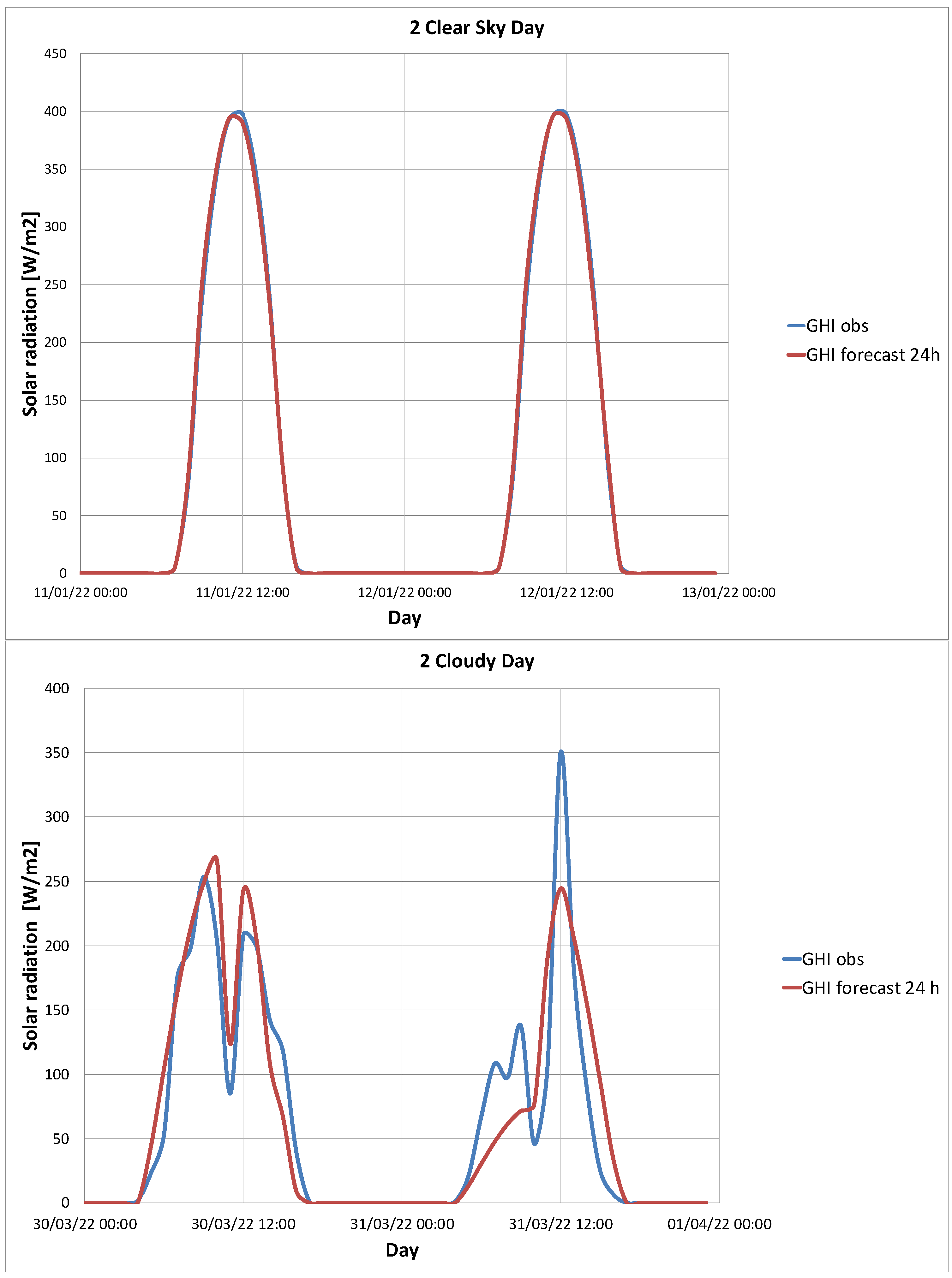
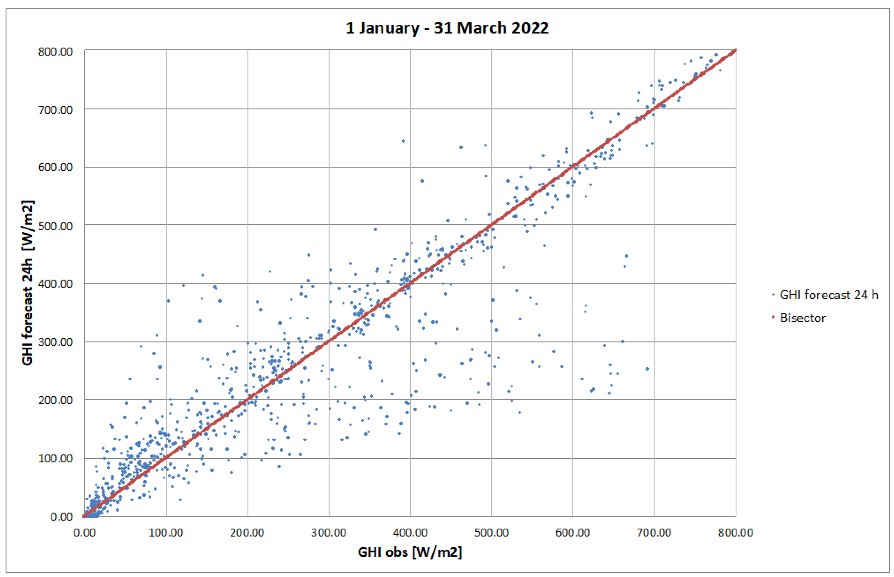
Appendix A. The Weather Research and Forecasting Model (WRF)

The spacious, continuous, and long time series of ground in situ observations are difficult to find. A Numerical Weather Prediction (NWP) model is one of the techniques to obtain continuous and spacious atmospheric data. NWP models use numerical computational techniques to simulate the spatial and temporal differential equations of physical and dynamical interaction between the atmosphere and the ocean onto a desired geographical configuration [45].
These numerical tools, in a good manner, become indispensable for estimating renewable energy. Meteorological forecast models, nowadays, can predict in a good manner the renewable resources for wind farms [46,47], solar power plants (Photovoltaic [48], and Concentrated Solar Power systems [49]). Those models became the governing tool for renewable energy forecasts and the management of the energy systems [50].
In this paper, we used the simulations of the Weather Research and Forecasting model (WRF) [51]. This is a state-of-the-art regional NWP system designed for both atmospheric research and operational forecasting applications. The model is used in a wide range of meteorological applications with different time and horizontal scales from tens of meters to thousands of kilometers. The computational model domain is the entire region of Italy, where grid size is set to 10 × 10 km (151 × 151 grid points) with the center of the computational domain at latitude 41.25° and longitude 13.5°. The vertical resolution of models counts 30 sigma atmospheric levels and 4 soil levels. For the input data in the model, we used the NCEP/NCAR Global Forecast System (GFS) [52] (1° × 1° grid resolution) with four-time daily input. Forecast simulations are run each day up to 48 h starting from 0:00 UTC, in which first hours are considered as the model spin-up. The run outputs are then compared with ground observation data.

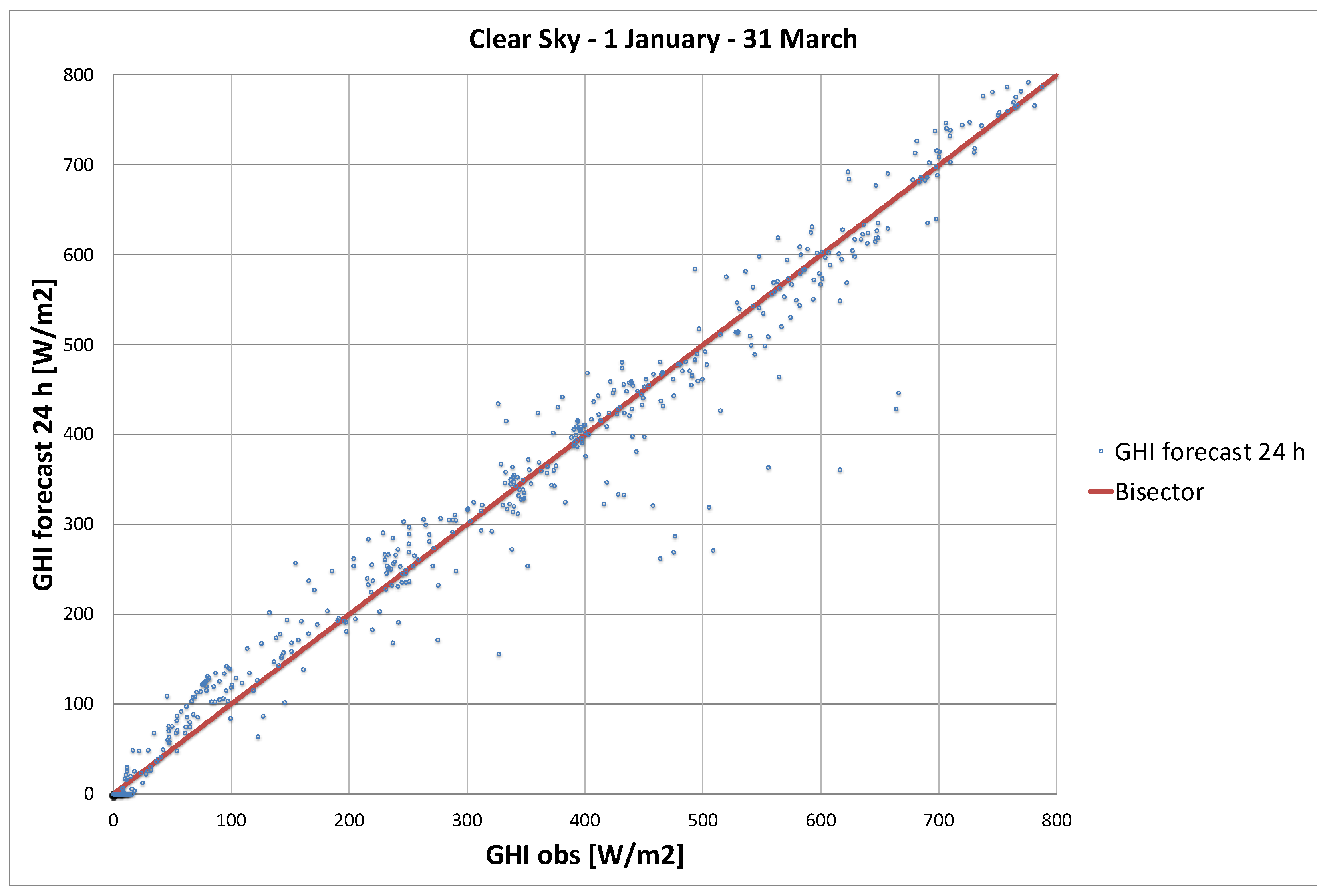
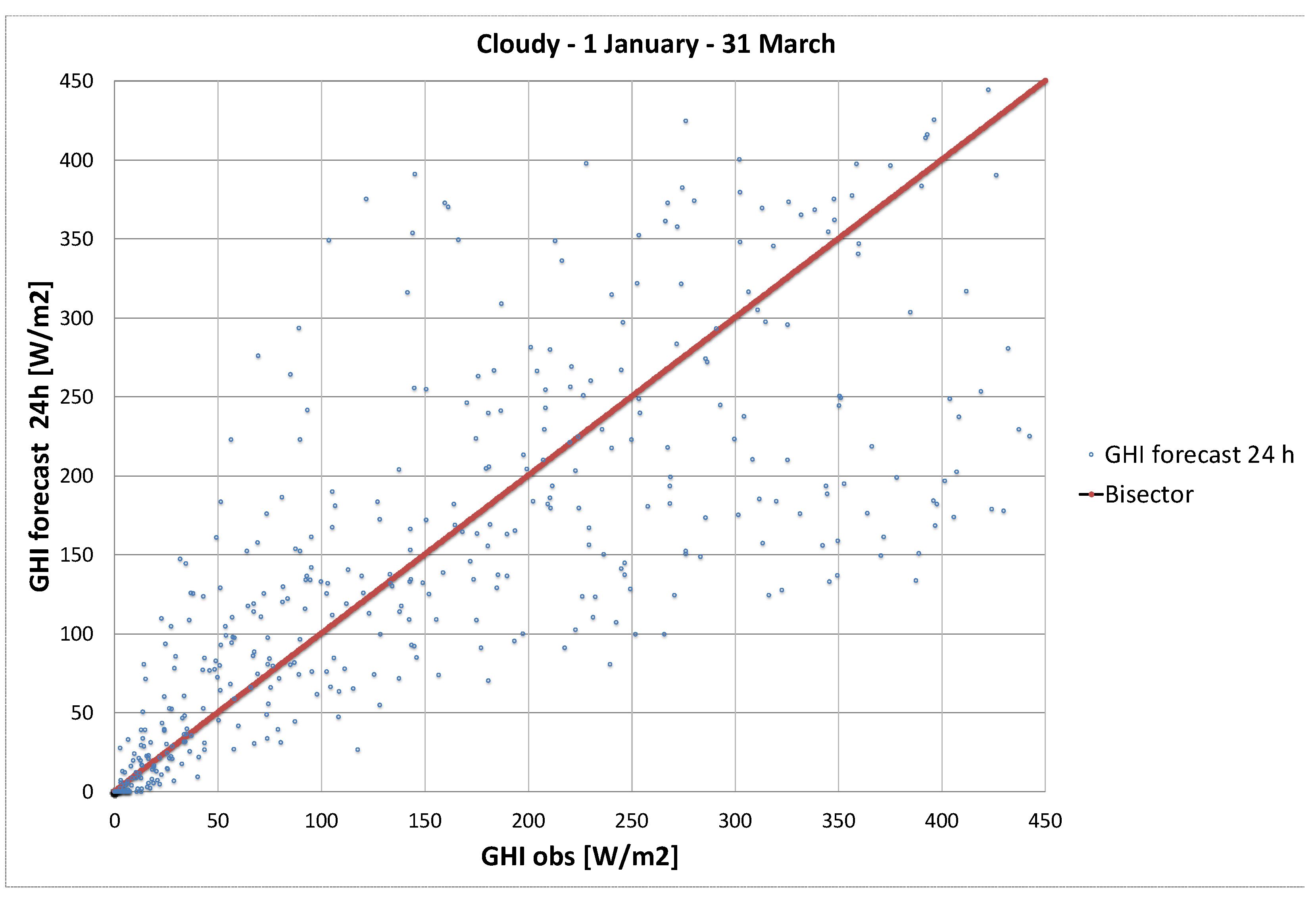
The Skill of WRF Model against the Observation Data

In this section are presented the skill of the WRF model to forecast the Global Horizontal Irradiance (GHI) against observed values at Brescia. The comparative period is from 1 January to 31 March 2022. This period is chosen in consideration of available observation data of Global Horizontal Irradiance being available thanks to the University of Brescia, Department of Information Engineering, eLUX Living Lab.
In Figure A1 are presented the ability of the WRF model to forecast GHI against the observed values for a consecutive 24 h at Brescia. The top panel shows the two days with no cloud conditions (no presence of clouds for the entire sunlight duration), while the bottom panel shows two days with cloudy conditions. The daily cloudy index is defined as the relationship between the sum of the hourly measured GHI against the sum of the hourly extra-atmospheric Global Irradiance, which has values from 0 to 1. Clear sky conditions are considered when the values are higher than 0.65 [53]. It is easy to observe that the model forecasts agree with the GHI values for the clear sky conditions, while for the cloudy conditions, the daily pattern is replicated but the statistics are not representative.
Figure A1. Example forecast (red) and observed (blue) hourly GHI values for clear sky (top) and cloudy days (bottom) of two consecutive days.
Futuretransp 03 00040 g0a1
The next figures present the scatter plots. Figure A2 shows the scatter plot of the 24 h forecasting of GHI compared to the observed values for the entire period. The model has a root mean square error (RMSE) of 59.1 W/m2 for the entire period, considering all sky conditions.
Figure A2. Scatter plot of Global Horizontal Irradiance of 24 h forecasting of all sky conditions against the observed values.
Futuretransp 03 00040 g0a2
In the next step, an additional analysis is presented in which sky conditions are divided in two stages: clear sky and cloudy conditions. Figure A3 presents the scatter plot for selected days with clear sky conditions with an RMSE of only 29.3 W/m2, while on the right are presented the days with cloudy conditions for which the RMSE has an extremely high value of 81.3 W/m2.
Figure A3. Scatter plot of Global Horizontal Irradiance of 24 h forecasting for clear sky conditions (up) and cloudy conditions (bottom) against the observed values.
Futuretransp 03 00040 g0a3aFuturetransp 03 00040 g0a3b

References

  1. Straubinger, A.; Verhoef, E.T.; de Groot, H.L. Going electric: Environmental and Welfare Impacts of Urban Ground and Air Transport. Transp. Res. Part D Transp. Environ. 2022, 102, 103146. [Google Scholar] [CrossRef]
  2. Dillman, K.J.; Árnadóttir, Á.; Heinonen, J.; Czepkiewicz, M.; Davíðsdóttir, B. Review and Meta-Analysis of EVs: Embodied Emissions and Environmental Breakeven. Sustainability 2020, 12, 9390. [Google Scholar] [CrossRef]
  3. European Commission Press Corner. Available online: https://ec.europa.eu/commission/presscorner/detail/en/IP_18_6543 (accessed on 8 February 2023).
  4. Kaushik, E.; Prakash, V.; Mahela, O.P.; Khan, B.; El-Shahat, A.; Abdelaziz, A.Y. Comprehensive Overview of Power System Flexibility during the Scenario of High Penetration of Renewable Energy in Utility Grid. Energies 2022, 15, 516. [Google Scholar] [CrossRef]
  5. Worku, M.Y. Recent Advances in Energy Storage Systems for Renewable Source Grid Integration: A Comprehensive Review. Sustainability 2022, 14, 5985. [Google Scholar] [CrossRef]
  6. Strielkowski, W.; Civín, L.; Tarkhanova, E.; Tvaronavičienė, M.; Petrenko, Y. Renewable Energy in the Sustainable Development of Electrical Power Sector: A Review. Energies 2021, 14, 8240. [Google Scholar] [CrossRef]
  7. Jenn, A.; Highleyman, J. Distribution Grid Impacts Of Electric Vehicles: A California Case Study. iScience 2022, 25, 103686. [Google Scholar] [CrossRef]
  8. Dallinger, D.; Gerda, S.; Wietschel, M. Integration of Intermittent Renewable Power Supply Using Grid-Connected Vehicles—A 2030 Case Study for California and Germany. Appl. Energy 2013, 104, 666–682. [Google Scholar] [CrossRef]
  9. Alkawsi, G.; Baashar, Y.; Abbas, U.D.; Alkahtani, A.A.; Tiong, S.K. Review of Renewable Energy-Based Charging Infrastructure for Electric Vehicles. Appl. Sci. 2021, 11, 3847. [Google Scholar] [CrossRef]
  10. Sbordone, D.; Bertini, I.; Di Pietra, B.; Falvo, M.; Genovese, A.; Martirano, L. EV Fast Charging Stations and Energy Storage Technologies: A Real Implementation in the Smart Micro Grid Paradigm. Electr. Power Syst. Res. 2015, 120, 96–108. [Google Scholar] [CrossRef]
  11. Mancini, E.; Longo, M.; Yaici, W.; Zaninelli, D. Assessment of the Impact of Electric Vehicles on the Design and Effectiveness of Electric Distribution Grid with Distributed Generation. Appl. Sci. 2020, 10, 5125. [Google Scholar] [CrossRef]
  12. Preetham, G.; Shireen, W. Photovoltaic Charging Station for Plug-In Hybrid Electric Vehicles in a Smart Grid Environment. In Proceedings of the IEEE PES Innovative Smart Grid Technologies (ISGT), Washington, DC, USA, 16–20 January 2012; IEEE: Piscataway, NJ, USA, 2012; pp. 1–8. [Google Scholar] [CrossRef]
  13. Chandra, G.R.; Bauer, P.; Zeman, M. System Design for a Solar Powered Electric Vehicle Charging Station For Workplaces. Appl. Energy 2016, 168, 434–443. [Google Scholar] [CrossRef]
  14. Wu, D.; Zeng, H.; Lu, C.; Boulet, B. Two-Stage Energy Management for Office Buildings With Workplace EV Charging and Renewable Energy. IEEE Trans. Transp. Electrif. 2017, 3, 225–237. [Google Scholar] [CrossRef]
  15. Hardman, S.; Jenn, A.; Tal, G.; Axsen, J.; Beard, G.; Daina, N.; Figenbaum, E.; Jakobsson, N.; Jochem, P.; Kinnear, N.; et al. A Review of Consumer Preferences of and Interactions with Electric Vehicle Charging Infrastructure. Transp. Res. Part D Transp. Environ. 2018, 62, 508–523. [Google Scholar] [CrossRef]
  16. Tahara, H.; Urasaki, N.; Senjyu, T.; Funabashi, T. EV Charging Station Using Renewable Energy. In Proceedings of the 2016 IEEE First International Conference on Control, Measurement and Instrumentation (CMI), Kolkata, India, 8–10 January 2016; IEEE: Piscataway, NJ, USA, 2016; pp. 48–52. [Google Scholar] [CrossRef]
  17. Bose, P.; Sivraj, P. Smart Charging Infrastructure for Electric Vehicles in a Charging Station. In Proceedings of the 2020 4th International Conference on Intelligent Computing and Control Systems (ICICCS), Madurai, India, 13–15 May 2020; IEEE: Piscataway, NJ, USA, 2020; pp. 186–192. [Google Scholar] [CrossRef]
  18. Tavakoli, A.; Saha, S.; Arif, M.T.; Haque, E.; Mendis, N.; Oo, A.M. Impacts of Grid Integration of Solar PV and Electric Vehicle on Grid Stability, Power Quality and Energy Economics: A Review. IET Energy Syst. Integr. 2020, 2, 243–260. [Google Scholar] [CrossRef]
  19. Badawy, M.O.; Sozer, Y. Power Flow Management of a Grid Tied PV-Battery System for Electric Vehicles Charging. IEEE Trans. Ind. Appl. 2017, 53, 1347–1357. [Google Scholar] [CrossRef]
  20. Shin, M.; Choi, D.-H.; Kim, J. Cooperative Management for PV/ESS-Enabled Electric Vehicle Charging Stations: A Multiagent Deep Reinforcement Learning Approach. IEEE Trans. Ind. Inform. 2019, 16, 3493–3503. [Google Scholar] [CrossRef]
  21. Li, D.; Zouma, A.; Liao, J.-T.; Yang, H.-T. An Energy Management Strategy with Renewable Energy and Energy Storage System for a Large Electric Vehicle Charging Station. Etransportation 2020, 6, 100076. [Google Scholar] [CrossRef]
  22. Mohamed, A.; Salehi, V.; Ma, T.; Mohammed, O. Real-Time Energy Management Algorithm for Plug-In Hybrid Electric Vehicle Charging Parks Involving Sustainable Energy. IEEE Trans. Sustain. Energy 2014, 5, 577–586. [Google Scholar] [CrossRef]
  23. VEM-Solutions. Available online: https://www.vemsolutions.it (accessed on 20 January 2023).
  24. Available online: https://www.openinnovation.regione.lombardia.it/it/b/38399/infrastrutture-e-servizi-per-la-mobilit-sostenibile-e-resiliente (accessed on 8 February 2023).
  25. Karagulian, F.; Messina, G.; Valenti, G.; Liberto, C.; Carapellucci, F. A Simplified Map-Matching Algorithm for Floating Car Data. In Lecture Notes in Networks and Systems; Springer Science and Business Media Deutschland GmbH: Berlin/Heidelberg, Germany, 2021; Volume 227, pp. 711–720. [Google Scholar]
  26. Available online: https://www.newsauto.it/notizie/auto-elettrica-quanto-costa-ricaricare-e-quanto-consuma-costo-corrente-energia-elettrica-ev-2020-243194/#foto-42 (accessed on 8 February 2023).
  27. Available online: https://it.mathworks.com/help/symbolic/sym.solve.html (accessed on 8 February 2023).
  28. Available online: https://www.mathworks.com/help/optim/ug/linprog.html (accessed on 8 February 2023).
  29. IRENA. Electricity Storage and Renewables: Costs and Markets to 2030. Ottobre. 2017. Available online: https://www.irena.org/publications/2017/Oct/Electricity-storage-and-renewables-costs-and-markets (accessed on 8 February 2023).
  30. Figgener, J.; Stenzel, P.; Kairies, K.-P.; Linßen, J.; Haberschusz, D.; Wessels, O.; Angenendt, G.; Robinius, M.; Stolten, D.; Sauer, D.U. The Development of Stationary Battery Storage Systems in Germany—A Market Review. J. Energy Storage 2020, 29, 101153. [Google Scholar] [CrossRef]
  31. Available online: https://www.forbes.com/home-improvement/solar/how-long-do-solar-panels-last/ (accessed on 20 January 2023).
  32. Available online: https://www.beny.com/ev-charger-and-charging-station-maintenance/ (accessed on 20 January 2023).
  33. Available online: https://www.gny.com/products/electric-vehicle-charging-stations (accessed on 20 January 2023).
  34. Available online: http://www.europeanenergyinnovation.eu/Articles/Winter-2016/Costs-and-Economics-of-Electricity-from-Residential-PV-Systems-in-Europe (accessed on 22 February 2020).
  35. Vartiainen, E.; Masson, G.; Breyer, C.; Moser, D.; Román Medina, E. Impact of Weighted Average Cost of Capital, Capital Expenditure, and Other Parameters on Future Utility-scale PV Levelised Cost of Electricity. Prog. Photovolt. Res. Appl. 2020, 28, 439–453. [Google Scholar] [CrossRef]
  36. Battery Energy Storage White Paper, SUSCHEM. 2018. Available online: https://www.suschem.org/publications (accessed on 11 September 2020).
  37. Mongird, K.; Viswanathan, V.V.; Balducci, P.J.; Alam MJ, E.; Fotedar, V.; Koritarov, V.S.; Hadjerioua, B. Energy Storage Technology and Cost Characterization Report. United States. 2019. Available online: https://energystorage.pnnl.gov/pdf/PNNL-28866.pdf (accessed on 8 February 2023).
  38. Andrenacci, N.; Di Monaco, M.; Tomasso, G. Influence of Battery Aging on the Operation of a Charging Infrastructure. Energies 2022, 15, 9588. [Google Scholar] [CrossRef]
  39. Lofti, A.Z. Fuzzy sets and systems. In System Theory; Fox, J., Ed.; Polytechnic Press: Brooklyn, NY, USA, 1965; pp. 29–39. [Google Scholar]
  40. Zadeh, L.A. Outline of a new approach to the analysis of complex systems and decision processes. IEEE Trans. Syst. Man Cybern. 1973, 1, 28–44. [Google Scholar] [CrossRef]
  41. Available online: https://www.mathworks.com/help/fuzzy/index.html?s_tid=CRUX_lftnav (accessed on 8 February 2023).
  42. Van Geenhuizen, M.; Nijkamp, P. Coping with uncertainty: An expedition into the field of new transport technology. Transp. Plan. Technol. 2003, 26, 449–467. [Google Scholar] [CrossRef]
  43. Gnann, T.; Plötz, P.; Kühn, A.; Wietschel, M. Modelling market diffusion of electric vehicles with real world driving data—German market and policy options. Transp. Res. Part A: Policy Pract. 2015, 77, 95–112. [Google Scholar] [CrossRef]
  44. Cavallaro, F.; Nocera, S. Are transport policies and economic appraisal aligned in evaluating road externalities? Transp. Res. Part D Transp. Environ. 2022, 106, 103266. [Google Scholar] [CrossRef]
  45. Available online: https://glossary.ametsoc.org/wiki/Welcome (accessed on 8 February 2023).
  46. Available online: https://www.climate.gov/maps-data/climate-data-primer/predicting-climate/climate-models (accessed on 8 February 2023).
  47. Balog, I.; Ruti, P.M.; Tobin, I.; Armenio, V.; Vautard, R. A Numerical Approach for Planning Offshore Wind Farms from Regional to Local Scales over the Mediterranean. Renew. Energy 2016, 85, 395–405. [Google Scholar] [CrossRef]
  48. Tobin, I.; Vautard, R.; Balog, I.; Bréon, F.-M.; Jerez, S.; Ruti, P.M.; Thais, F.; Vrac, M.; Yiou, P. Assessing Climate Change Impacts on European Wind Energy from ENSEMBLES High-Resolution Climate Projections. Clim. Chang. 2015, 128, 99–112. [Google Scholar] [CrossRef]
  49. Balog, I.; Fuoco, D.; Mendicino, G.; Senatore, A.; Caputo, G.; Spinelli, F.; Lepore, M.; Franconiero, D.; Mautone, P.; Oliviero, M. Previsione di Producibilità e Carico, Rapporto Tecnico—D5.3, Modelli Previsionali di Producibilita: Ambiti Applicativi, Rapporto Tecnico di Ricerca Industriale D5.3a. Available online: http://www.comesto.eu/wp-content/uploads/2022/12/ComESto-D5.3a-Modelli-previsionali-di-producibilita%CC%80.pdf (accessed on 8 February 2023).
  50. Giaconia, A.; Iaquaniello, G.; Metwally, A.A.; Caputo, G.; Balog, I. Experimental Demonstration and Analysis of a CSP Plant with Molten Salt Heat Transfer Fluid in Parabolic Troughs. Sol. Energy 2020, 211, 622–632. [Google Scholar] [CrossRef]
  51. Best Practices Handbook for the Collection and Use of Solar Resource Data for Solar Energy Applications: Third Edition. Available online: https://iea-pvps.org/key-topics/best-practices-handbook-for-the-collection-and-use-of-solar-resource-data-for-solar-energy-applications-third-edition/ (accessed on 8 February 2023).
  52. WRF Community. Weather Research and Forecasting (WRF) Model, UCAR/NCAR. 2000. Available online: https://www.mmm.ucar.edu/models/wrf (accessed on 8 February 2023).
  53. Balog, I.; Caputo, G.; Iatauro, D.; Signoretti, P.; Spinelli, F. Downscaling of Hourly Climate Data for the Assessment of Building Energy Performance. Sustainability 2023, 15, 2762. [Google Scholar] [CrossRef]
Figure 1. Diagram of the proposed workflow.
Futuretransp 03 00040 g001
Figure 2. Province of Brescia and metropolitan area (in red) where GPS data have been collected by VEM solution [23].
Futuretransp 03 00040 g002
Figure 3. (a) Hourly distribution of arrivals at the car park and (b) hourly distribution of the average stop durations.
Futuretransp 03 00040 g003
Figure 4. (a) Distribution of average distances traveled by cars by arrival time; (b) distribution of occurrences by distance traveled.
Futuretransp 03 00040 g004
Figure 5. Satellite image of the Faculty of Engineering of the University of Brescia. The red box delimits the parking area.
Futuretransp 03 00040 g005
Figure 6. Total power required at the charging infrastructure with FIFO approach (blue) and applying linear optimization (red, dashed). Right: March; left: November.
Futuretransp 03 00040 g006
Figure 7. Hourly power flows for the load profiles at the station considering the typical insolation of March.
Futuretransp 03 00040 g007
Figure 8. Rule surface for the fuzzy model that controls the change in demand. Input: ‘DLOAD’; ‘DSOC’. Output: ‘Score’.
Futuretransp 03 00040 g008
Figure 9. Rule surface for the fuzzy model that controls grid charging based on electricity cost.
Futuretransp 03 00040 g009
Figure 10. Comparison of system responses following an input perturbation. Top panel: Predicted (blue, dotted) and actual (blue, dotted) insolation and SOC questions adjusted to actual conditions by fuzzy controller (orange solid line) and linear controller (dashed line).
Futuretransp 03 00040 g010
Figure 11. Fuzzy model representation of the 13 rules used to charge from the grid. From left to right, membership functions are reported for the SOC input, the Grid input, and the Score output. Bottom right panel: output score.
Futuretransp 03 00040 g011
Figure 12. Representation of the 8 fuzzy model rules for battery discharge. From left to right, membership functions are reported for the SOC input, Grid input, and Score output. Bottom right panel: output score.
Futuretransp 03 00040 g012
Table 1. Average variance percentage among forecasted and perturbed PV production and load demand over 10,000 perturbed insolation and charge requests for different values of the Gaussian deviation.
Gaussian Standard Deviation0.010.050.100.50
Average ΔPV (%)−0.0034−0.0010.010.064
Average Δload (%)0.351.83.517
Table 2. Average Pearson skewness coefficient for the difference between perturbed and forecasted load and PV production, as a function of the standard deviation of the perturbed quantities.
Gaussian Standard Deviation0.010.050.100.50
skewness ΔPV0.0004−0.0007−0.018−0.0013
skewness Δload1.161.161.151.16
Table 3. Comparison of average daily cost increase (variance percentage %) of perturbed scenario versus optimal forecast for different deviations for the fuzzy controller.
Fuzzy Controller
Standard Deviation PV
Standard Deviation Load0.010.050.10.5
0.0120.02%23.41%24.88%36.13%
0.0519.28%22.48%24.32%37.04%
0.120.76%22.76%27.78%37.73%
0.531.54%30.78%33.11%43.58%
Table 4. Comparison of the average daily cost increase (variance percentage %) for real-time fuzzy management versus the optimal forecast for different levels of insolation and demand perturbation.
Fuzzy Real-Time
Standard Deviation PV
Standard Deviation Load0.010.050.10.5
0.0122.41%22.25%22.03%22.43%
0.0524.97%23.59%24.42%23.71%
0.125.00%24.84%24.50%23.98%
0.533.42%32.58%33.82%31.26%
Table 5. Comparison of the average daily cost increase (variance percentage %) for fuzzy controller and real-time fuzzy management versus the optimal forecast for different levels of insolation and demand perturbation, with battery degradation costs of EUR 0.3 /kWh.
Fuzzy Controller
Standard Deviation PV
Standard Deviation Load0.010.050.10.5
0.0126.73%29.09%32.62%45.80%
0.0524.27%29.73%31.41%45.13%
0.124.65%28.63%32.45%46.22%
0.537.51%37.95%40.27%53.38%
Fuzzy Real-Time
Standard Deviation PV
Standard Deviation Load0.010.050.10.5
0.0125.29%25.32%26.10%24.56%
0.0525.19%26.55%25.25%24.99%
0.127.04%26.66%26.70%26.03%
0.535.36%34.96%35.55%34.59%
Table 6. Correlation coefficient among cost variation and PV production variation for fuzzy controller and real-time approach for different levels of load perturbation.
ΔLoad0.010.050.10.5
Δcost/DPV correlation
Fuzzy controller
0.990.980.981.00
Δcost/ΔPV correlation
Fuzzy real-time
−0.20−0.52−0.95−0.85
Table 7. Correlation coefficient among cost variation and load variation for fuzzy controller and real-time approach for different levels of PV perturbation.
ΔLoad0.010.050.10.5
Δcost/DPV correlation
Fuzzy controller
0.950.970.980.99
Δcost/ΔPV correlation
Fuzzy real-time
1.001.000.991.00
Disclaimer/Publisher’s Note: The statements, opinions and data contained in all publications are solely those of the individual author(s) and contributor(s) and not of MDPI and/or the editor(s). MDPI and/or the editor(s) disclaim responsibility for any injury to people or property resulting from any ideas, methods, instructions or products referred to in the content.

