Article

Estimation of Transfer Time from Multimodal Transit Services in the Paris Region

1
Laboratoire Ville Mobilité Transport (LVMT), Ecole des Ponts ParisTech, Université Gustave Eiffel, 77420 Champs-sur-Marne, France
2
Centre International de Recherche sur l’Environnement et le Développement (CIRED), Ecole des Ponts ParisTech, 94736 Nogent-sur-Marne, France
*
Author to whom correspondence should be addressed.
Future Transp. 2022, 2(4), 886-901; https://doi.org/10.3390/futuretransp2040049
Submission received: 16 September 2022 / Revised: 11 October 2022 / Accepted: 24 October 2022 / Published: 1 November 2022

Abstract

:
A reliable public transport system is beneficial for people traveling in the metropolitan area. Transfer time in multimodal transit networks has been highlighted as one of the measures of public transport service quality. In this paper, we propose a novel method to estimate the passengers’ transfer time between the transit modes (i.e., train, metro, and bus) based on the 2018 Household Travel Survey in the Paris region, France. The transit trips with a single transit leg are primarily studied, wherein average wait time and mode speeds are estimated through an integrated linear regression model. Based on these inferences, transfer time is deduced within the trips of multiple transit legs. The decomposition procedure of journey time facilitates the estimation of the time components, and reveals the transfer variability in mode, time, and space. From the results, we find that the transfer to the railway modes, especially to the metro, costs less time on average than the transfer to the bus in the study area. The transfer patterns in the morning and evening peak hours are different regarding the transfer duration and locations. Lastly, the results’ reliability, method scalability, and potential applications are discussed in detail.

1. Introduction

The rapidly developing transportation systems have changed people’s travel behaviors, especially in metropolitan areas. Many transport agencies attempt to develop sustainable public transport systems, which give a promising solution for the problems of traffic congestion and air pollution. In order to make public transport more attractive, the main measure is the improvement of public transport service quality, e.g., transit reliability.
In transit systems, transportation characteristics in terms of mode speeds and service frequency are spatio-temporally different. Transit operators put considerable effort into improving reliable services via timetable adjustment, network optimization, and infrastructure investments. Passengers are considerably attracted to multimodal (or intermodal) public transport due to its advantages on safety, affordability, environmental impact, etc. [1]. The major concern may refer to the travel time variability (TTV), which has been defined as the time variance for vehicles traveling similar trips, of either the inter-vehicle, inter-period, or inter-day type [2]. Previous studies suggested splitting transit journey time into separate components, assuming the independence of these components, i.e., access time, wait time, in-vehicle time, transfer time, and egress time [3,4]. The reliability of public transport is sensitive to the variability in the time components [4]. This variability is mainly affected by service frequency (or headway) [5] and a range of other variables, such as temporal factors, infrastructure, and passenger demographics [6,7]. Among the journey components, the impact of transfers on the reliability of multimodal transit systems has been highlighted in the literature [6,8,9,10,11]. In general, a transfer is defined as the changing act between modes or between services of the same mode. The concept may include a pure transfer (e.g., walking from a bus station to a train platform) and an incidental activity transfer (e.g., buying a newspaper) [1].
In the literature, there are abundant studies on the estimation of transit travel time distributions (TTDs), aiming to represent network conditions and get insights on the TTV. The TTDs are mainly related to two forms: (1) normal, and (2) skewed, e.g., lognormal or gamma distribution [12,13]. It is said that the decrease in temporal aggregation tends to increase the normality of travel time distributions [12]. This evidence holds the potential to model the linear regression relationship between travel time and explanatory variables. In recent years, many studies have conducted TTV analyses and measured the reliability of transit systems [4,7,14]. For example, the authors of [7] proposed a method to estimate passenger waiting time at transit stations and analyzed the effects of influential variables with a multivariate regression model.
There is very limited literature on the estimation of transfer time distribution between two transit modes. Existing studies took advantages of transit smart card data to identify the transfers and estimate the time spent, according to the tap-in and tap-out times of transit modes [1,11,15,16]. Seaborn et al. [1] established three levels of maximum-elapsed-time thresholds to identify the transfers between the bus and metro systems in London, using smart card data. The thresholds’ estimation did not distinguish the impacts from time and space dimensions. Normally, transfer time includes walking time for a transfer and waiting time at the platform. However, many studies only estimated one of these two components and only a few considered them together. Eltved et al. [6] estimated the walking time distributions from bus stops to train platforms based on a matching of smart card data and automatic vehicle location data. They found that the passengers’ walking speeds and the passengers who engage in activities during the transfer have impacts on the walking time estimation. Sun and Xu, in their work [3], distinguished the O-D metro trips with or without transfers for the wait time estimation at platforms. The platform elapsed time—PET (a generalized platform wait time)—was inferred from the trips without transfers, while the platform elapsed transfer time (i.e., interchange wait time) was inferred based on the trips with transfers, as well as on the previously deduced PET. Our study is inspired by this stage-based procedure. Wahaballa et al. [16] estimated the platform waiting time distribution in London’s underground network, using passive smart card data. Afterward, the same authors in [11] estimated the distribution of transfer time between bus stops and rail stations, using the stochastic frontier model. Both the walking time and waiting time distributions were presented. From the literature review, on one hand, a large amount of studies have used smart card data for the estimation of travel time or time components, and the study of socio-economic relationships is rarely mentioned, due to this kind of information being lacking. On the other hand, to the best of our knowledge, there are no studies using the household travel survey (HTS) dataset, which includes both the users’ mobility and their socio-economic information, for the estimation of different time components.
From the HTS without any information of time components, how to infer average wait time and in-vehicle time for a transit mode? Does the transfer time between two transit modes have spatio-temporal differences? To answer these questions, this paper proposes an integrated model framework to estimate the passengers’ average waiting time, transit mode speeds, and transfer time in the transit system of the Paris region, based on the 2018 HTS. The basic trip-level information (such as departure/arrival times, trip O/D locations, and purposes) and stage-level information (such as stage start/end locations and travel modes within a trip) are available in the survey. However, like many other large-scale HTSs, there is no further information on the time components at the stage level. Therefore, our study will handle this challenging issue, especially for the estimation of transfer time between two transit modes or lines.
The remainder of the paper is organized as follows. Section 2 introduces the study area of the Paris region and the transit data preparation. Section 3 introduces the method, including the linear regression model and the transfer time estimation based on the multi-stage transit trips. Section 4 presents the results of average wait time and mode speeds, and provides evidence of transit network performance in terms of transfer time in different time periods and territorial spaces. The topics on data accuracy, model extension, and applications are discussed in Section 5. Finally, Section 6 provides the main conclusions and highlights our future work.

2. Study Area and Data Preparation

2.1. Transit Networks in the Paris Region

In France, the Paris region (also called Île-de-France) includes the city of Paris and its suburbs (i.e., inner ring and outer ring). About 12.3 million inhabitants resided in this region in 2020 [17]. In Table 1, we see that the city of Paris and the inner ring have a relatively high population density, where 6% of the regional territory accommodates more than 55% of the regional population. The population density even reaches 20,400 hab/km2 in Paris, and about 31% of the total jobs are offered there.
This strongly monocentric pattern of urbanization is supported by the start-like transportation network, especially by the powerful public transport network, see Figure 1. As of 2018, the transit services were provided by a variety of sub-modes: there were 16 metro lines (mainly in the city of Paris), 15 regional rail lines (including Regional Express Railways (RER) and other “Transilien” lines), 9 tramway lines spanning the inner ring, together with more than 1400 bus lines. The investment of public transport is currently further accelerated with the Grand Paris Express Plan, which consists of the development of new automated metro lines going through the suburbs by 2035.

2.2. Data Preparation Based on the 2018 HTS

The HTS in the Paris region (“Enquête Globale Transport” in French, abbr. EGT) has been conducted every 10 years or so. From the recent official report of the 2018 HTS [18], it is uncovered that about 43 million trips (after expansion with sample weights) are made by regional people on an average working day, out of which 34.4% of trips are made by car, 21.9% by transit modes, 39.9% by walking only, 1.9% by cycling, 1.0% by motorized two-wheeler, and 0.9% by other modes (scooters, taxi, and vehicle-for-hire, etc.). More information on the data structure and mobility analysis can be found in [19].
The 2018 HTS corresponds to the first survey stage of the H2020 HTS, and it covers the period from January 2018 to June 2019 before the COVID-19 outbreak in France. The sample contains 5143 households, with a total of 11,492 individuals. After filtering out about 9.8% of the respondents who were out of the range from 5 to 74 years of age and who had no trips on the surveyed day, the filtered dataset includes 7051 individuals in 3927 households generating 28,873 trips.
As aforementioned, one trip may include multiple modal stages. The trip dataset and trip-stage dataset are both available from the survey and they are jointly studied here. In Table 2, the proportional trip frequency is calculated, regarding the six modalities in number of stages per trip. The simple trips with only one stage comprise 63.1%, and the trips of multiple stages comprise 36.9%.
In the survey, the trip mode is identified by the main transport mode with the longest distance among all trip stages. For simplification, we categorize three transit modes after the mode aggregation: train (RER + Transilien), metro (subway + tramway), and bus. For further analysis on mode speeds, the mode of bus is divided into two sub-modes: bus_urb (i.e., bus in the urban area—the city of Paris and inner ring) and bus_sub (i.e., bus in the suburban area—outer ring), according to the bus start/end locations in the region.
The studied dataset of transit trips is prepared by the following four procedures. First, the trips (including transit and other modal trips) with a number of stages (i.e., modality) corresponding to three, four, and five are chosen (≥6 is ignored with less than 1% of the total trips), as a transit trip includes at least three modal stages: access, transit ride, and egress. Second, the complete transit trips are selected on the condition of owning the information on the stages of the aforementioned transit modes. Third, we specifically select the transit trips with the first access and the last egress stages performed by walking and with a walking distance for each stage of less than 1.5 km (accounting for about 97%, see Figure 2). This filtering rule considers the phenomenon of high frequency of transit connection by walking in the region. Fourth, we remove the outliers of transit trips and keep data intervals between the 2.5th and 97.5th percentiles, regarding the transit trip distances and durations. Finally, there remain 6050 transit trips for the study. For the following different purposes, we segment the transit trips into three groups: Modality 3 denoting the trip of “walk access—PT (public transport)—walk egress” for average wait time and transit speed estimation; Modality 4 of “walk access—PT—PT—walk egress” for transfer time estimation; and Modality 5 of “walk access—PT—PT—PT—walk egress” for transfer time validation.
Since public transport offers different service frequencies in different times of the day, the temporal factor is taken into account to estimate the average wait time to board the first transit mode. In Figure 3, the distribution of the selected transit trips depicts the volume patterns in the four time periods: AM peak (6 h to 10 h), inter peak (10 h to 16 h), PM peak (16 h to 20 h), and off peak (other hours). The same time periods are also defined in the recent regional transport model—MODUS 3.1 [20].

3. Method

Here, we distinguish two types of transit trips to infer the journey time components. The first type of 3-stage trips with one transit leg are used to estimate average platform wait time and transit speeds (followed by in-vehicle time), using an integrated linear regression model. The second type of 4-stage trips with two transit legs are used to infer the transfer time between two transit modes or lines using the estimated wait time and speeds from the first step. Before introducing the inference procedure above, we establish the following assumptions.

3.1. Assumptions

  • The declaration errors of the journey time in the survey are unbiased;
  • The average wait time (only after the walk access stage) and transit mode speeds estimated from the 3-stage transit trips are also representative for all transit trips;
  • The average wait time is highly relevant to the factors of time periods and transit modes, and the mode speeds are distinguished in the urban and suburban areas only for the road transit (i.e., the bus), rather than the railway transit;
  • The transfer time is defined as the time spent from alighting one transit mode (or line) to boarding another transit mode (or line) in the same trip. The transfer time estimated from the 4-stage transit trips is also applicable to other multi-stage transit trips.

3.2. Linear Regression Model Based on 3-Stage Transit Trips

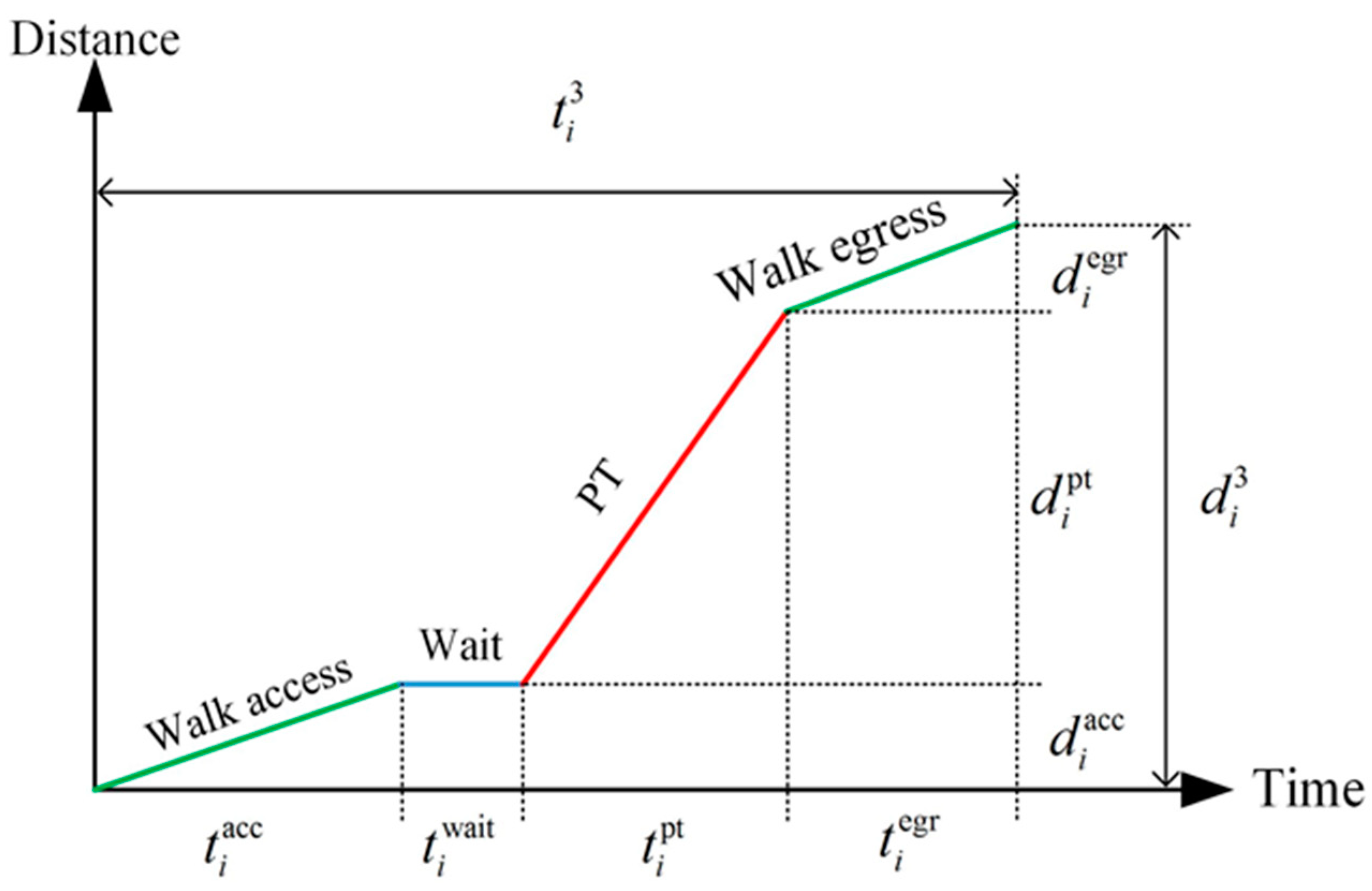
Figure 4 illustrates the modal-related 3-stage transit trip with walk access, one transit leg, and walk egress. Wait time at the platform is included in the trip. The walk access stage refers to the passengers’ walking distance from the trip origin to the transit platform. After passengers arrive at the platform, they wait for boarding before the in-vehicle stage. The walk egress stage includes the passengers’ walking distance from the transit platform to the trip destination.
As shown in Figure 4, transit trip i satisfies the following expressions on trip distance and duration:
d i 3 = d i acc + d i pt + d i egr
t i 3 = t i acc + t i wait + t i pt + t i egr
In Equation (1), d i acc , d i pt , d i egr and d i 3 are the surveyed distances. Among them, the stage distances of d i acc , d i pt , and d i egr have been derived from the declared information, such as the O/D locations and transit stops. It is worth noting that the related distances are Euclidian distances. In Equation (2), the trip time t i 3 is surveyed and other travel time components are unknown, which signifies that they need to be inferred. According to the physical kinematics, t i acc + t i egr and t i pt can be calculated by:
{ t i acc + t i egr = ( d i acc + d i egr ) u i + ε i ( 1 ) t i pt = d i pt v i + ε i ( 2 )
where u i adopts the average walking speed by age groups from reference [21], i.e., 4.3 km/h~4.8 km/h; v i is the average transit speed that needs to be inferred; ε i ( 1 ) and ε i ( 2 ) are error items. In this study, for railway transit modes, such as train and metro (except tramway), d i acc and d i egr are both updated by the sum of two parts: (1) the surveyed values (i.e., distance from origin to station entrance or from station exit to destination), and (2) the estimated mean distance c inside the station for the access or egress stage. Here, c is set to 250 m, according to the study in [22]. Thus, Equation (2) is updated by:
t i 3 d i acc + d i egr + 2 c u i = t i wait + d i pt v i + ε i
We assume that there exists a linear relationship between t 3 ( d acc + d egr + 2 c ) / u and d pt when the wait time t wait and transit speed v become constants. Thus, t wait and v can be estimated by the coefficients through the simple linear regression model y = β 0 + β 1 x + ε .
The passengers’ average wait time for public transport varies by different modes and time periods of the day. Regarding different land-use patterns and urbanization in the region, the average transit speeds should be different in the urban and rural areas, particularly for the bus speeds. Therefore, the trips are segmented by time periods and modes. In other words, d i pt , t i wait and v i in Equation (4) are associated with these two attributes. For wait time inferences, we set the indices of time periods p = 1 , , n and the indices of transit modes q = 1 , , m . For transit speed inferences, we set the indices of transit sub-modes r = 1 , , l . In our study, there is a total of four time periods (i.e., AM peak, inter peak, PM peak, and off peak) and three transit modes (i.e., train, metro, and bus), or four sub-modes (i.e., train, metro, bus_urb, and bus_sub) with the consideration of space.
Giving that y i = t i 3 ( d i acc + d i egr + 2 c ) / u i , we build the following linear regression model as:
y i = β 0 + β 1 , 1 ( 1 ) e i , 1 , 1 ( 1 ) + β 1 , 2 ( 1 ) e i , 1 , 2 ( 1 ) + + β n , m ( 1 ) e i , n , m ( 1 ) + β 1 ( 2 ) e i , 1 ( 2 ) d i , 1 pt + β 2 ( 2 ) e i , 2 ( 2 ) d i , 2 pt + + β l ( 2 ) e i , l ( 2 ) d i , l pt + ε i
where e i , p , q ( 1 ) and e i , r ( 2 ) are dummy values of 0 or 1. As a whole, there are n × m + l explanatory variables in Equation (5). Assuming that trip i with the time and mode attributes correspond to the indices of p, q and r, we then have e i , p , q ( 1 ) = 1 and e i , r ( 2 ) = 1 . According to Equations (4) and (5), we estimate the wait time and mode speed by:
t i , p , q wait = β 0 + β p , q ( 1 ) e i , p , q ( 1 ) = β 0 + β p , q ( 1 )
v i , r = 1 β r ( 2 ) e i , r ( 2 ) = 1 β r ( 2 )
The matrix notation for Equation (5) with k observations (i.e., i = 1, 2, …, k) can be written as:
y = X β   +   ε
where
y = ( y 1 , y 2 , , y k ) T X = ( 1 x 1 , 1 ( 1 ) x 1 , 2 ( 1 ) x n , m ( 1 ) x 1 ( 2 ) x 2 ( 2 ) x l ( 2 ) ) = ( 1 1 1 e 1 , 1 , 1 ( 1 ) e 1 , 1 , 2 ( 1 ) e 1 , n , m ( 1 ) e 2 , 1 , 1 ( 1 ) e 2 , 1 , 2 ( 1 ) e 2 , n , m ( 1 ) e k , 1 , 1 ( 1 ) e k , 1 , 2 ( 1 ) e k , n , m ( 1 ) e 1 , 1 ( 2 ) d 1 , 1 pt e 1 , 2 ( 2 ) d 1 , 2 pt e 1 , l ( 2 ) d 1 , l pt e 2 , 1 ( 2 ) d 2 , 1 pt e 2 , 2 ( 2 ) d 2 , 2 pt e 2 , l ( 2 ) d 2 , l pt e k , 1 ( 2 ) d k , 1 pt e k , 2 ( 2 ) d k , 2 pt e k , l ( 2 ) d k , l pt ) β = ( β 0 , β 1 , 1 ( 1 ) , β 1 , 2 ( 1 ) , , β n , m ( 1 ) , β 1 ( 2 ) , β 2 ( 2 ) , , β l ( 2 ) ) T ε = ( ε 1 , ε 2 , , ε k ) T
Generally, the above parameters in the vector of β can be estimated by the ordinary least squares (OLSs) method or the maximum likelihood estimation (MLE) method. The average wait time and transit speeds are finally obtained by:
t p , q wait = β 0 + β p , q ( 1 )
v r = 1 β r ( 2 )

3.3. Estimation of Transfer Time Based on 4-Stage Transit Trips

Due to a lack of time components information in the survey, the transfer time between two transit legs is defined by the total time of covering transfer distance, engaging in activities if applicable, and waiting for the transit mode. 
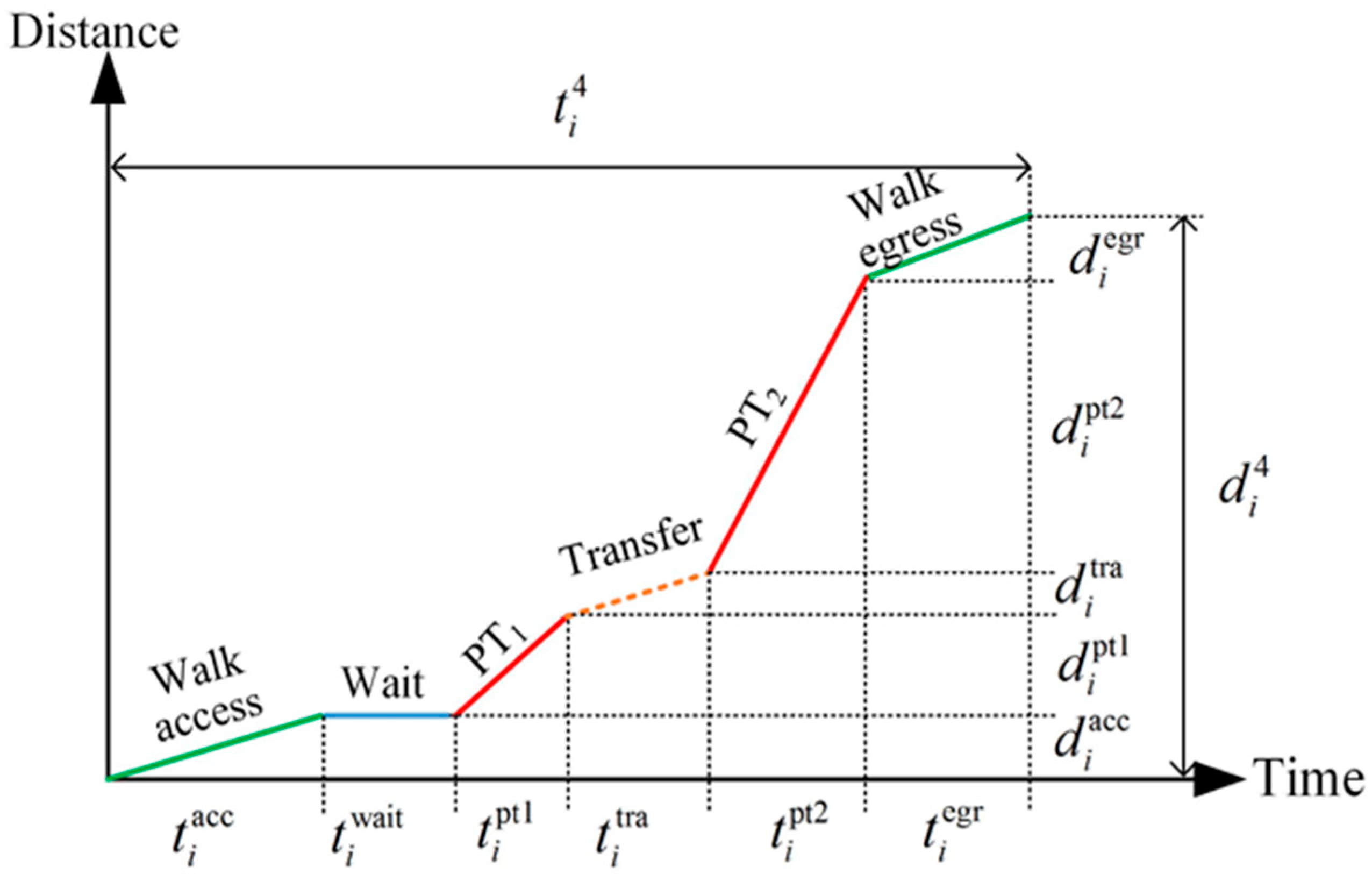
Figure 5 illustrates the modal-related 4-stage transit trips, including walk access and egress stages, and two PT stages. In addition, the wait time t i wait for the first PT stage and the transfer time t i tra for the second PT stage are included. The wait time is estimated from the previous 3-stage transit trips, and the transfer time needs to be inferred in this section.
Similar to the 3-stage transit trip in Figure 4, the 4-stage transit trip i satisfies Equations (11) and (12) in terms of travel distance and duration, respectively, and the values of d i acc , d i pt 1 , d i pt 2 , d i egr , d i 4 and t i 4 are known from the survey.
d i 4 = d i acc + d i pt 1 + d i tra + d i pt 2 + d i egr
t i 4 = t i acc + t i wait + t i pt 1 + t i tra + t i pt 2 + t i egr
From Equation (12), we have t i tra = t i 4 ( t i acc + t i egr ) t i wait t i pt 1 t i pt 2 . According to the inferences of average wait time and transit mode speeds (see Equations (6) and (7) in Section 3.2), the transfer time for each trip i is estimated by:
t i tra t ^ i tra = t i 4 ( d i acc + d i egr + 2 c ) u i t i , p , q wait d i pt 1 v i , r 1 d i pt 2 v i , r 2
where trip i has the attributes of time period p, the first waiting transit mode q, the transit sub-modes for the two PT stages r1 and r2, and t ^ i tra is the estimated transfer time, being subject to t ^ i tra > 0 . For the trips with attributes corresponding to p, q, r1, and r2, noted as p , q , r 1 , r 2 Z ( i ) , the average transfer time is calculated by:
t p , r 1 , r 2 tra = 1 N p , r 1 , r 2 Z ( i ) t ^ i tra

4. Results

4.1. Estimated Wait Time and Mode Speeds

The average wait time and transit speeds are calculated by Equations (9) and (10), according to the linear regression model based on the 3-stage transit trips. The “lm” package in the R toolbox is used to estimate the parameters of the model. The regression results are shown in Table 3.
We find that the coefficients of the linear model are significantly estimated. The coefficients that perform the worst are related to the bus mode’s wait time estimations (i.e., x 1 , 3 ( 1 ) , x 2 , 3 ( 1 ) , and x 3 , 3 ( 1 ) ), which still reach the confidence level of 90%. In theory, if two or more explanatory variables in a model have a perfect linear relationship, then not every regression coefficient in the model can be estimated due to the singularity. Using the correlation analysis method in [23], we find that x 4 , 3 ( 1 ) (variable assigned to bus in the off peak) is the linearly dependent term, and we thus remove it from the model. Through Equation (9), only the related wait time for the bus in the off peak is equivalent to β 0 , namely the coefficient associated with the intercept of the linear model. Other wait times for the time period p and the transit mode q are calculated by the sum of β 0 and the coefficient associated with the variable x p , q ( 1 ) . Through Equation (10), the speed of transit mode r is estimated by the reciprocal value of x r ( 2 ) . Table 4 summarizes the estimated average wait time and speeds for all transit modes. We find that passengers spent less waiting time at railway platforms during the AM peak, due to the higher service frequency. The same evidence can also be found in [3]. On the contrary, the longer waiting time at the PM peak may reflect the situation of passengers being left at platforms to wait for the next trains due to the limited train capacity and the high crowding levels at the platforms. It is reasonable that the average suburban bus speed is higher than the urban bus speed. Regarding the results’ reliability, we discuss it further in Section 5.
In Figure 6, we illustrate the linear regression model in a disaggregate way for the different transit modes and time periods. The red lines are the fitted linear models. The black dots are the observed values: y equals the sum of transit in-vehicle time and wait time (in min), and x is the travel distance (in km). As a whole, the illustration indicates the acceptable goodness-of-fit case by case, even though the related parameters are concurrently estimated from our integrated linear regression model, instead of the disaggregate ones that are based on their own data samples.

4.2. Transfer Time

4.2.1. Transfer Analysis in Time and Space

As mentioned in Section 3.3, the transfer time between two kinds of transit modes or lines is estimated using the transit trips of Modality 4, i.e., walk access—PT—PT—walk egress. Table 5 shows the transfer frequency matrix. Besides the train and metro, the sub-modes of urban bus and suburban bus are included. Most of the transfers happened between two metro lines (about 35%), followed by the transfers from metro to train, and then the transfers from train to metro. There are very few transfers between bus_urb and bus_sub.
According to Equation (14), we estimate the mean transfer time for each time period, as shown in Figure 7. For simplification, the modes of train, metro, bus_urb, and bus_sub are abbreviated by “T”, “M”, “BU”, and “BS”, respectively. As a whole, we find that the transfer from bus to railway (i.e., train or metro), especially from urban bus to metro, performs better than the transfer from railway to bus. As for the transfer to train, the suburban bus is more convenient than the urban bus. This makes sense because more centered transit hubs were built in the suburb. We also find that the transfers take a relatively long time between the urban buses or between the suburban buses, more than 15 min on average. For different time periods, passengers undergo less transfer time from the railway transit modes of train and metro to the urban bus at the inter-peak hours (about 12.6 min), compared to those during other periods (15~19 min). This may be explained by the crowding of passengers in the urban areas, leading to a less efficient transfer experience in the morning and evening peak hours. The lower transit service frequency at the off-peak hours will also cause more waiting time in a transfer. On the contrary, in suburbs, the transfer from the train to the bus takes more time in the inter peak (about 15.6 min), while it takes less time in the AM and PM peaks (about 13 min). It is worth noting that the blank parts without values are due to the lack of trip data.
Figure 8 shows spatially the transfer time to train, metro, and bus during the AM and PM peak hours. In Figure 8a, during the AM peak, the transfer time from any mode to the train is less than 20 min in the urban areas (i.e., Paris and the inner ring), and even less in some rural areas (less than 10 min). For the transfer to the metro in Paris, it takes less than 10 min. The transfer time to the bus almost refers to two levels: (1) 10 min to 20 min; (2) ≥20 min. Most of the transfers for buses of more than 20 min occurred in the inner ring. In Figure 8b, during the PM peak, the locations of transfers to train are centered in Paris and a small part of the transfers are located nearby. The metro transfer locations are clearly regrouped and some locations near the periphery require more time, i.e., 10 min–20 min. Most of the transfers to the bus of less 20 min are located in the eastern part of the inner ring, and some are expanded to the outer ring, compared to those in Figure 8a.

4.2.2. Validation

The validation process here is conducted by comparing two kinds of transfer time based on the 5-stage transit trips with three transit legs. The reference transfer time is calculated based on the transfer time estimated from the 4-stage transit trips (see Figure 7). We directly add up the two transfer times among the three transit stages as the reference. The compared transfer time is calculated by the rest of the travel time after subtracting the average walking time, wait time, and in-vehicle time (derived from the transit mode speeds), similar to Equations (13) and (14). As a result, we obtain all the pairs of transfer time for all the chains of three transit legs within the trips, as shown in Figure 9. The chains of BS→T→BU, BS→T→T, BU→BU→M, M→M→BU, M→M→M, M→M→T, T→BS→M, T→M→BS, and T→T→BU are well validated, in which only small gaps exist. As a whole, the average validation ratio (i.e., 100% minus the percentage of errors) for all the chains is 76.1%. This “inner” validation process also reflects the biases of transfer time in different transit trip patterns.

5. Discussion

At first, we discuss the data accuracy and the limitations of using the HTS for this study. Similar to other traditional and large-scale HTSs, there is no declared information about transfer time and in-vehicle time, only about the entire journey time from trip origin to destination. Our proposed method can estimate the transfer time after the decomposition of the journey time. Thus, precisely estimating the time components becomes the key issue. As sojourn locations (such as trip O/D, stage-based start/end locations) are easily declared in the survey, the travel distance per trip or stage is represented by the Euclidian distance between two recorded locations, instead of the route distance. These Euclidian distances are used for the estimation of time components at the stage level. The underestimated distances may cause the bias on time estimation. To reach the real experienced distance, the Euclidian distance can be weighted by adjusted factors, regarding different travel modes and GIS information. In the era of big data, it is possible to obtain the route distance, for example, using GPS tracking data from mobile phones [24].
In the interest of the method’s robustness, we used the integrated linear regression model with all considered explanatory variables, instead of the disaggregate linear regression model for each mode and time period. There are two reasons. First, the parameters associated with transit speeds are estimated by the integrated model with the assumption of time independence for mode speeds. This reduces the estimation errors caused by insufficient samples during the off-peak hours (see Figure 6). Second, the integrated model is more flexible in terms of aggregating the variables that are assumed to have no dependence on time and space, so as to reduce the number of variables and ease our analysis. Although the obtained results have statistical significance, they seem overestimated. For example, in the Paris region, it is reported that the average commercial speed of RER A (one train line in the region) is about 49 km/h, the metro speed is between 21 km/h and 27 km/h, and the speed of bus on priority lanes is about 12 km/h [25]. Our estimated railway transit speeds, which were estimated based on the Euclidian distance, are close to the aforementioned commercial speeds, but will be greater after the adjustment by factor over one when considering the route distance. This overestimation is more evident in the bus speed comparison. It may be caused by the sample representativeness (e.g., many short bus trips in the sample) and the declaration bias of travel time in the HTS. One possible solution may be using the weighted regression model to estimate appropriate parameters [26]. As the model fitting performance is still satisfied in our study, it has the potential for model extension in a more general case study. For any modes, as long as the modal distance traveled is known, the average mode speed can be estimated through the proposed linear regression model, and the time cost can consequently be calculated. This is also applicable to other more efficient access and egress modes compared to walking, such as bicycles, scooters, and shared vehicles.
As for practice, the obtained results have potential to guide transit operations in the study area. For example, bus frequency needs to be coordinated with the time frequency of railway systems, especially for the passengers’ transfers from trains to buses in the urban area (see Figure 7). In some areas where the transfer time for buses is more than 20 min during the peak hours (see Figure 8), this indicates the imperfect reliability of bus travel time. We may have two ways to improve it. First, bus stops and passageways can be designed coordinately to avoid many conflicts with high-density traffic flows. Second, we can establish bus-dedicated or priority lanes to ensure the bus arrives on time or deploy the transport hubs in locations that would allow for the transfer to become seamless. Moreover, the reduction of the transfer time in rural areas deserves a special concern from our study, and a more accurate time-dependent OD demand might be required for transit operations. The passenger security at peak hours should also be paid attention to. This is notably important for the large and complex transit system in the Paris region. A trade-off may exist between transfer time and ensuring passengers’ security.

6. Conclusions

This paper aims to estimate the transfer time in the multimodal transit networks from the most recent HTS in the Paris region. The average wait time and transit mode speeds are initially estimated by the linear regression model. The related inferences of transfer time in different time periods and space are investigated. From the study, some evidence is worth mentioning. In the Paris region, the transfer to the train or metro costs less time than the transfer to the bus. The transfers between the suburban buses cost a little more than the transfers between the urban buses. Regarding the different time periods, the inter peak period seems to be the best time for transfers from the railway system (both train and metro) to the bus. Our preliminary results are more qualitatively reliable than the estimated values themselves, which are subject to the sample size for the regression model, declaration bias in the HTS, and some ignored influential variables.
The current work could be extended by three aspects in the future. First, the dataset of the transit trips is anticipated to be enriched in application to the proposed model. Once the HTS is completely finished for the survey planning horizon, the study can be replicated and more representative results may be generated. Second, other kinds of datasets, such as GPS traces and automated fare collection data, will be considered to further validate and complement our estimated results. At last, the socio-economic relationship can be established in the model to find the preferences of targeted passenger groups in the transit system.

Author Contributions

Conceptualization, B.Y. and F.L.; methodology, B.Y. and F.L.; software, B.Y.; validation, B.Y. and F.L.; formal analysis, B.Y.; writing—original draft preparation, B.Y.; writing—review and editing, B.Y. and F.L.; visualization, B.Y.; supervision, F.L. All authors have read and agreed to the published version of the manuscript.

Funding

This research received no external funding.

Institutional Review Board Statement

Not applicable.

Informed Consent Statement

Not applicable.

Data Availability Statement

Data can be made available upon request for collaboration.

Acknowledgments

This work is supported by the ENPC-IDFM research chair on territorial mobility. We thank the regional mobility organizing authority—Île-de-France Mobilités (IDFM)—for providing us with the household travel survey data (i.e., EGT H2020) in their first survey stage of 2018–2019.

Conflicts of Interest

The authors declare no conflict of interest.

References

  1. Seaborn, C.; Attanucci, J.; Wilson, N.H.M. Analyzing multimodal public transport journeys in London with smart card fare payment data. Transp. Res. Rec. 2009, 2121, 55–62. [Google Scholar] [CrossRef]
  2. Kieu, L.M.; Bhaskar, A.; Chung, E. Public transport travel-time variability definitions and monitoring. J. Transp. Eng. 2015, 141, 04014068. [Google Scholar] [CrossRef] [Green Version]
  3. Sun, Y.; Xu, R. Rail transit travel time reliability and estimation of passenger route choice behavior. Transp. Res. Rec. 2012, 2275, 58–67. [Google Scholar] [CrossRef]
  4. Dixit, M.; Brands, T.; van Oort, N.; Cats, O.; Hoogendoorn, S. Passenger travel time reliability for multimodal public transport journeys. Transp. Res. Rec. 2019, 2673, 149–160. [Google Scholar] [CrossRef] [Green Version]
  5. Krygsman, S.; Dijst, M.; Arentze, T. Multimodal public transport: An analysis of travel time elements and the interconnectivity ratio. Transp. Policy 2004, 11, 265–275. [Google Scholar] [CrossRef]
  6. Eltved, M.; Lemaitre, P.; Petersen, N.C. Estimation of transfer walking time distribution in multimodal public transport systems based on smart card data. Transp. Res. Part C Emerg. Technol. 2021, 132, 103332. [Google Scholar] [CrossRef]
  7. Tavassoli, A.; Mesbah, M.; Shobeirinejad, A. Modelling passenger waiting time using large-scale automatic fare collection data: An Australian case study. Transp. Res. Part F Traffic Psychol. Behav. 2018, 58, 500–510. [Google Scholar] [CrossRef]
  8. Knoppers, P.; Muller, T. Optimized transfer opportunities in public transport. Transp. Sci. 1995, 29, 101–105. [Google Scholar] [CrossRef]
  9. Lee, A.; Van Oort, N.; Van Nes, R. Service reliability in a network context: Impacts of synchronizing schedules in long headway services. Transp. Res. Rec. 2014, 2417, 18–26. [Google Scholar] [CrossRef] [Green Version]
  10. Schakenbos, R.; Paix, L.L.; Nijenstein, S.; Geurs, K.T. Valuation of a transfer in a multimodal public transport trip. Transp. Policy 2016, 46, 72–81. [Google Scholar] [CrossRef]
  11. Wahaballa, A.M.; Kurauchi, F.; Schmöcker, J.-D.; Iwamoto, T. Rail-to-Bus and Bus-to-Rail transfer time distributions estimation based on passive data. In Proceedings of the 14th Conference on Advanced Systems in Public Transport and Transit Data 2018, Brisbane, Australien, 23–25 July 2018; pp. 1–7. [Google Scholar]
  12. Ma, Z.; Ferreira, L.; Mesbah, M.; Zhu, S. Modeling distributions of travel time variability for bus operations. J. Adv. Transp. 2016, 50, 6–24. [Google Scholar] [CrossRef]
  13. Mazloumi, E.; Currie, G.; Rose, G. Using GPS data to gain insight into public transport travel time variability. J. Transp. Eng. 2010, 136, 623–631. [Google Scholar] [CrossRef]
  14. Singh, R.; Hörcher, D.; Graham, D.J.; Anderson, R.J. Decomposing journey times on urban metro systems via semiparametric mixed methods. Transp. Res. Part C Emerg. Technol. 2020, 114, 140–163. [Google Scholar] [CrossRef]
  15. Ma, X.; Wu, Y.J.; Wang, Y.; Chen, F.; Liu, J. Mining smart card data for transit riders’ travel patterns. Transp. Res. Part C Emerg. Technol. 2013, 36, 1–12. [Google Scholar] [CrossRef]
  16. Wahaballa, A.M.; Kurauchi, F.; Yamamoto, T.; Schmöcker, J.D. Estimation of platform waiting time distribution considering service reliability based on smart card data and performance reports. Transp. Res. Rec. 2017, 2652, 30–38. [Google Scholar] [CrossRef]
  17. INSEE Population Légale de l’Île-de-France in 2020. Available online: https://www.insee.fr/fr/statistiques/5351310 (accessed on 9 July 2021).
  18. Île-de-France Mobilités; OMNIL. DRIEA Enquête Globale Transport (EGT) H2020–Résultats Partiels. 2018. Available online: http://www.omnil.fr/spip.php?article229 (accessed on 10 November 2020).
  19. Yin, B.; Leurent, F. What are the multimodal patterns of individual mobility at the day level in the Paris region? A two-stage data-driven approach based on the 2018 Household Travel Survey. Transportation 2022. [Google Scholar] [CrossRef]
  20. DRIEA-IDF Modélisation des Déplacements en IDF avec MODUS 3.1. Available online: https://www.drieat.ile-de-france.developpement-durable.gouv.fr/IMG/pdf/modelisation_des_deplacements_en_idf_avec_modus_3.1.pdf (accessed on 1 October 2022).
  21. Schimpl, M.; Moore, C.; Lederer, C.; Neuhaus, A.; Sambrook, J.; Danesh, J.; Ouwehand, W.; Daumer, M. Association between walking speed and age in healthy, free-living individuals using mobile accelerometry-a cross-sectional study. PLoS ONE 2011, 6, e23299. [Google Scholar] [CrossRef] [PubMed]
  22. Leurent, F.; Xie, X. On individual repositioning distance along platform during train waiting. J. Adv. Transp. 2018, 2018, 4264528. [Google Scholar] [CrossRef]
  23. Chambers, J.M.; Freeny, A.E.; Heiberger, R.M. Analysis of Variance; Designed Experiments. In Statistical Models in S; Routledge: New York, NY, USA, 2018; pp. 145–193. [Google Scholar] [CrossRef]
  24. Yin, B.; Leurent, F. Exploring individual activity-travel patterns based on geolocation data from mobile phones. Transp. Res. Rec. 2021, 2675, 771–783. [Google Scholar] [CrossRef]
  25. Île-de-France Le Grand Paris des Transports. Available online: https://www.prefectures-regions.gouv.fr/ile-de-france/Region-et-institutions/Portrait-de-la-region/Le-Grand-Paris/Le-Grand-Paris-des-transports/Le-Grand-Paris-des-transports#:~:text=Cette%20vitesse%20est%20%C3%A9galement%20sans,disposent%20d%E2%80%99un%20couloir%20prioritaire (accessed on 5 October 2022).
  26. Ma, X.; Zhang, J.; Ding, C.; Wang, Y. A geographically and temporally weighted regression model to explore the spatiotemporal influence of built environment on transit ridership. Comput. Environ. Urban Syst. 2018, 70, 113–124. [Google Scholar] [CrossRef]
Figure 1. Distribution of railway stations and lines.
Futuretransp 02 00049 g001
Figure 2. Distribution of walk distance in access and egress stages.
Futuretransp 02 00049 g002
Figure 3. Transit trip (with modalities 3, 4, and 5) volumes in different time periods.
Futuretransp 02 00049 g003
Figure 4. Diagram of 3-stage transit trip: Walk access—PT—Walk egress.
Futuretransp 02 00049 g004
Figure 5. Diagram of 4-stage transit trip: Walk access—PT1—PT2–Walk egress.
Futuretransp 02 00049 g005
Figure 6. Fitting results of the linear regression model.
Futuretransp 02 00049 g006
Figure 7. Average transfer time in the Paris region.
Futuretransp 02 00049 g007
Figure 8. Geographical distribution of transfer time during: (a) AM peak; (b) PM peak.
Futuretransp 02 00049 g008
Figure 9. Comparison of transfer time inferred from the two kinds of trips.
Futuretransp 02 00049 g009
Table 1. Overview of population and territory in Île-de-France (Source: INSEE 2020).
Urbanization Scale
(Department)
Paris
(75)
Inner Ring
(92,93,94)
Outer Ring
(77,78,91,95)
Population (×106)2.14.75.5
Jobs (×106)1.81.52.6
Surface (km2)10565711,250
Table 2. Trip splits by the number of stages per trip.
No. of Stages Per Trip12345≥6
Trip percentage (%)63.110.915.87.02.60.6
Table 3. Results of the linear regression model.
Variables (X)Coefficients (β)Std. Errort ValuesP(>|t|)
Intercept18.032.108.580.00
x 1 , 1 ( 1 ) −10.232.57−3.970.00
x 1 , 2 ( 1 ) −15.392.42−6.370.00
x 1 , 3 ( 1 ) −3.242.04−1.590.11
x 2 , 1 ( 1 ) −9.212.57−3.590.00
x 2 , 2 ( 1 ) −13.702.37−5.780.00
x 2 , 3 ( 1 ) −3.082.02−1.530.13
x 3 , 1 ( 1 ) −7.672.51−3.060.00
x 3 , 2 ( 1 ) −12.642.34−5.400.00
x 3 , 3 ( 1 ) −3.482.01−1.730.08
x 4 , 1 ( 1 ) −7.803.27−2.390.02
x 4 , 2 ( 1 ) −11.472.55−4.490.00
x 1 ( 2 ) 1.240.1012.240.00
x 2 ( 2 ) 2.530.2410.720.00
x 3 ( 2 ) 3.460.3210.800.00
x 4 ( 2 ) 2.790.328.810.00
R2:0.3524
Observations:1304
Table 4. Estimation of average wait time and speeds of transit modes.
TrainMetroBus
Wait time (min)AM peak7.82.614.8
Inter peak8.84.314.9
PM peak10.45.414.5
Off peak10.26.618.0
Transit speeds (km/h)48.323.717.4 (urban), 21.5 (suburb)
Table 5. Transfer frequency between two transit modes.
ToTrainMetroBus_urbBus_sub
FromTrain120 (11%)140 (13%)53 (5%)39 (4%)
Metro151 (14%)376 (35%)22 (2%)5 (0%)
Bus_urb41 (4%)15 (1%)44 (4%)0 (0%)
Bus_sub35 (3 %)3 (0%)2 (0%)27 (3%)
Publisher’s Note: MDPI stays neutral with regard to jurisdictional claims in published maps and institutional affiliations.

