Article

Crash Patterns in the COVID-19 Pandemic: The Tale of Four Florida Counties

by
Mohammadreza Koloushani
1,
Mahyar Ghorbanzadeh
1,
Eren Erman Ozguven
1,* and
Mehmet Baran Ulak
2
1
Department of Civil and Environmental Engineering, FAMU–FSU College of Engineering, Tallahassee, FL 32310, USA
2
Department of Civil Engineering, University of Twente, 7522 NB Enschede, The Netherlands
*
Author to whom correspondence should be addressed.
Future Transp. 2021, 1(3), 414-442; https://doi.org/10.3390/futuretransp1030023
Submission received: 21 August 2021 / Revised: 9 September 2021 / Accepted: 9 September 2021 / Published: 24 September 2021

Abstract

:
This study investigates the impacts of the noticeable change in mobility during the COVID-19 pandemic with analyzing its impact on the spatiotemporal patterns of crashes in four demographically different counties in Florida. We employed three methods: (1) a Geographic Information System (GIS)-based method to visualize the spatial differences in crash density patterns, (2) a non-parametric method (Kruskal–Wallis) to examine whether the changes in crash densities are statistically significant, and (3) a negative binomial regression-based approach to identify the significant socio-demographic and transportation-related factors contributing to crash count decrease during COVID-19. Results confirm significant differences in crash densities during the pandemic. This may be due to maintaining social distancing protocols and curfew imposement in all four counties regardless of their sociodemographic dissimilarities. Negative binomial regression results reveal that the presence of youth populations in Leon County are highly correlated with the crash count decrease during COVID-19. Moreover, less crash count decrease in Hillsborough County U.S. Census blocks, mostly populated by the elderly, indicate that this certain age group maintained their mobility patterns, even during the pandemic. Findings have the potential to provide critical insights in dealing with safety concerns of the above-mentioned shifts in mobility patterns for demographically different areas.

1. Introduction

On 5 April 2021, the World Health Organization (WHO) announced that there were approximately 131 million confirmed COVID-19 cases all over the world [1]. The U.S., with more than 30 million COVID-19 cases and 554,064 total deaths, ranked first in the globe. Among the U.S. states, Florida ranked third after California and Texas in terms of the highest number of cases [2]. The Florida Department of Health announced 2,085,306 cases and 33,710 deaths due to coronavirus throughout the state, as of 5 April 2021 [3]. This issue becomes even more challenging when aging populations are considered, due to their cognitive, behavioral, and health limitations [4]. According to the Centers for Disease Control and Prevention (CDC), the older population (65+) and those with serious medical conditions such as lung disease, diabetes, and liver disease are at a higher risk of COVID-19 infection [2,5]. This is especially a serious issue in Florida, since more than 20% of the total population in the state are 65 years and older [6]. The expected growth among aging Floridians justifies a need to study the impact of the COVID-19 pandemic on mobility in the State of Florida, given its unique demographic characteristics and associated risks for the roadway users. In addition to the older population’s (65+) special needs and vulnerability to severe crashes, many researchers have recognized the need to study the severity and frequency of youth-involved roadway crashes and the relevant behavioral factors. For example, young drivers (aged 16 to 25) were found to be at greater risk of being involved in a crash that led to casualties compared with other age groups, and this greater danger was usually related to their propensity to take risks while driving [7] and lacking enough experience to handle critical adverse conditions while driving in various type of crashes [8]. Although most of the existing research has focused on the noticeable changes in mobility pattern during COVID-19 to limit person-to-person interaction, several important concerns remain unaddressed. In this study, we utilize the existing crash data during the COVID-19 pandemic to answer the following questions:
(1)
How, and to what extent, did the COVID-19-induced decrease in traffic flow impact the pattern of the crash density?
(2)
Were there any significant crash pattern differences in selected demographically different Florida counties during the pandemic?
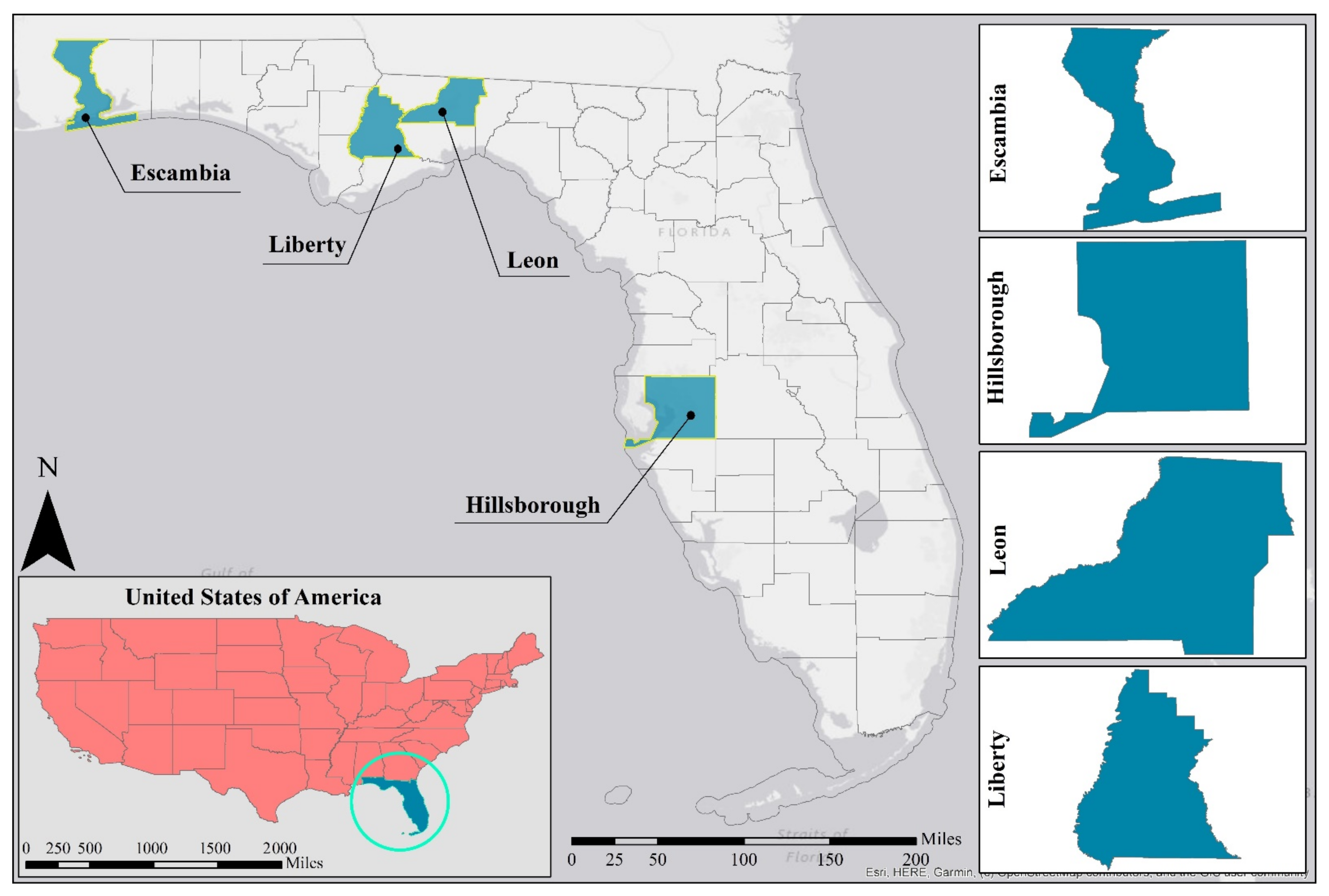
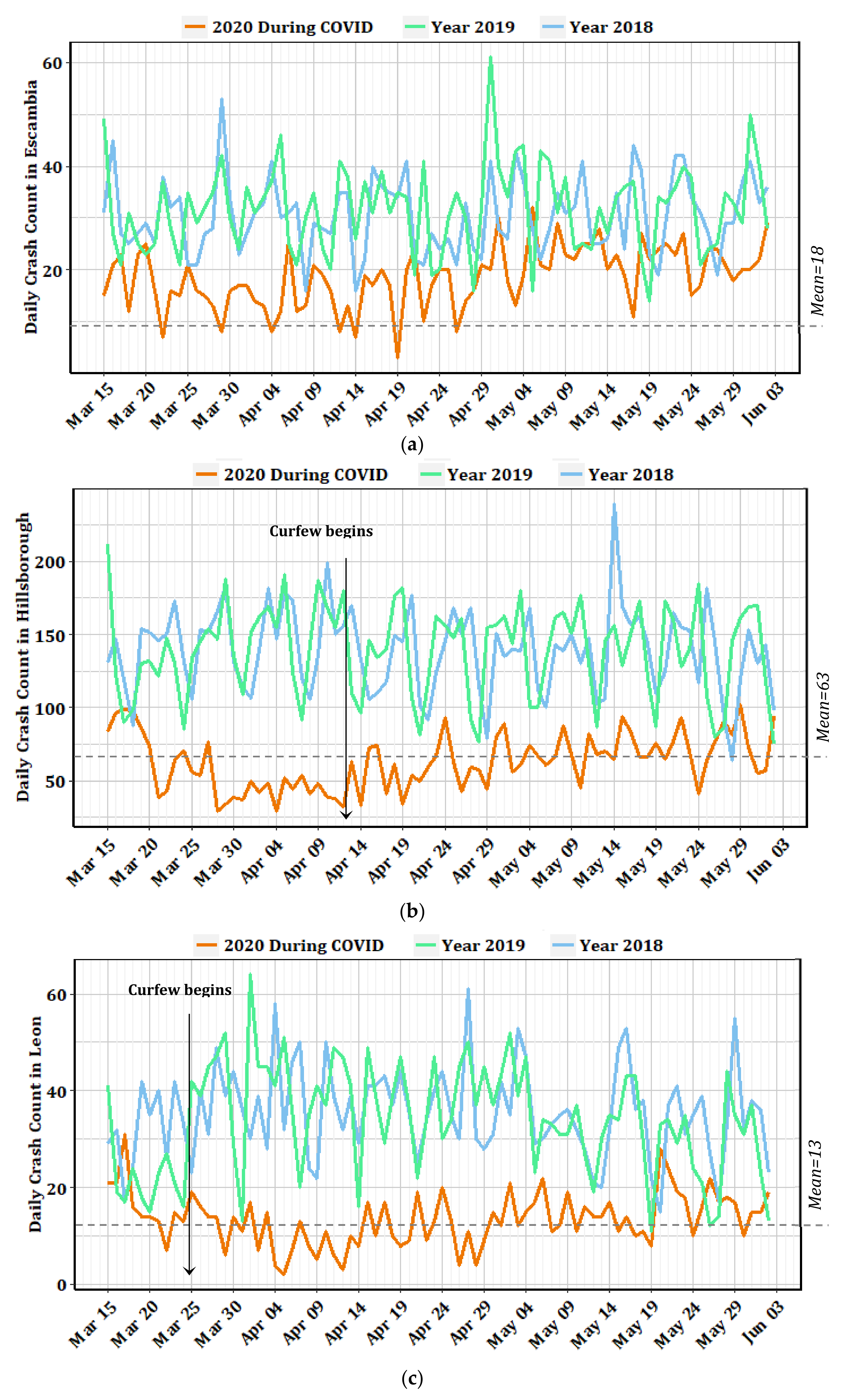
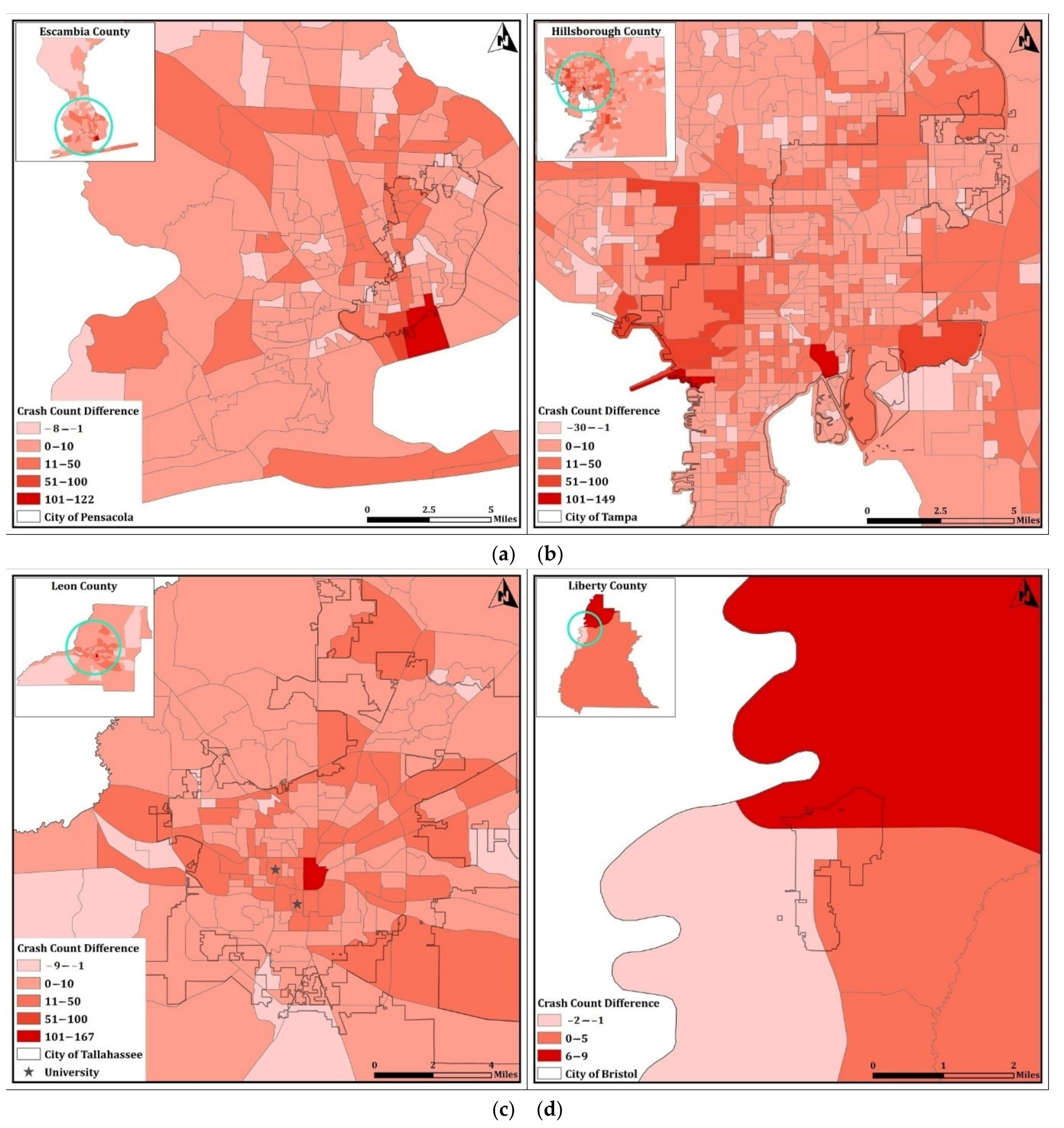
As such, with an extensive suite of spatial and statistical models, this research examines the impacts of the COVID-19 pandemic on the crash density patterns in four Florida counties; namely, Escambia (a mid-size county), Hillsborough (a metropolitan county), Leon (a mid-size college-oriented county which includes the state capital), and Liberty (a rural county) between 15 March 2020 and 2 June 2020 (we name this time period as “2020 After COVID”). Note that these counties have been selected due to their distinct demographic differences. We compare these patterns with those associated with three different periods: (a) 26 December 2019 and 14 March 2020 (2020 Before COVID), (b) the same period in 2019, and (c) the same period in 2018. To the authors’ knowledge, this type of comparative work has not been done previously. As a potential application, the findings of this study can assist state and local agencies in strategic planning efforts for coping with unpredictable COVID-19 impacts on mobility patterns, to improve safety and enhance mobility for road users from different age groups with certain characteristics. This type of analysis can help planners and emergency officials distinguish more vulnerable age groups and impose more efficient countermeasures during the COVID-19 pandemic for targeted populations.

2. Literature Review

There is a vast amount of literature focusing on mobility and crashes; however, this paper specifically focuses on those works that study COVID-19-related traffic safety and operations studies. For more information on the crash literature, please refer to: [9,10,11,12,13]. Specifically, GIS-based crash clustering has been utilized by many agencies to identify roadway segments and intersections that pose a high crash risk [14,15,16]. There are several clustering methods found in the literature, including Getis-Ord (Gi*) statistics [17,18], Bayesian spatiotemporal modeling [19], k-nearest neighbor (KNN) algorithm [20,21], kernel density estimation (KDE) [22], spatial weights matrices [23]. One of the common methodologies used for such a spatial analysis is kernel density estimation (KDE) which can identify the density of events. KDE is also adopted by this study to calculate the density differences between each pair of datasets, given the frequent and successful utilization of this method by previous studies [24,25,26].
Recent studies investigate the COVID-19 pandemic impacts on transportation from various aspects, including spatiotemporal of migration pattern during restrictions induced by the COVID-19 pandemic [27], accessibility to healthcare facilities [28,29], and traffic crashes and operations. According to Road Ecology Center at the University of California-Davis, the number of traffic crashes, crash-related injuries, and deaths were reduced by half during the first three weeks of the shelter-in-place order issued in California. Moreover, they reported a 55% reduction in the number of vehicles on California’s highways and a saving of USD 40 million per day [30,31]. Similarly, a 60% decline in traffic crashes, a 43% decline in deaths, and a 64% decline in injuries were observed due to the COVID-19 curfew in Turkey [32]. Brodeur et al. (2020) also found a 50% reduction in traffic collisions and USD 7 billion to USD 24 billion savings due to avoided car collisions after a stay-at-home order was issued in the states of Alabama, Connecticut, Kentucky, Missouri, and Vermont [33]. Moreover, Alabama Law Enforcement Agency stated a 48% decline in crashes in April 2020 compared to April 2019 [34]. The Alabama Department of Transportation also reported a 50% decrease in traffic volumes from 5 April 2020 to 23 April 2020, compared to the same period of the previous year [34]. Furthermore, the North Carolina Department of Transportation reported a drastic decline in the number of total crashes after the pandemic compared to the same period of 2019 in both urban and rural areas [35].
Moreover, National Police Foundation statistics showed a drastic decrease in the total number of total crashes in Florida, Iowa, Ohio, Massachusetts, and Missouri during the COVID-19 pandemic, specifically in March and April 2020. However, the findings indicated an increase in the fatality rates compared to the same period in 2019. They suggested that reduced traffic congestion would lead to higher speeds and reckless driving on the roads [36]. Similarly, the Indianapolis Star newspaper reported an average of 39% decrease in the traffic in Indianapolis, Indiana, from 2 March to 30 March 2020. Moreover, the number of crashes across the state dropped from 15,800 in March 2019 to 11,200 crashes in March 2020 [37]. Parr et al. [38] investigated the traffic volume patterns on urban and rural roadways across Florida during the COVID-19 pandemic in March 2020 and compared them with similar dates in 2019. Their findings indicated that the traffic volumes were reduced by 47.5% statewide. Furthermore, they found that the traffic decline in South Florida was less than in other areas in the state and people in southern parts of the state traveled more, although they were at a higher risk due to the more concentration of COVID-19 cases. They did not, however, investigate how, and to what extent, this drastic change in traffic volume patterns during the pandemic impact crash occurrences.
COVID-19 global pandemic has also significantly changed human mobility and travel patterns [39], resulting in a reduction in vehicle miles travel [40] and daily travel time [41]. Information technology-based activities (e.g., telecommuting, telemedicine, telehealth, telelearning) have been offering safer alternatives to physical traveling during the pandemic [42]. An analysis of traffic patterns during this period has identified that reduction in VMT has a significant negative relationship with COVID-19 cases and deaths across the USA [43]. This shows that people tend to avoid unnecessary travel and reduce social interactions that would occur during transportation [44]. Indeed, Doucette et al. (2021) showed that the mean daily VMT was reduced by 43% during the COVID-19 pandemic. Results also reveal that this decrease in VMT also led to less crashes, regardless of the level of injury [45]. Some researchers focused on safety performance functions (SPF), which demonstrated a positive correlation between AADT and crash counts [46,47].
The issue of reduced vehicle usage and ownership and its corresponding impact on various aspects of sustainable development (e.g., air pollution, economics, and traffic operations) have also been widely explored in the literature [48,49,50]. Zero emission policies have also encouraged many people to actively contribute to decreasing private vehicle usage through promoting alternative modes of transportation (i.e., public transit and biking) [51]. The COVID-19 pandemic may fade away soon or later; however, there is a potential that its impact on people’s tendency toward staying at home, working remotely, and lower private vehicle usage could last for a long time [52]. This will result in reduced vehicle usage and there is a need to investigate how demographically different areas would respond to this in terms of traffic operations and safety.
On the contrary to existing work, this study intends to investigate crash density reduction patterns in areas with different demographic characteristics. From this perspective, Florida is a particularly interesting case study to assess the traffic safety impacts of the COVID-19 due to (a) a high number of traffic crashes (i.e., Florida is among the top three states in the U.S.), (b) a high number of COVID-19 cases, and (c) a significant percentage of the senior population living in the state [38].
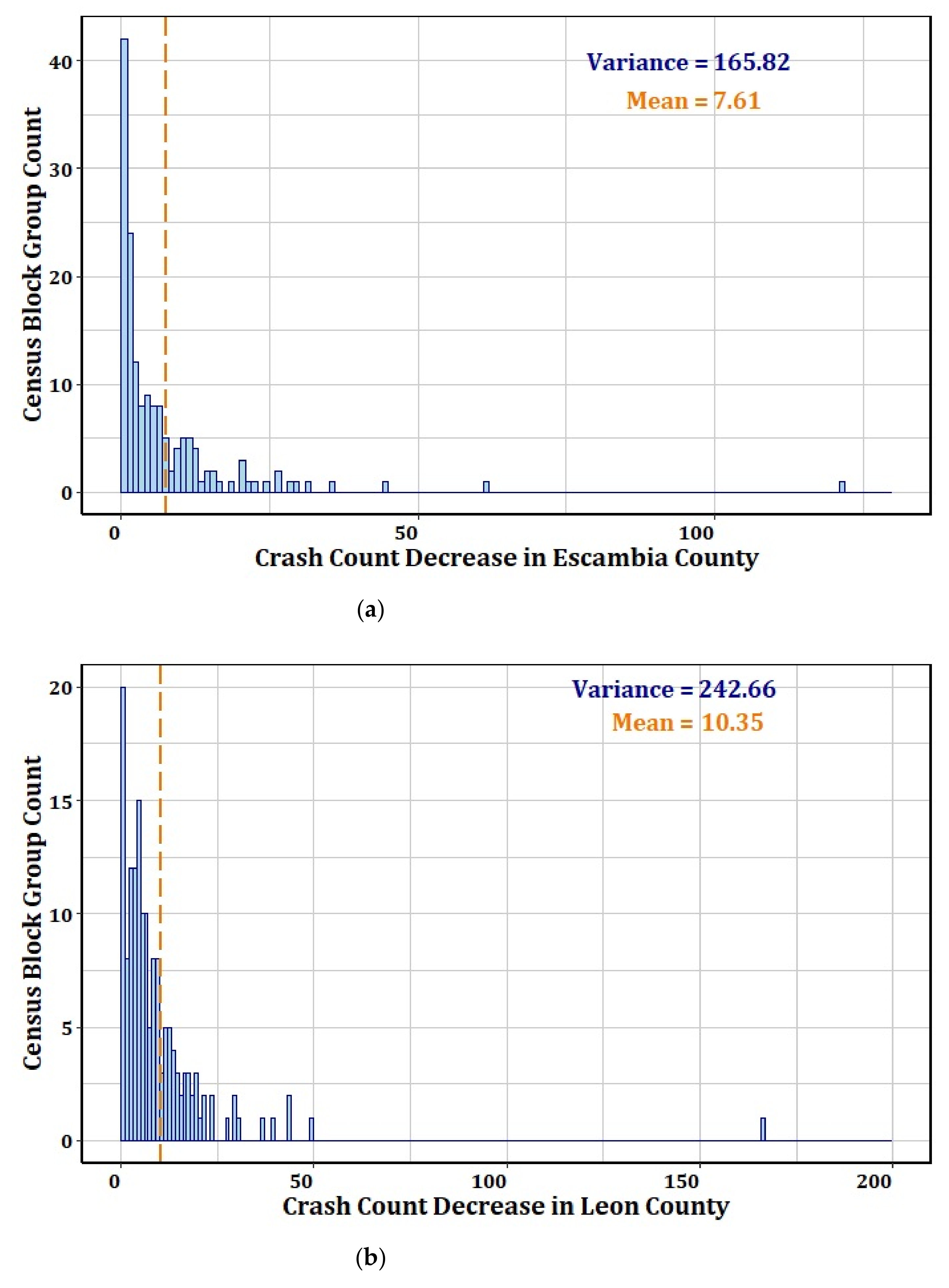
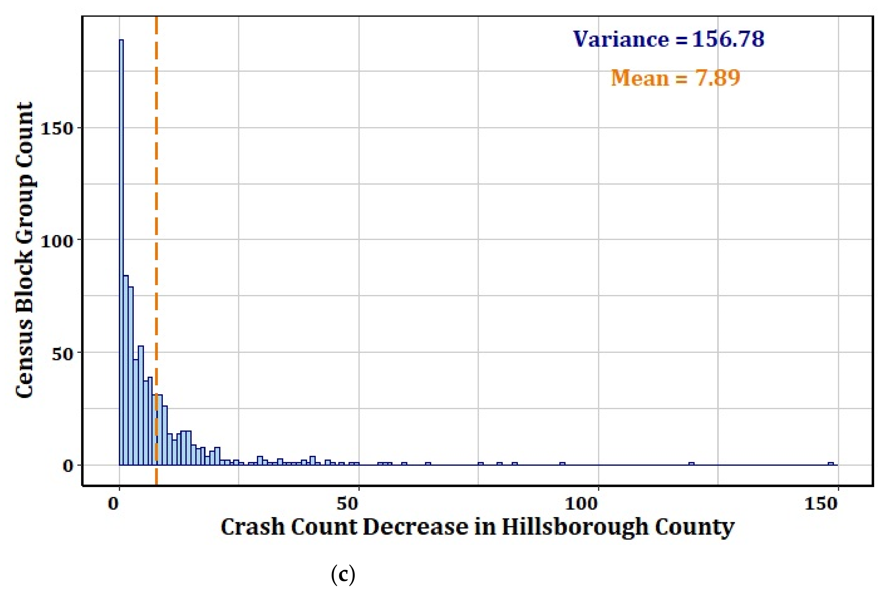
The remainder of the paper is as follows. First, the required crash data are described, followed by a brief review of the developed GIS-based methodology. The Kruskal–Wallis test results obtained from the differences of crash density are also provided to indicate whether these differences are statistically different or not. The KDE results for each county are, then, presented as separate maps for each time pair to indicate the pattern of crash density from a county-wide perspective. The sets of time series are also provided to (a) depict the temporal distribution of the total number of crashes that occurred during the COVID-19 pandemic, and (b) make a comparison possible for the same number of days in 2019, 2018, and 2020 before the COVID-19 pandemic. Moreover, an index is defined to compare crash patterns between different years to confirm that the crash density difference in 2020 was mainly due to the COVID-19 pandemic, not any other factors, including safety improvement measurements. Furthermore, three separate negative binomial regression (NBR) models were developed to statistically investigate the contribution of socio-demographic and transportation-related parameters on the crash count decrease (CCD) during the COVID-19 pandemic. Finally, the paper concludes with a summary, limitations, and recommendations for future research.

3. Study Area and Data Description

In this study, four counties of Florida were selected: Escambia (a mid-size county), Hillsborough (a metropolitan county), Leon (a college-oriented county that includes the state capital), and Liberty (a rural county). The illustration of the study area is presented in Figure 1. We selected these counties due to their distinct population characteristics which can help examine the effects of demographics on the spatial patterns of the crash densities [53]. Table 1 summarizes the statistical characteristics for each county, including demographic characteristics, transportation-related factors, college/university enrollment, and curfew policy details.

3.1. Demographic Data and Curfew Information

According to the 2014–2018 American Community Survey (ACS) estimates, as of 2018, Hillsborough County is the fourth populated county in Florida. Therefore, this research considered this metropolitan county to have distinguishing demographic features compared to the other counties (See Table 1). Escambia and Leon County, on the other hand, are considered mid-size counties based on their population. As shown in Table 1, Leon County has the highest average percentage of the youth (18–29) population (29.8%) in census block groups among all the other counties. Table 1 also illustrates that 23% of the total population in Leon County are enrolled in junior colleges, colleges, universities, and professional schools. Therefore, it is possible to consider this county as college-oriented, with a significant annual enrollment of 64,891. Escambia County, on the other hand, has the highest average percentage of aging (65+) population (17.3%) compared to Hillsborough and Leon County. This research also considers Liberty County, a rural county with just 6 census block groups, located in northwest Florida. Liberty County, with a population density of less than 100 persons per square mile, is delineated as a rural area based on definitions provided by ACS. This county has the lowest number of the population among the 67 counties in the state (8365). These demographic differences may result in different crash patterns caused by COVID-19; thus, we intend to assess this assumption in this paper.
In order to assess the impact of the curfew declarations during COVID-19, the dates when authorities imposed these curfews were also identified. Table 1 provides details regarding curfew orders in the last row. Note that no curfews were imposed in Escambia and Liberty counties. However, Florida Governor Ron DeSantis declared a state of emergency on 9 March 2020, announcing the closure of schools on 13 March. By 17 March, the governor closed all bars and nightclubs, and on 20 March, all restaurants were closed for dine-in service.

3.2. Crash Data

Based on previous research, we assumed that the variation in mobility patterns during the COVID-19 pandemic might impact the crash patterns, regardless of vehicle type and manner of collision [30,31,32,33,34,35]. As such, we considered all types of crashes and extracted crash data from the Signal Four Analytics website maintained by the University of Florida [54]. This 80-day data includes those crashes that occurred between 15 March 2020 through 2 June 2020, and the same periods in 2018 and 2019. In order to prepare a dataset containing crashes that occurred during a certain time to conduct a before-after study, there was a need to focus on a sample study period that clearly demonstrated the crash count decrease caused by COVID-19. For this purpose, the current research considered 15 March 2020 as the date when the total number of infected people (active cases) reached more than 100 cases for the first time. On this date, city authorities gradually started to impose some restrictions (e.g., curfew, lockdown, and social distancing measurements) to remedy this pandemic. Moreover, the crash data for the same number of days before the period of the COVID-19 pandemic (80 days between 26 December 2019 and 14 March 2020) were also acquired [54].
Table 2 shows the number of crashes and the mean values of AADT (average annual daily traffic) in each county, where we see noticeable decreases in the number of crashes in all counties during COVID-19. The most significant decrease (60%) is associated with Leon County, the one that has some distinguishing characteristics due to its college-oriented feature. As expected, most of the youth population that reside in this county have left, since the universities, colleges, and other educational centers were temporarily closed during the COVID-19. In addition, the decreases in the total number of crashes resulted from the COVID-19 pandemic compared to 2018 and 2019 follow the same trend in all four counties. Moreover, Table 2 also indicates that the mean values for AADTs in 2019 were greater than AADTs in 2020.
Moreover, we calculated the crash count decreases (CCD) at urban U.S. census block groups to estimate the effects of the socio-demographic and transportation-related independent variables on CCD. This was done for both studied 2019 and 2020 time periods (starting right when the COVID-19 pandemic did in 2020). Figure 2 shows that the distributions of CCDs violate the assumption of Poisson regression (i.e., unconditional means of the responses (CCDs) are smaller than their variances); therefore, negative binomial regression was utilized in this study, which has an extra parameter to model this over-dispersion [9].
It is also worth mentioning that the current research focused on urban census block groups and disregarded the ones that were located in rural areas. The rural census block groups have experienced a minor increase in the number of crashes during the pandemic; however, the range of increase is noticeably lower compared to urban areas and therefore these changes are negligible (see Figure 8 and Table 5). This issue has been discussed in detail in the “Results and Discussions” section.

4. Methodology

4.1. Spatial Analysis to Estimate Crash Densities

To examine the changes in crash density patterns stemming from the COVID-19 pandemic, we developed a Geographic Information Systems (GIS)-based methodology at the county level [55]. For this purpose, we used a kernel density estimation (KDE)-based clustering approach to examine the differences between spatial distributions of crash density pattern during the COVID-19 pandemic, and the other three crash datasets of three selected time periods with the same number of days. We realize that the KDE method is very sensitive to variation in its bandwidth parameter. This is because small bandwidths might discard the critical clusters by diminishing connections between points, whereas very large bandwidths might fail to identify local clusters by averaging out the effect of closely connected points. Hence, bandwidths were selected based on trial and error for each county [56,57].

4.2. Crash Density Comparison and Statistical Testing

Following the spatial analysis, a comparative crash density index was defined to identify the variation in crash density patterns resulting from the COVID-19 pandemic. The density difference (DD) approach was first proposed and utilized by Ulak et al. (2016) and adopted by Ghorbanzadeh et al. (2020) [58,59,60]. The formula of DD is shown in Equation (1):
D D i , j = D i D j
where D D i , j the density difference between the compared maps i and j, whereas D i and D j are the crash density values of the compared maps, respectively. We applied this measure for different time period crash density values as follows:
D D 2020   B e f o r e   C O V I D , 2020   A f t e r   C O V I D = D 2020   B e f o r e   C O V I D D 2020   A f t e r   C O V I D
D D 2019 , 2020   A f t e r   C O V I D = D 2019 D 2020   A f t e r   C O V I D
D D 2018 , 2020   A f t e r   C O V I D = D 2018 D 2020   A f t e r   C O V I D
Using three separate pairs of comparisons for each time period, we investigated the crash density differences in each county and assessed the assumption that the density difference does not follow the same pattern in counties that have various demographic characteristics. We also defined the fourth pair of comparisons between the same period of time in 2019 and 2018, in order to show that the variation in crash densities mainly resulted from the COVID-19 pandemic, not any other factors related to the safety improvement of infrastructure or other specific policies implemented to improve traffic safety.
D D 2019 , 2018 = D 2019 D 2018
Non-parametric methods have been widely used in literature, particularly in crash-related studies [61,62,63]. Distributions of all four datasets were not sufficiently normal based on skewness and kurtosis values. Thus, a non-parametric method, named Kruskal–Wallis one-way ANOVA, was employed to compare the density differences and determine if there are statistically significant differences between the crash density patterns.
In this research, we measured the pixel values in raster files corresponding with crash densities estimated by the KDE method for each period of time, during and before the COVID-19 pandemic. The Kruskal–Wallis method was performed to test the following hypothesis: There is a significant difference between crash densities due to COVID-19 and each one of the other datasets corresponding to time periods before COVID-19. This statistical method compares the means of two independent datasets to determine if there is a significant difference between each pair.

4.3. Modeling of the Reduction in Crash Counts

Crash counts are non-negative integer values by nature; hence, methods such as Poisson regression, negative binomial, and zero-inflated models are the most suited approaches to model crash counts [10,64]. Among these models, negative binomial regression (NBR) has been popular due to the overdispersion (the variance larger than the mean) problem that commonly occurs in crash data [65]. In this study, NBR models were developed to investigate the relationships between different demographics, socioeconomics, and transportation-related variables and crash count decrease (CCD) due to the COVID-19 pandemic. Before developing the NBR models, it was necessary to assign the total number of crashes to each census block group and calculate CCDs associated with them.
To deal with the assignment of crashes that occurred at the census block boundaries, this study proposed a proportional method that allocates these crashes to surrounding zones in proportion to the number of crashes (CC), which occurred completely inside the neighboring zones. The formula of CC is shown in Equation (2):
C C i = C C I i + j J i C C B i j C C I i C C I i + C C I j
where C C i is the total number of crashes assigned to the census block group, which is the sum of crashes that occurred completely within this census block group, represented by C C I i and the scaled crashes occurred at the shared boundaries ( C C B i j ), based on the proportion of inside crashes in the pairs of neighboring census block groups. In Equation (2), i indexes the census block groups and J i is the set of blocks located in the surrounding of census block i and having shared boundaries with it.
Using the total crash counts at each census block group, Poisson regression models were developed and the quotient of residual deviance and degree of freedom were calculated in order to verify the need for NBR. Since these quotients were identified to be greater than one, the NBR models were considered [66].
A subset of predictor variables has been considered to develop NBR models for each county, based on the Pearson correlation coefficients, forward selection method, literature review, and authors’ prior knowledge. The dependent variable, crash count decrease—CCD—was formulized as shown in Equation (3):
C C D i = C C i , 2019 C C i , C O V I D
where C C D i is the crash count decrease in census block group i, C C i , 2019 and C C i , C O V I D are the crash counts in ith census block during 2019 and the COVID-19 pandemic, respectively. C C D i is a count variable that can only take non-negative integer values and the expectation of C C D i is assumed to be λ i . The mathematical expression to represent the negative binomial regression to model the count data is as follows:
P r o b Y = y i | ε = e λ i e ε · λ i y i y i ! ,   y i = 0 , 1 , 2 ,
λ i = e ε i + β x i
where x i is a vector of explanatory variables indicating socio-demographic characteristics of ith census block group, β is the vector of coefficients of the predictor variables associated with x i , and ε i is a random variable representing heterogeneity that accounts for unobserved factors and other random disturbances.
Table 3 lists the candidate predictor variables utilized in the statistical models, along with their descriptions. In the first step of the statistical analysis, the Pearson correlation coefficients between predictor variables were obtained to avoid multicollinearity. The correlation analysis also enabled us to keep the ones with the high correlation value to improve the goodness of fit while predicting the expected value of CCD in census block groups. The findings of NBR analyses are summarized in Table 6 and a discussion of these results is provided in the “Results and Discussions” section.

5. Results and Discussions

5.1. Statistical Comparison of Crash Densities

Table 4 shows the results of the Kruskal–Wallis test in terms of p-values for all pairs of time combinations. In the table, the “2020 After COVID” dataset was associated with the density values obtained by KDE for crashes that occurred during the pandemic. As the p-value is less than the significance level value of 0.05, we can conclude that crash densities for “2020 after COVID” in all four counties are significantly smaller than the crash densities of the other three time periods. This indicates that these differences in crash densities were not by chance. This result verifies that the number of crashes decreased during the COVID-19 pandemic compared to the other time periods.

5.2. Spatial Analysis of Change in Crash Densities

Figure 3, Figure 4, Figure 5 and Figure 6 display the crash density differences obtained for the Escambia, Hillsborough, Leon, and Liberty counties for the crashes that occurred between 15 March 2020 and 2 June 2020 (during the COVID-19 pandemic), as well as the same time periods in 2018 and 2019. As seen in Figure 3b,c, the crash densities during the pandemic have decreased significantly around the Pensacola city border in Escambia County, compared to both 2018 and 2019 (clearly shown with dark blue color).
Furthermore, Figure 3d discloses a decrease in the number of crashes during the pandemic compared with the before pandemic time period in the west and northwest Pensacola. A comparison between Figure 3a and Figure 3b–d clearly shows that the COVID-19 pandemic led to reduced number of traffic crashes in the county, specifically around the Pensacola city limit. Furthermore, it should be noted that Century, which is a small town located in the northern parts of the county, did not experience any crash density change and had approximately the same pattern during the selected periods.
Figure 4b–d show a decrease in the crash densities within the city borders of Temple Terrace located in northeastern Hillsborough County (e.g., Plant City, and more specifically, the City of Tampa). As seen, the crash densities have reduced drastically in Tampa and around the city center during the COVID-19 pandemic compared to the same time period in 2018 and 2019, as well as the time period before the pandemic. The obtained results show that all the areas in the City of Tampa limit experienced a fewer number of crashes during the pandemic. Note that Tampa also hosts the University of South Florida, which may have affected the results.
Similar to Hillsborough County, Figure 5b–d reveal that the crash densities have also decreased during the COVID-19 pandemic in the City of Tallahassee, the Capitol of Florida, which is located in Leon County compared to the studied before COVID-19 time periods.
Based on the findings provided in Figure 5b–d, we observe significant crash density decreases during the pandemic in most of the areas in Tallahassee and particularly around the city center, which clearly demonstrate the impacts of the COVID-19 pandemic on traffic crashes.
Figure 6a reveals an increase in the number of crashes in the vicinity of Bristol, the county seat of Liberty County in 2019, in comparison to the same period in 2018. Figure 6b,c present approximately similar patterns in Liberty and the crash densities during the pandemic seems to decrease in Bristol and outside the city borders; however, the amount of this decrease is very low. Figure 6d shows a crash density increase in Bristol during the COVID-19 outbreak compared to the days before the pandemic. As previously stated, Liberty is a rural county and the crash density differences are generally very small and therefore negligible. Based on Table 2, very few crashes were recorded in this county; therefore, the obtained results are expected.
Based on the findings, the highest crash density reduction during the COVID-19 pandemic was observed in the City of Tallahassee of Leon County. One explanation for this finding might be related to the college-oriented nature of this county. Florida State University and Florida Agricultural and Mechanical University are located in Tallahassee and the closure of schools affected the traffic crashes significantly. Moreover, the crash density did not change noticeably in Liberty County due to its rural nature, and it had almost the same pattern at every time period. Furthermore, the cities of Pensacola and Tampa approximately experienced the same amount of crash density decreases during the outbreak in comparison to the same time periods in 2018 and 2019.

5.3. Analysis of Temporal Variation in Crash Counts

For the temporal analysis, we plot time series for each county to delve further into the impacts of stay-at-home policies in different counties. Figure 7 shows time series plots that illustrate the temporal variations in the total number of crashes that occurred during COVID-19 between 15 March 2020 and 2 June 2020. Liberty County was discarded in the time series analysis due to the few numbers of crashes that occurred in this county during the pandemic (see Table 2). The average total number of crashes per day has been shown with black dash lines in Figure 7. Figure 7 indicates that the fewest number of crashes occurred during weekends in all counties. In Leon County, the average total number of crashes per day is equal to 13 during the COVID-19 pandemic and 41 out of 80 days had a higher number of crashes than the average. In Escambia County, on the other hand, the average total number of crashes per day is equal to 18 and there were 43 days with crashes more than average (see Figure 7a). Figure 7 also confirms the results obtained previously in Table 2, which shows that the most significant decrease (60%) is associated with Leon County. These results may possibly be due to Leon’s college-oriented nature and the temporary closure of the universities, colleges, and schools.
In Hillsborough County, 42 out of 80 days experienced higher than the average, which is 63 crashes per day. The City of Tampa also hosts the University of South Florida, which may have affected the results due to the possible extensive impact of university campus closure. Furthermore, Figure 7b shows an increase in the number of crashes after the curfew was imposed in Hillsborough County, which is very counter-intuitive. It is reasonable to think that the existence of the safety in numbers phenomenon could justify this conclusion that indicates lower traffic volume during the pandemic [38]. This may have increased the probability of crash occurrence in metropolitan regions [67]. Figure 7c, on the other hand, shows that the curfew resulted in a decrease in the total number of crashes in Leon County. This intriguing difference between counties and the counter-intuitive outcome of curfew order in Hillsborough deserves further research.

5.4. Modeling the Change in Crash Counts

In previous sections, the general distribution of decreases in crash densities during COVID-19 has been investigated, and we found that the highest decreases occurred within urban areas. This section intends to statistically examine how these differences were correlated with demographic factors in different counties. The census block groups were illustrated in Figure 8 and categorized based on the CCDs assigned to them. As expected, based on the KDE clustering, the census block groups with CCDs greater than 100 (in dark red) are located within city borders in Escambia, Hillsborough, and Leon counties.
Table 5 provides more details regarding the number of census block groups in each range of CBD. Given the purpose of this research, we removed the block groups that experienced an increase in crash counts during COVID-19 from the datasets. Thus, 32 (out of 190), 96 (out of 778), and 17 (out of 177) observations were removed from datasets that belong to Escambia, Hillsborough, and Leon county, respectively (see Table 5). Figure 8 illustrates that these disregarded census blocks have a lower range of increase compared to the others, and they have mostly occurred outside the city limits. In addition, Liberty County has only six census block groups and did not see a major crash increase during the pandemic. Therefore, we discarded this rural county in the NBR analysis (see Table 5).
The results of the proposed NBRs for CCDs assigned to the census block groups are presented in Table 6. In the table, the negative binomial regression coefficients (β) for each of the variables show the positive or negative contribution of predictor variables on the response variable (CCD) relatively along with the standard errors, p-values, and 90% level of significance for the coefficients. To determine whether the association between the crash count decrease and each demographic independent variable is statistically significant, we compare the p-value to assess the null hypothesis. Moreover, the variance inflation factors (VIFs) are estimated for all the variables for each county to ensure that there is no highly collinear relationship with the other variables and confirm that models are properly specified and functioning correctly.
According to Table 6, some of the selected regressors appear to be statistically significant at a 90% level of significance. Our dependent variable is the crash count decrease (CCD); therefore, the NBRs estimate the log of the expected CCD as a function of the regressors. The estimated coefficients for the “total population” variable in all three counties reveal a significant positive correlation between crash count decrease and census block group populations. This indicates that, for a highly populated census block group, the difference in the logs of expected CCD during the COVID-19 pandemic would also increase, given that the other predictor variables in the model are held constant (see Table 6). In other words, crash count decrease during the COVID-19 pandemic would be lower in the census blocks with lower population. Furthermore, crash counts assigned to census block groups located around highly populated areas tend to decrease more during the COVID-19 pandemic.
Moreover, the average household size regressor in census block groups is highly correlated with lower CCD in all three counties, as shown by negative coefficients. Therefore, it could be concluded that the more individuals in a household unit, the less travel has been generated during the COVID-19 pandemic, particularly only due to home-based shopping purpose trips [68,69]. As previous studies have revealed, the decrease in trip generation rate corresponds to a decrease in crash occurrence [70,71,72,73,74].
Among racial independent variables, variables corresponding to African American and white populations were removed from the subset of variables due to their insignificant correlation with CCDs for all three counties. Asian population ratio to total population variable represents completely different effects on CCD in Escambia and Leon counties. The findings suggest that the census block groups with a lower proportion of Asian in Leon County experience higher CCD. This indicates a lower number of crashes during COVID-19 in these block groups. However, in Escambia County, CCD would be expected to decrease in census block groups with a higher ratio of Asian population, while holding the other variables in the model constant. This may be due to the fact that Asian groups in Leon County follow restrictions more strictly [75]; however, further research is required to investigate this issue. The “Hispanic or Latino population” ratio is also among the variables that correlated with crash count decrease in a single model developed for Hillsborough. Hence, we could not generalize the conclusion to the other two counties.
Two specific age group ratios, namely youth (18–29) and the elderly (65+), have been considered in the NBR models to determine if they have significant correlations with CCD in census block groups. Based on Table 6, these regressors have different contributions to the models, given their different sign of coefficients and p-values. For Escambia County, neither youth (18–29) nor aging (+65) population ratios were highly correlated with CCD. On the other hand, the “Aging (+65)” ratio variable has a significant impact on CCD in Hillsborough County, due to the negative coefficient. That is, in Hillsborough, the census block groups populated with more aging people would be expected to have a lower crash count decrease during the COVID-19 pandemic. The lower CCD indicates that the number of crashes assigned to a census block group tends to remain unchanged. Thus, it could be concluded that aging (65+) populations living in Hillsborough County did not alter their mobility patterns during the pandemic. This vulnerable age group may need more help to utilize information technology for online shopping and medication, to avoid unnecessary trips during pandemics, since they are prone to the effects of COVID-19 [76].
Leon County had a great number of students enrolled at junior colleges, colleges, and universities. Thus, the young population ratio appears to be highly correlated with crash count decrease during the COVID-19 pandemic. Figure 8c also illustrates that the census block group with the highest CCD is located near universities (marked by a star on the map). It confirms the conclusion that the “youth (18–29) population” ratio in Leon County is highly correlated with crash count decrease; mainly because of the university closure during the COVID-19 pandemic, particularly around the campus area. It is worth mentioning that we had to drop “Households below Poverty Level” and “Aging 65+” variables from the model developed for Leon County in consideration of the existence of multicollinearity with “Young (18–29)”, which led to inflation in the regression model.
Based on Table 6, we see that the population with a disability has a positive coefficient for Escambia County. This indicates that the log of CCD is expected to increase. However, this variable does not have a significant contribution to the goodness of fit of the model in the other two counties. The different contributions of this variable in the models may be due to the different spatial distributions of these vulnerable populations in other counties. In Leon County, the census block groups with a noticeable percentage of the population with a disability appear to have more uniform distribution compared to Escambia County. In Escambia County, on the other hand, the census block groups with a high percentage of the population with a disability are mostly located within the City of Pensacola, the largest city in this county. As mentioned in the previous sections, census block groups located within the city border are prone to have more CCD, possibly due to more strict rules for curfew orders and less need for unnecessary travels during the COVID-19 pandemic, compared to the suburban areas (see Figure 8).
We also had a transportation-related variable, entitled “use of walk/bike”, to evaluate the assumption that states the following: The census block groups with a greater ratio of residents who use a bike or walk would have a higher decrease in the crash count during the COVID-19 pandemic. The positive coefficients of “use of walk/bike” variable in Leon County reveals that the COVID-19 pandemic had a more significant decreasing effect on the CCD in census block groups, populated with a higher number of people who prefer active modes for transportation (e.g., bicycling and walking) to work, compared to the ones with residents who prefer to use their own car (see Table 6). We also identify a high positive correlation between “use of bike/walk” and “zero vehicle ownership” in Leon County. This means that the residents of the census block groups having a noticeable percentage of bike/walk mode choice for “to work” trips, do not have any other options other than walking or biking. On the other hand, information technology-based activities (e.g., telecommuting, telemedicine, telehealth, and telelearning) also offer more safe substitutions during the pandemic in order to maintain social distancing. Thus, these census block groups would generate fewer trips during the pandemic, leading to more CCD.

6. Conclusions

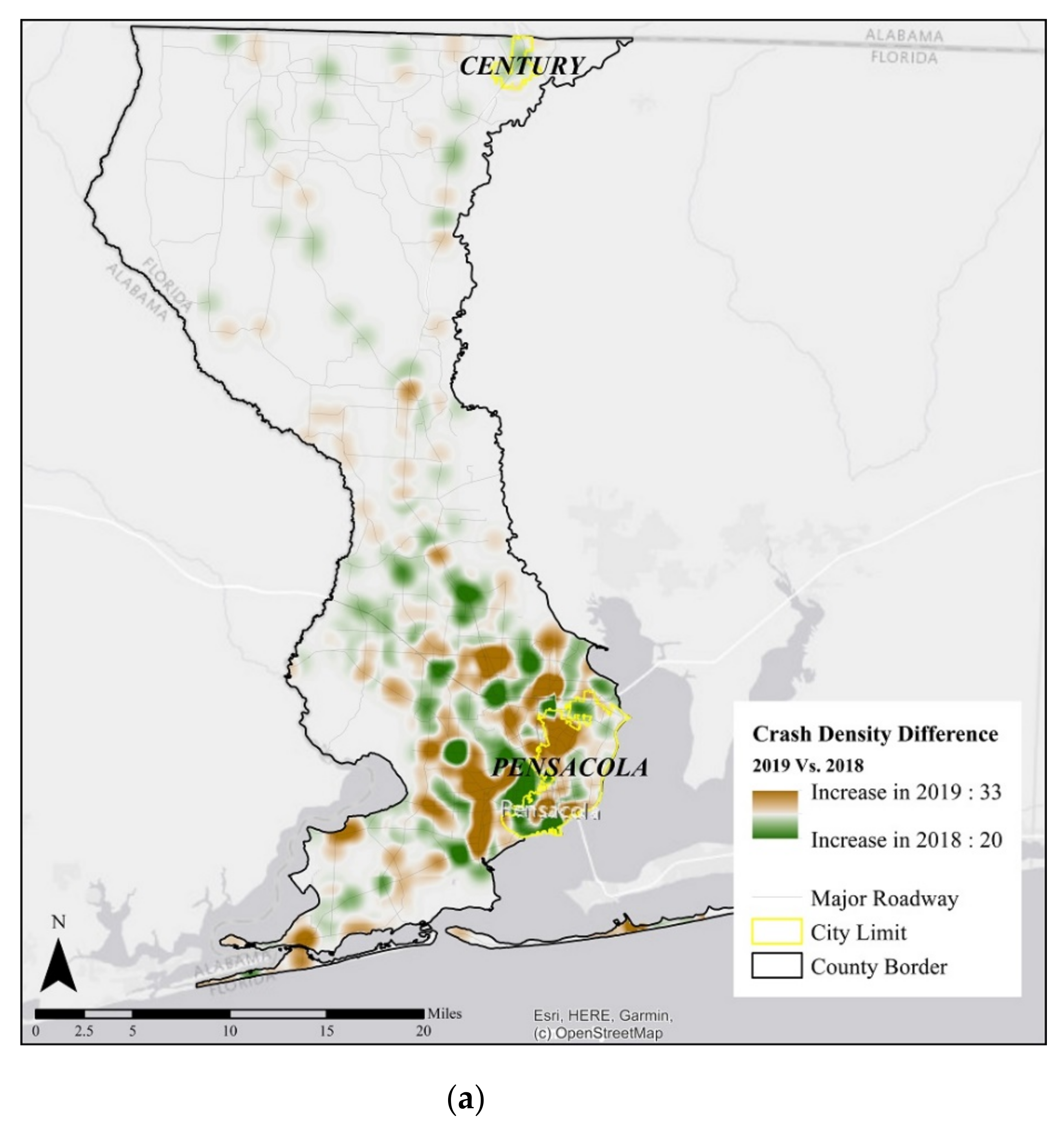
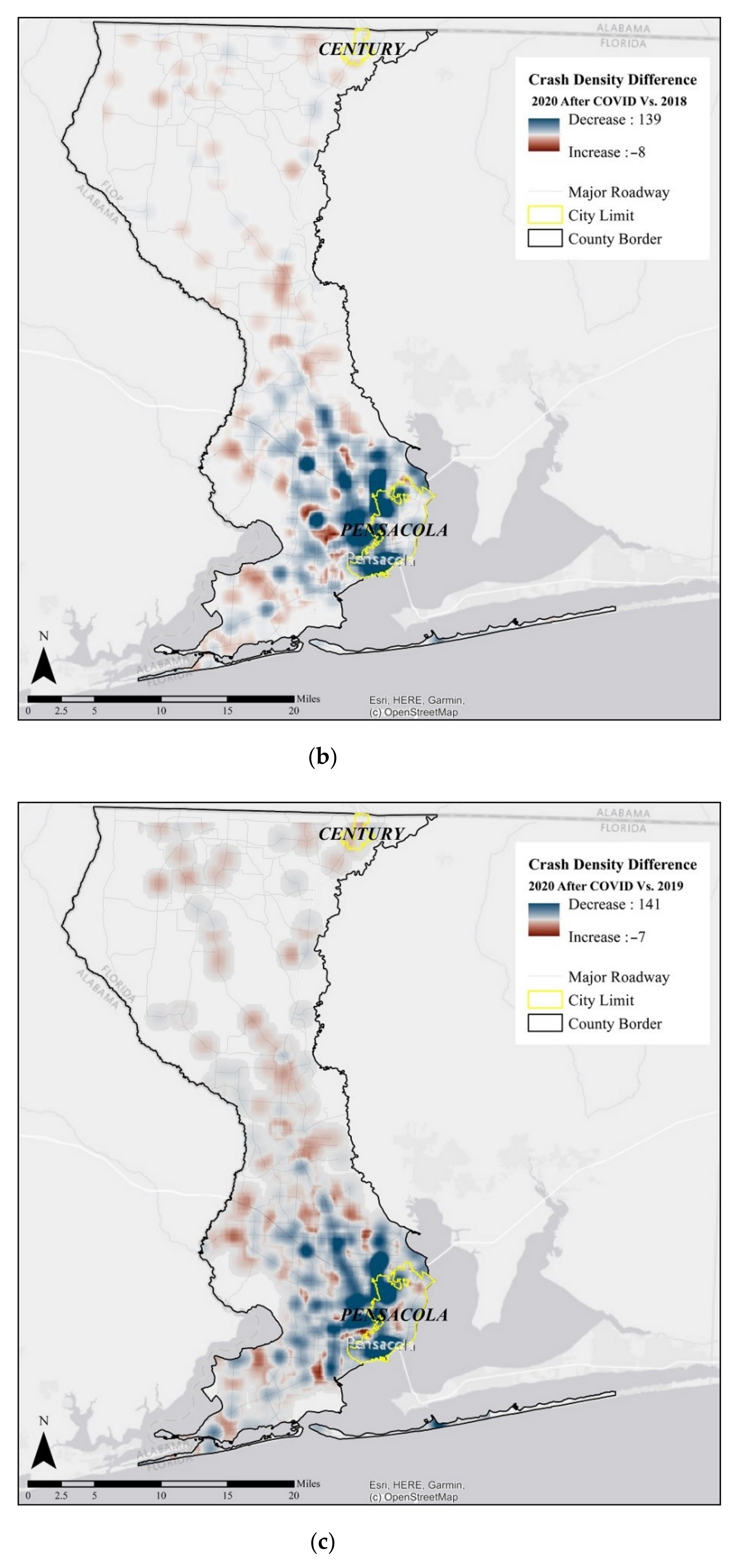
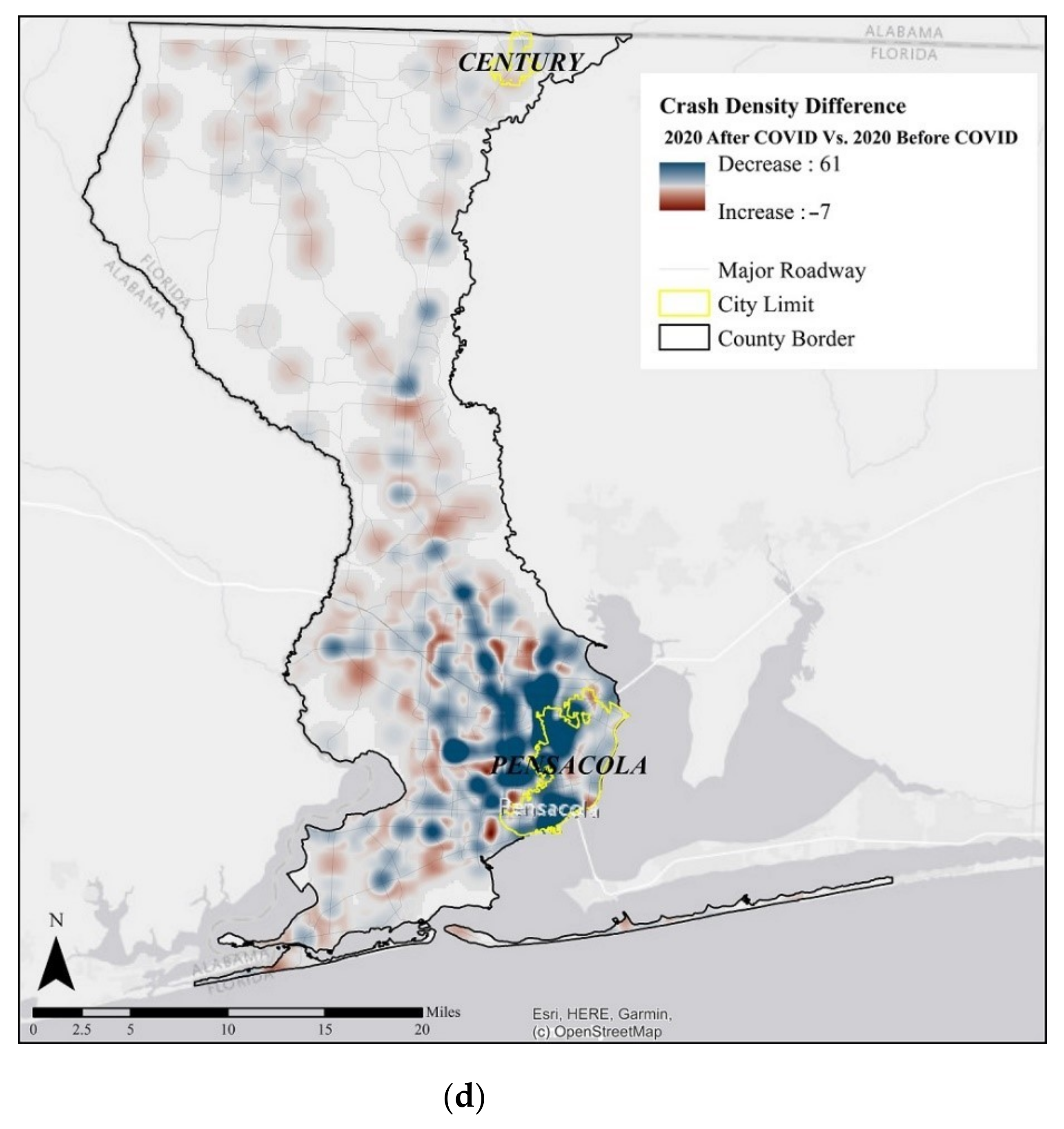
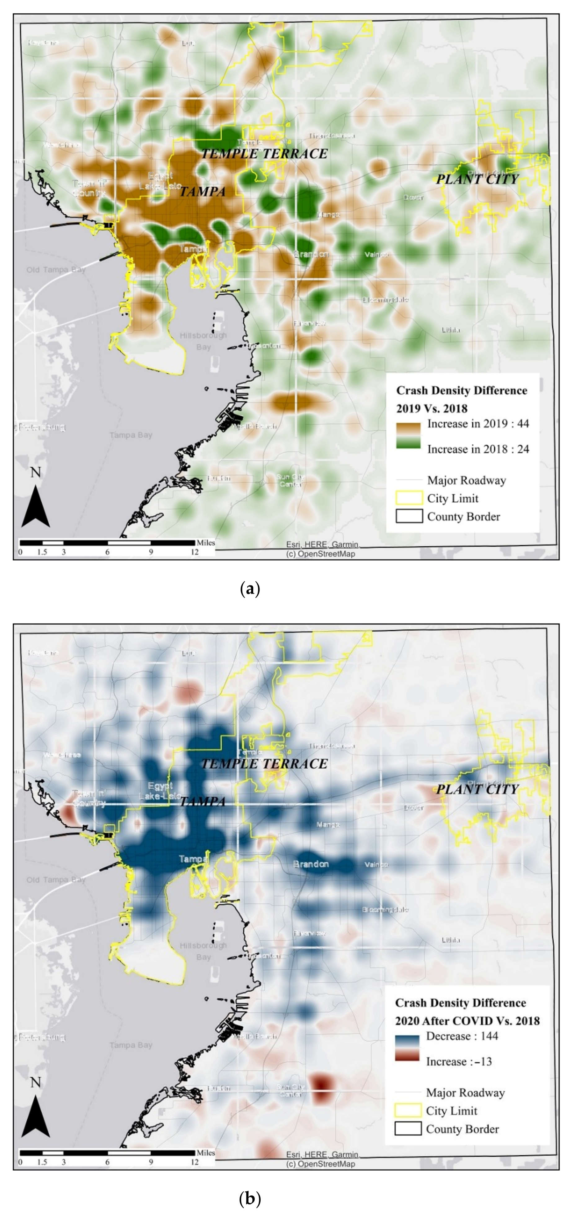
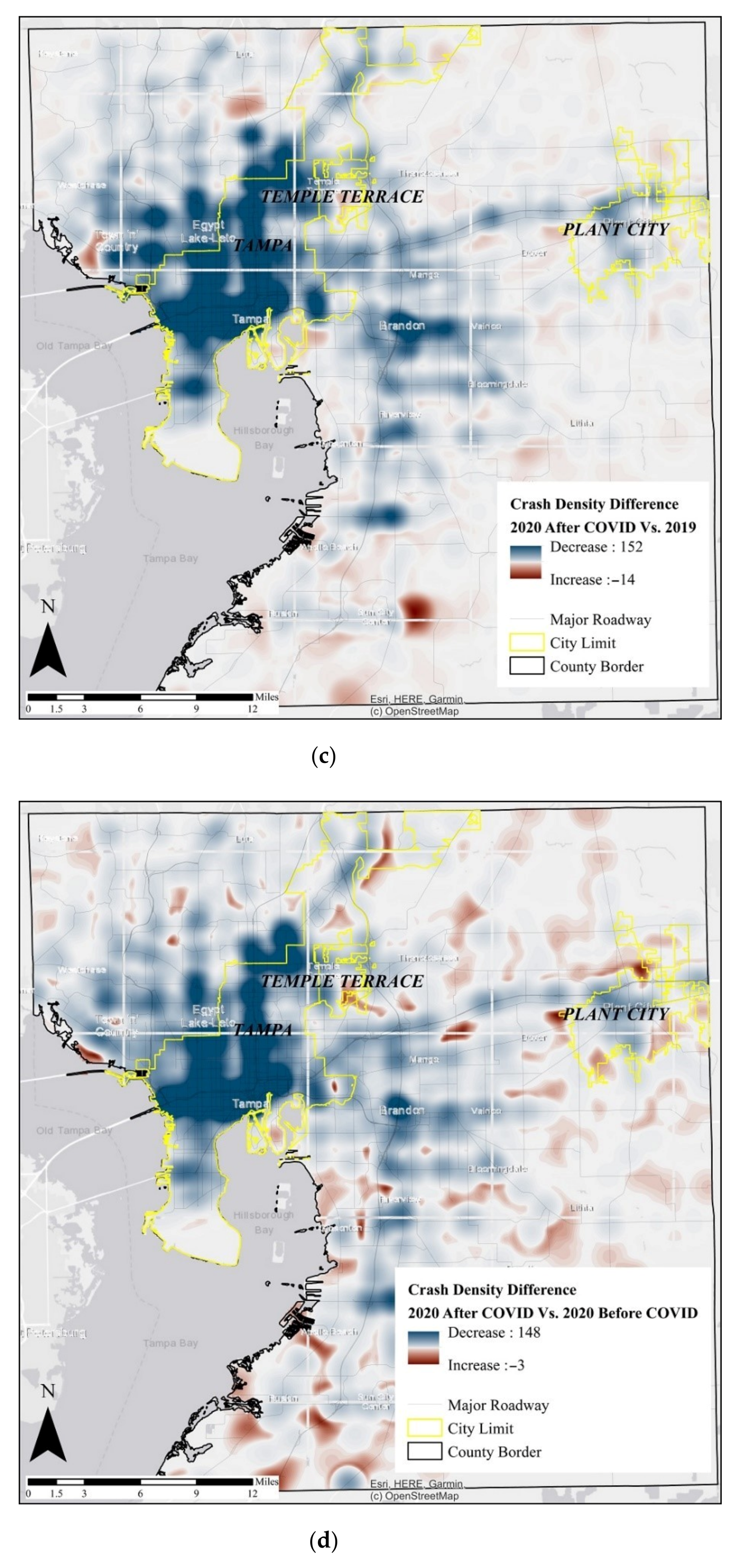
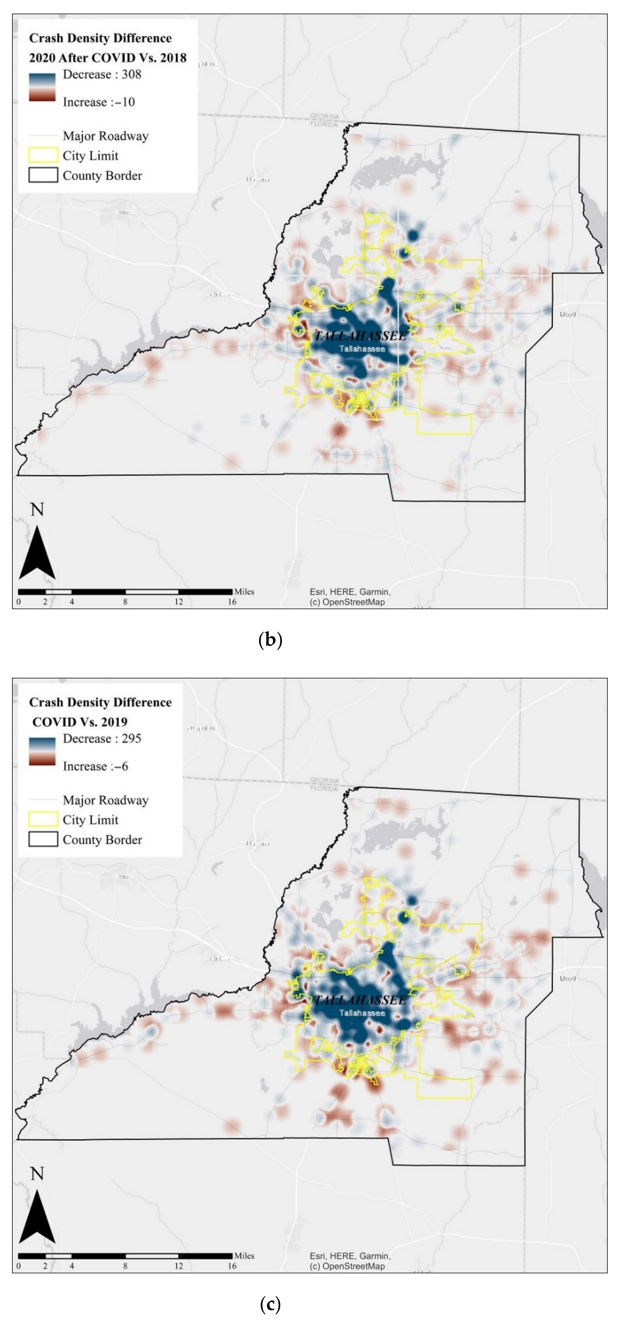
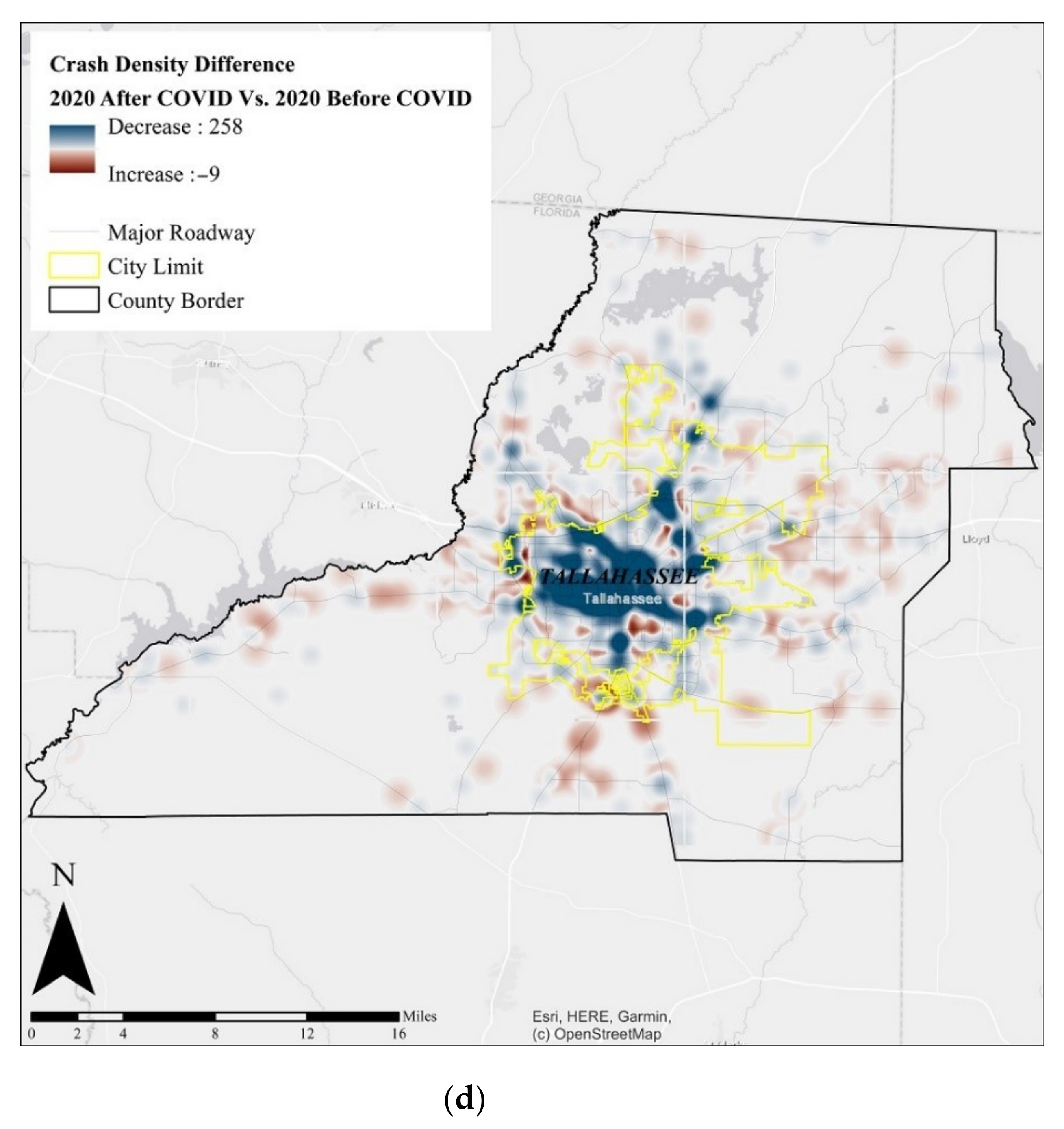
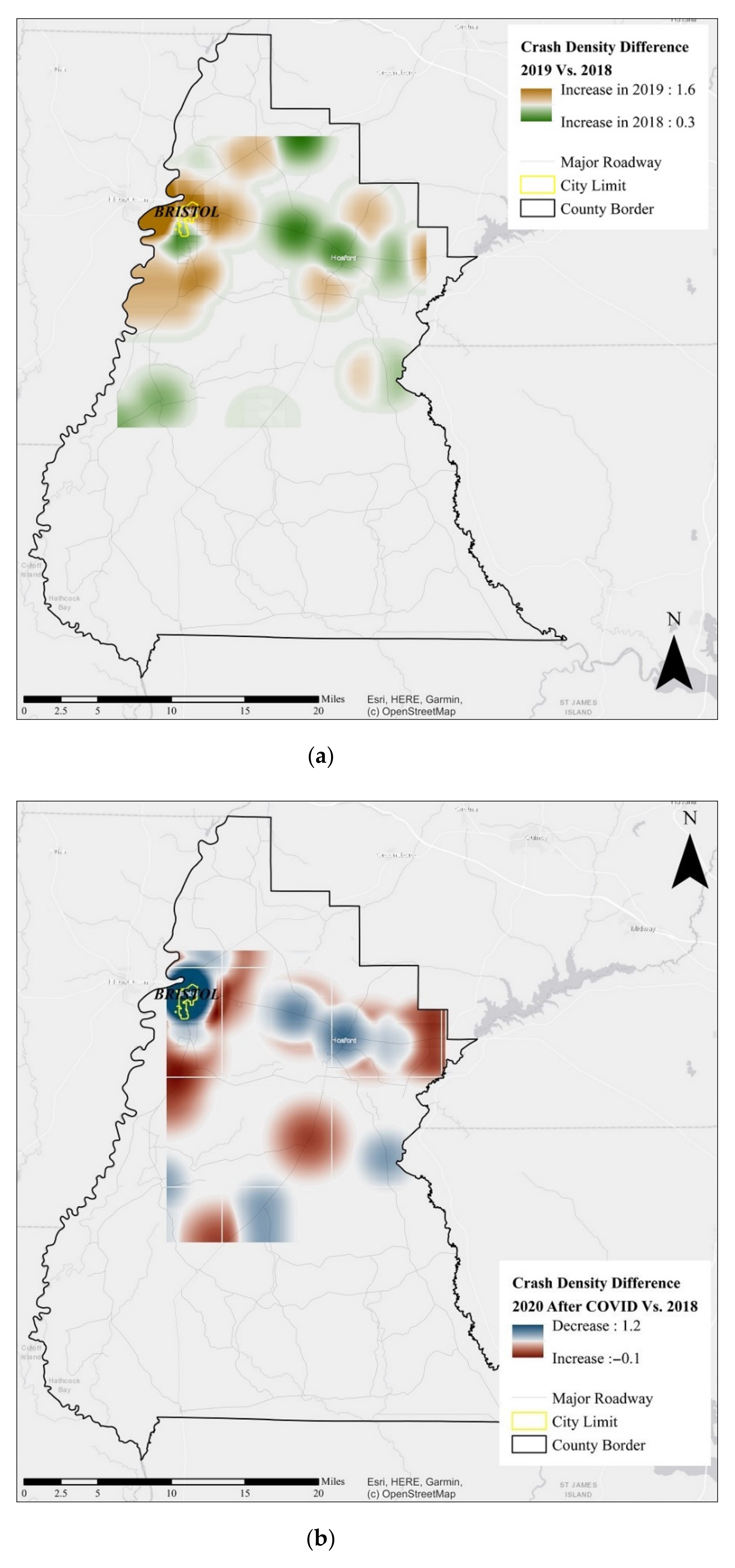
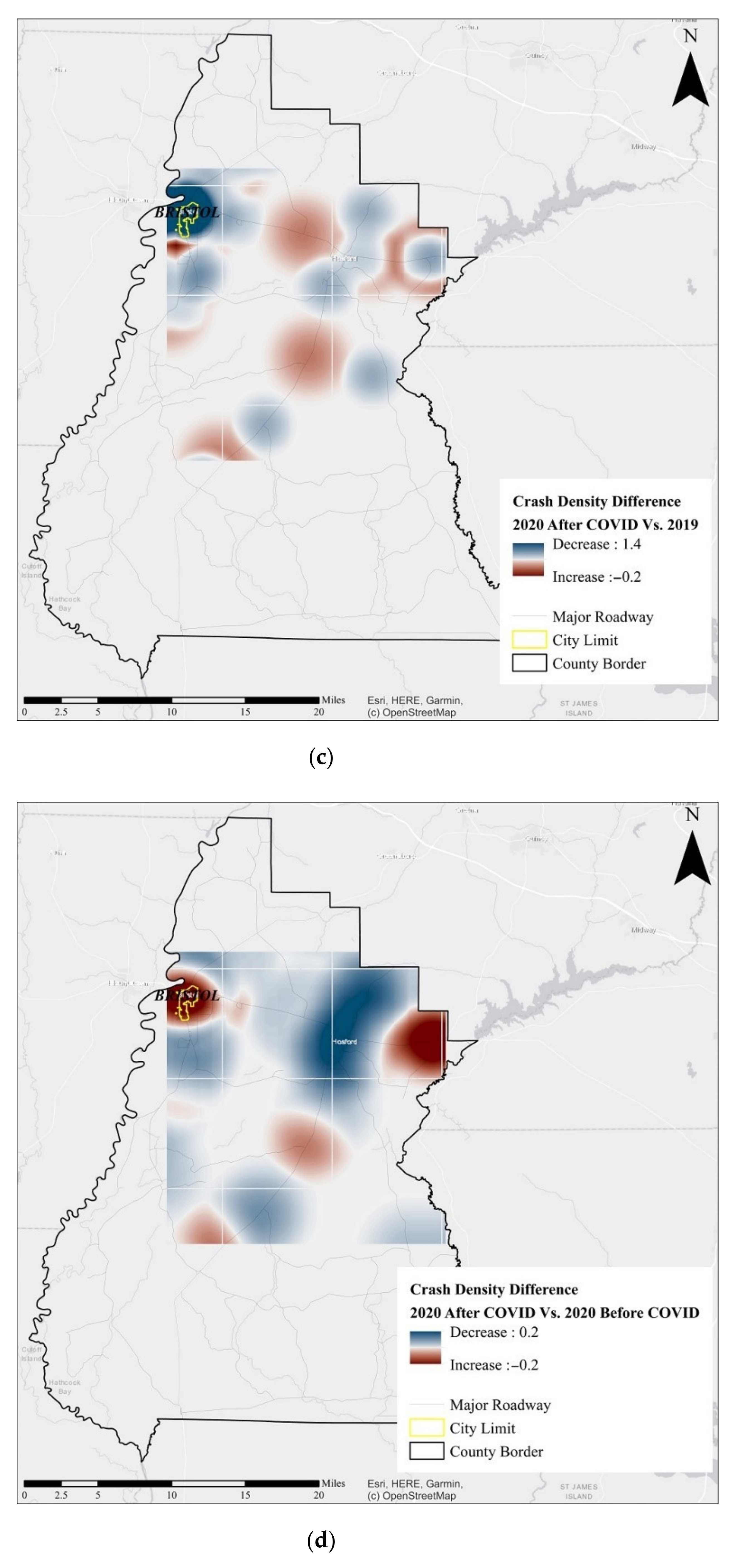
The COVID-19 pandemic has been affecting our lives drastically, and many people have been going about their daily lives remotely. With an extensive suite of spatial and statistical models, this study investigated the impacts of the noticeable change in mobility during the COVID-19 pandemic by analyzing its impact on the spatiotemporal patterns of crashes in four demographically different counties in Florida. We tried to evaluate how demographically different areas respond to policies that intend to reduce travel. The results obtained from the Kruskal–Wallis test indicate that COVID-19 conditions led to statistically significant reductions in crash densities in all counties. KDE-based spatial visualization reveals the highest crash density decreases mostly occurred within city limits regardless of different demographic characteristics of counties.
In order to examine the possibility of different responses to CCD from each County with various demographic and transportation-related factors, three separate negative binomial regression models have been developed. Among all these factors, the age-related variables have the most noticeable correlation with differences in crash density distribution during the COVID-19 pandemic. Although both are mid-size counties, NBR models for Escambia and Leon provide different results. The contribution of the youth (18–29) population ratio in the model reveals a percentage CCD change of 65% for every unit increase in the ratio of youth population living in census block groups of Leon County. This is mainly because of the county’s college-oriented nature.
Moreover, in Hillsborough County, we see interesting results regarding the aging (65+) population. The census block groups populated with more aging people seem to have a lower crash count decrease during the COVID-19 pandemic. This may possibly be due to the fact that these seniors did not change their daily travel habits during the COVID-19 pandemic. This may also show a need for the governments to teach them new technologies related to communication, shopping and medicine, so that they can avoid unnecessary trips. The findings for Leon County also reveal that remote working and other telecommunication methods, including e-shopping, decrease trip generation, particularly in the context of bike/walk mode choice “to-work” trips. This leads to more crash count decreases in areas that utilize these types of transportation modes due to COVID-19.

7. Limitations and Future Work

Since the topic is focusing on the crash count decrease during the COVID-19 pandemic, we needed to add some additional variables to the dataset to justify whether the changes in crash frequency and distribution are attributed to the changes in exposure (i.e., people travel less during the COVID-19 pandemic) or other issues. These required attributes include, but are not limited to, vehicle miles traveled (VMT), road network configuration, vehicle type, temporary local traffic management, land use, and trip generation. Further investigation of these additional attributes enables us to establish a cross-section model, including all counties in Florida in different time periods and considering all relevant built environment, transport system, population profile, and traffic factors.
There are several future research directions. For example, the proposed approach can be extended to evaluate the crash severities instead of counts to answer the following questions: How would a decrease in the total number of trips affect the severity of crashes? Would the drivers tend to drive at a higher speed in this case? Moreover, some findings of this research may be site-specific. Therefore, another interesting area of research is to expand this research into other counties. The current research disregarded the rural census block groups that experienced a negligible increase in the number of crashes compared to urban groups. It would be interesting to focus on these regions in more detail. The temporal results can also be utilized to interpret three-dimensional mapping of crash density differences in future research [77]. Furthermore, applying more advanced methods like propensity score matching (PSM) and empirical Bayes (EB) could provide reliable findings for a before-and-after comparison. Moreover, several researchers incorporated land use variables and assigning their contributions to the various types of crashes [78,79,80], so further investigation is required to assess how land use correlates with crash density patterns during the COVID-19 pandemic.

Author Contributions

The authors confirm contribution to the paper as follows: study conception and design: M.K., M.G., E.E.O. and M.B.U.; analysis and interpretation of results: M.K., M.G. and E.E.O.; manuscript preparation: M.K., M.G., E.E.O. and M.B.U. All authors reviewed the results. All authors have read and agreed to the published version of the manuscript.

Funding

This research did not receive any specific grant from funding agencies in the public, commercial, or not-for-profit sectors.

Data Availability Statement

Restrictions apply to the availability of these data. Data was obtained from Signal Four Analytics and are available at https://s4.geoplan.ufl.edu/ (accessed on 7 September 2021) with the permission of University of Florida.

Acknowledgments

The authors would like to thank the Florida Department of Transportation for providing data and valuable insight. The contents of this paper and discussion represent the authors’ opinion and do not reflect the official view of the Florida Department of Transportation.

Conflicts of Interest

The authors declare that they have no competing financial interest or personal relationships that could have appeared to influence the work reported in this paper.

References

  1. World Health Organization (WHO). 2021. Available online: https://www.who.int/emergencies/diseases/novel-coronavirus-2019 (accessed on 7 September 2021).
  2. Centers for Disease Control and Prevention (CDC). 2021. Available online: https://covid.cdc.gov/covid-data-tracker/#datatracker-home (accessed on 7 September 2021).
  3. Johns Hopkins University. Coronavirus COVID-19 Global Cases by the Center for Systems Science and Engineering (CSSE). Available online: https://www.arcgis.com/apps/opsdashboard/index.html#/bda7594740fd40299423467b48e9ecf6 (accessed on 5 October 2020).
  4. Ulak, M.B.; Ozguven, E.E.; Spainhour, L. Age-based stratification of drivers to evaluate the effects of age on crash involvement. Transp. Res. Procedia 2017, 22, 551–560. [Google Scholar] [CrossRef]
  5. Govindan, K.; Mina, H.; Alavi, B. A decision support system for demand management in healthcare supply chains considering the epidemic outbreaks: A case study of coronavirus disease 2019 (COVID-19). Transp. Res. Part E Logist. Transp. Rev. 2020, 138, 101967. [Google Scholar] [CrossRef] [PubMed]
  6. American Community Survey (ACS). Available online: https://www.census.gov/acs/www/data/data-tables-and-tools/data-profiles/ (accessed on 7 September 2021).
  7. Harbeck, E.L.; Glendon, A.I. Driver prototypes and behavioral willingness: Young driver risk perception and reported engagement in risky driving. J. Saf. Res. 2018, 66, 195–204. [Google Scholar] [CrossRef]
  8. Laflamme, L.; Hasselberg, M.; Kullgren, A.; Vaez, M. First car-to-car crashes involving young adult drivers: Main patterns and their relation to car and driver characteristics. Int. J. Inj. Control. Saf. Promot. 2006, 13, 179–186. [Google Scholar] [CrossRef] [PubMed]
  9. Mannering, F.; Bhat, C. Analytic methods in accident research: Methodological frontier and future directions. Anal. Methods Accid. Res. 2014, 1, 1–22. [Google Scholar] [CrossRef]
  10. Lord, D.; Mannering, F. The statistical analysis of crash-frequency data: A review and assessment of methodological alternatives. Transp. Res. Part A Policy Pract. 2010, 44, 291–305. [Google Scholar] [CrossRef] [Green Version]
  11. Abdel-Aty, M.A.; Radwan, A. Modeling traffic accident occurrence and involvement. Accid. Anal. Prev. 2000, 32, 633–642. [Google Scholar] [CrossRef]
  12. Ullman, D.S.; Ginis, I.; Huang, W.; Nowakowski, C.; Chen, X.; Stempel, P. Assessing the Multiple Impacts of Extreme Hurricanes in Southern New England, USA. Geosciences 2019, 9, 265. [Google Scholar] [CrossRef] [Green Version]
  13. Huang, H.; Abdel-Aty, M.A.; Darwiche, A.L. County-Level Crash Risk Analysis in Florida: Bayesian Spatial Modeling. Transp. Res. Rec. J. Transp. Res. Board 2010, 2148, 27–37. [Google Scholar] [CrossRef]
  14. Mousavi, S.M.; Zhang, Z.; Parr, S.A.; Pande, A.; Wolshon, B. Identifying High Crash Risk Highway Segments Using Jerk-Cluster Analysis. In Proceedings of the International Conference on Transportation and Development 2019: Smarter and Safer Mobility and Cities, Alexandria, Virginia, 9–12 June 2019. [Google Scholar]
  15. Mansourkhaki, A.; Karimpour, A.; Yazdi, H.S. Non-stationary concept of accident prediction. Proc. Inst. Civ. Eng.-Transp. 2017, 170, 140–151. [Google Scholar] [CrossRef]
  16. Lai, P.C.; Chan, W.Y. GIS for Road Accident Analysis in Hong Kong. Ann. GIS 2004, 10, 58–67. [Google Scholar] [CrossRef]
  17. Manap, N.; Borhan, M.; Yazid, M.; Hambali, M.; Rohan, A. Determining Spatial Patterns of Road Accidents at Expressway by Applying Getis-Ord Gi* Spatial Statistic. Int. J. Recent Technol. Eng. 2019, 8, 345–350. [Google Scholar] [CrossRef]
  18. Rogerson, P.A. Maximum Getis-Ord Statistic Adjusted for Spatially Autocorrelated Data. Geogr. Anal. 2014, 47, 20–33. [Google Scholar] [CrossRef]
  19. Law, J.; Quick, M.; Chan, P.W. Analyzing Hotspots of Crime Using a Bayesian Spatiotemporal Modeling Approach: A Case Study of Violent Crime in the Greater Toronto Area. Geogr. Anal. 2014, 47, 1–19. [Google Scholar] [CrossRef]
  20. Cheng, S.; Lu, F.; Peng, P.; Wu, S. Short-term traffic forecasting: An adaptive ST-KNN model that considers spatial heterogeneity. Comput. Environ. Urban Syst. 2018, 71, 186–198. [Google Scholar] [CrossRef]
  21. Han, Q.; Zhu, Y.; Zeng, L.; Ye, L.; He, X.; Liu, X.; Wu, H.; Zhu, Q. A Road Hotspots Identification Method Based on Natural Nearest Neighbor Clustering. In Proceedings of the 2015 IEEE 18th International Conference on Intelligent Transportation Systems, Las Palmas de Gran Canaria, Spain, 15–18 September 2015; pp. 553–557. [Google Scholar] [CrossRef]
  22. Abdulhafedh, A. Identifying Vehicular Crash High Risk Locations along Highways via Spatial Autocorrelation Indices and Kernel Density Estimation. World J. Eng. Technol. 2017, 05, 198–215. [Google Scholar] [CrossRef] [Green Version]
  23. Zhang, Z.; Ming, Y.; Song, G. A New Approach to Identifying Crash Hotspot Intersections (CHIs) Using Spatial Weights Matrices. Appl. Sci. 2020, 10, 1625. [Google Scholar] [CrossRef] [Green Version]
  24. Prasannakumar, V.; Vijith, H.; Charutha, R.; Geetha, N. Spatio-Temporal Clustering of Road Accidents: GIS Based Analysis and Assessment. Procedia-Soc. Behav. Sci. 2011, 21, 317–325. [Google Scholar] [CrossRef] [Green Version]
  25. Dai, D.; Taquechel, E.; Steward, J.; Strasser, S. The impact of built environment on pedestrian crashes and the identifica-tion of crash clusters on an urban university campus. West. J. Emerg. Med. 2010, 11, 294–301. [Google Scholar]
  26. Borruso, G. Network Density Estimation: A GIS Approach for Analysing Point Patterns in a Network Space. Trans. GIS 2008, 12, 377–402. [Google Scholar] [CrossRef]
  27. Chow, T.E.; Choi, Y.; Yang, M.; Mills, D.; Yue, R. Geographic pattern of human mobility and COVID-19 before and after Hubei lockdown. Ann. GIS 2020, 27, 241–243. [Google Scholar] [CrossRef]
  28. Ghorbanzadeh, M.; Kim, K.; Ozguven, E.E.; Horner, M.W. Spatial Accessibility Assessment of COVID-19 Patients to Healthcare Facilities: A Case Study of Florida. Travel Behav. Soc. 2021, 24, 95–101. [Google Scholar] [CrossRef] [PubMed]
  29. Kim, K.; Ghorbanzadeh, M.; Horner, M.H.; Ozguven, E.E. Identifying areas of potential critical healthcare shortages: A case study of spatial accessibility to ICU beds during the COVID-19 pandemic in Florida. Transp. Policy 2021, 110, 478–486. [Google Scholar] [CrossRef] [PubMed]
  30. Kerlin, K. California COVID-19 Traffic Report Finds Silver Lining. 2020. Available online: https://www.ucdavis.edu/coronavirus/news/california-covid-19-traffic-report (accessed on 7 September 2021).
  31. Bain, M. COVID-19 Has Halved California’s Traffic Accidents. 2020. Available online: https://qz.com/1840736/coronavirus-reduces-california-traffic-accidents-by-half/ (accessed on 7 September 2021).
  32. Oguzoglu, U. COVID-19 Lockdowns and Decline in Traffic Related Deaths and Injuries; IZA Discuss, Institute of Labor Economics. Pap., No. 13278; University of Manitoba and IZA: Winnipeg, MB, Canada, 2020. [Google Scholar]
  33. Brodeur, A.; Cook, N.; Wright, T. On the Effects of COVID-19 Safer-At-Home Policies on Social Distancing, Car Crashes and Pollution; IZA Discuss, Institute of Labor Economics. Pap., No. 13255; University of Ottawa and IZA: Ottawa, ON, Canada, 2020. [Google Scholar]
  34. Kirby, B. Coronavirus Side Effect—Alabama Highway Traffic Wrecks Plummet. 2020. Available online: https://www.fox10tv.com/news/coronavirus/coronavirus-side-effect-alabama-highway-traffic-wrecks-plummet/article_3d5df80e-8a74-11ea-b0c7-db9eea522371.html (accessed on 7 September 2021).
  35. NCDOT. Effect of the COVID-19 Crisis on Traffic Crashes in North Carolina. 2020. Available online: https://connect.ncdot.gov/resources/safety/CrashDataandTeaasSystem/COVID-19_ImpactOnTrafficCrashes.pdf (accessed on 7 September 2021).
  36. National Police Foundation. Assessing the Impact of COVID-19 and Community Responses on Traffic Crashes and Fatali-ties. 2020. Available online: https://www.policefoundation.org/assessing-the-impact-of-covid-19-and-community-responses-on-traffic-crashes-and-fatalities/ (accessed on 7 September 2021).
  37. Farrell, C.L. COVID-19 Order Leads to Fewer Indiana Traffic Accidents. 2020. Available online: https://www.cflblaw.com/2020/04/covid-indiana-car-accidents/ (accessed on 7 September 2021).
  38. Parr, S.; Wolshon, B.; Renne, J.; Murray-Tuite, P.; Kim, K. Traffic Impacts of the COVID-19 Pandemic: Statewide Analysis of Social Separation and Activity Restriction. Nat. Hazards Rev. 2020, 21, 04020025. [Google Scholar] [CrossRef]
  39. Xiong, C.; Hu, S.; Yang, M.; Luo, W.; Zhang, L. Mobile device data reveal the dynamics in a positive relationship between human mobility and COVID-19 infections. Proc. Natl. Acad. Sci. USA 2020, 117, 27087–27089. [Google Scholar] [CrossRef] [PubMed]
  40. Chan, H.F.; Skali, A.; Savage, D.A.; Stadelmann, D.; Torgler, B. Risk attitudes and human mobility during the COVID-19 pandemic. Sci. Rep. 2020, 10, 19931. [Google Scholar] [CrossRef]
  41. Borkowski, P.; Jażdżewska-Gutta, M.; Szmelter-Jarosz, A. Lockdowned: Everyday mobility changes in response to COVID-19. J. Transp. Geogr. 2020, 90, 102906. [Google Scholar] [CrossRef]
  42. Rotem-Mindali, O.; Salomon, I. The impacts of E-retail on the choice of shopping trips and delivery: Some preliminary findings. Transp. Res. Part A Policy Pract. 2007, 41, 176–189. [Google Scholar] [CrossRef]
  43. Shilling, F.; Waetjen, D. Impact of COVID19 Mitigation on Numbers and Costs of California Traffic Crashes Impact of COVID19 Mitigation on California Traffic Crashes; Road Ecology Center, UC Davis: Davis, CA, USA, 2020; Volume 2020. [Google Scholar]
  44. Chang, M.-C.; Kahn, R.; Li, Y.-A.; Lee, C.-S.; Buckee, C.O.; Chang, H.-H. Variation in human mobility and its impact on the risk of future COVID-19 outbreaks in Taiwan. BMC Public Health 2021, 21, 226. [Google Scholar] [CrossRef]
  45. Doucette, M.L.; Tucker, A.; Auguste, M.E.; Watkins, A.; Green, C.; Pereira, F.E.; Borrup, K.T.; Shapiro, D.; Lapidus, G. Initial impact of COVID-19′s stay-at-home order on motor vehicle traffic and crash patterns in Connecticut: An interrupted time series analysis. Inj. Prev. 2020, 27, 3–9. [Google Scholar] [CrossRef] [PubMed]
  46. Brimley, B.K.; Saito, M.; Schultz, G.G. Calibration of Highway Safety Manual Safety Performance Function. Transp. Res. Rec. J. Transp. Res. Board 2012, 2279, 82–89. [Google Scholar] [CrossRef]
  47. Jonsson, T.; Lyon, C.; Ivan, J.N.; Washington, S.P.; van Schalkwyk, I.; Lord, D. Differences in the Performance of Safety Performance Functions Estimated for Total Crash Count and for Crash Count by Crash Type. Transp. Res. Rec. J. Transp. Res. Board 2009, 2102, 115–123. [Google Scholar] [CrossRef]
  48. Hayden, A.; Tight, M.; Burrow, M. Is Reducing Car Use a Utopian Vision? Transp. Res. Procedia 2017, 25, 3944–3956. [Google Scholar] [CrossRef]
  49. Wang, Q.; Sun, H. Traffic Structure Optimization in Historic Districts Based on Green Transportation and Sustainable Development Concept. Adv. Civ. Eng. 2019, 2019, 9196263. [Google Scholar] [CrossRef]
  50. Hongjun, L. Study on Sustainable Development Highway Traffic. In Proceedings of the 2nd International Conference on Civil Architecture and Energy Science (CAES 2020), Changchun, China, 20–22 March 2020; Volume 165, p. 04043. [Google Scholar] [CrossRef]
  51. Geels, F.W. A socio-technical analysis of low-carbon transitions: Introducing the multi-level perspective into transport studies. J. Transp. Geogr. 2012, 24, 471–482. [Google Scholar] [CrossRef]
  52. Beck, M.J.; Hensher, D.A.; Wei, E. Slowly coming out of COVID-19 restrictions in Australia: Implications for working from home and commuting trips by car and public transport. J. Transp. Geogr. 2020, 88, 102846. [Google Scholar] [CrossRef]
  53. Omer, I.; Gitelman, V.; Rofè, Y.; Lerman, Y.; Kaplan, N.; Doveh, E. Evaluating Crash Risk in Urban Areas Based on Vehicle and Pedestrian Modeling. Geogr. Anal. 2017, 49, 387–408. [Google Scholar] [CrossRef]
  54. Florida’s Signal Four Analytics. 2020. Available online: https://s4.geoplan.ufl.edu/ (accessed on 7 September 2021).
  55. Saeed, T.U.; Nateghi, R.; Hall, T.; Waldorf, B.S. Statistical Analysis of Area-wide Alcohol-related Driving Crashes: A Spatial Econometric Approach. Geogr. Anal. 2019, 52, 394–417. [Google Scholar] [CrossRef]
  56. Pulugurtha, S.S.; Krishnakumar, V.K.; Nambisan, S.S. New methods to identify and rank high pedestrian crash zones: An illustration. Accid. Anal. Prev. 2007, 39, 800–811. [Google Scholar] [CrossRef]
  57. Plug, C.; Xia, J.; Caulfield, C. Spatial and temporal visualisation techniques for crash analysis. Accid. Anal. Prev. 2011, 43, 1937–1946. [Google Scholar] [CrossRef]
  58. Ulak, M.B.; Ozguven, E.E.; Spainhour, L.; Vanli, O.A. Spatial investigation of aging-involved crashes: A GIS-based case study in Northwest Florida. J. Transp. Geogr. 2016, 58, 71–91. [Google Scholar] [CrossRef]
  59. Ghorbanzadeh, M.; Koloushani, M.; Ulak, M.B.; Ozguven, E.E.; Jouneghani, R.A.; Arghandeh, R. Statistical and Spatial Analysis of Hurricane-induced Roadway Closures and Power Outages. Energies 2020, 13, 1098. [Google Scholar] [CrossRef] [Green Version]
  60. Vemulapalli, S.S.; Ulak, M.; Ozguven, E.E.; Sando, T.; Horner, M.W.; AbdelRazig, Y.; Moses, R. GIS-based Spatial and Temporal Analysis of Aging-Involved Accidents: A Case Study of Three Counties in Florida. Appl. Spat. Anal. Policy 2016, 10, 537–563. [Google Scholar] [CrossRef]
  61. Jiang, X.; Yan, X.; Huang, B.; Richards, S.H. Influence of Curbs on Traffic Crash Frequency on High-Speed Roadways. Traffic Inj. Prev. 2011, 12, 412–421. [Google Scholar] [CrossRef] [PubMed]
  62. Ehrlich, P.F.; Brown, J.K.; Sochor, M.R.; Wang, S.C.; Eichelberger, M.E. Factors influencing pediatric Injury Severity Score and Glasgow Coma Scale in pediatric automobile crashes: Results from the Crash Injury Research Engineering Network. J. Pediatr. Surg. 2006, 41, 1854–1858. [Google Scholar] [CrossRef]
  63. Bakhshi, A.K.; Ahmed, M.M. Utilizing black-box visualization tools to interpret non-parametric real-time risk assessment models. Transp. A Transp. Sci. 2020, 17, 739–765. [Google Scholar] [CrossRef]
  64. Ye, X.; Wang, K.; Zou, Y.; Lord, D. A semi-nonparametric Poisson regression model for analyzing motor vehicle crash data. PLoS ONE 2018, 13, e0197338. [Google Scholar] [CrossRef]
  65. Nilsson, P.; Nilsson, S. Application of Poisson Regression on Traffic Safety; Royal Institute of Technology: Stockholm, Sweden, 2015. [Google Scholar]
  66. Mohammadi, M.A.; Samaranayake, V.A.; Bham, G. Crash frequency modeling using negative binomial models: An application of generalized estimating equation to longitudinal data. Anal. Methods Accid. Res. 2014, 2, 52–69. [Google Scholar] [CrossRef]
  67. Elvik, R.; Goel, R. Safety-in-numbers: An updated meta-analysis of estimates. Accid. Anal. Prev. 2019, 129, 136–147. [Google Scholar] [CrossRef]
  68. Arentze, T.; Borgers, A.; Timmermans, H. A model of multi-purpose shopping trip behavior. Pap. Reg. Sci. 1993, 72, 239–256. [Google Scholar] [CrossRef] [Green Version]
  69. Russo, F.; Comi, A. The Simulation of Shopping Trips at Urban Scale: Attraction Macro-Model. Procedia-Soc. Behav. Sci. 2012, 39, 387–399. [Google Scholar] [CrossRef]
  70. Wang, L.; Abdel-Aty, M.; Lee, J.; Shi, Q. Analysis of real-time crash risk for expressway ramps using traffic, geometric, trip generation, and socio-demographic predictors. Accid. Anal. Prev. 2017, 122, 378–384. [Google Scholar] [CrossRef]
  71. Naderan, A.; Shahi, J. Aggregate crash prediction models: Introducing crash generation concept. Accid. Anal. Prev. 2010, 42, 339–346. [Google Scholar] [CrossRef]
  72. Shariat-Mohaymany, A.; Shahri, M.; Mirbagheri, B.; Matkan, A.A. Exploring Spatial Non-Stationarity and Varying Relationships between Crash Data and Related Factors Using Geographically Weighted Poisson Regression. Trans. GIS 2014, 19, 321–337. [Google Scholar] [CrossRef]
  73. Chung, Y.-S. Factor complexity of crash occurrence: An empirical demonstration using boosted regression trees. Accid. Anal. Prev. 2012, 61, 107–118. [Google Scholar] [CrossRef]
  74. Chen, F.; Chen, S.; Ma, X. Analysis of hourly crash likelihood using unbalanced panel data mixed logit model and real-time driving environmental big data. J. Saf. Res. 2018, 65, 153–159. [Google Scholar] [CrossRef]
  75. Iwamoto, D.K.; Liu, W.M. The impact of racial identity, ethnic identity, Asian values, and race-related stress on Asian Americans and Asian international college students’ psychological well-being. J. Couns. Psychol. 2010, 57, 79–91. [Google Scholar] [CrossRef] [Green Version]
  76. De Vos, J. The effect of COVID-19 and subsequent social distancing on travel behavior. Transp. Res. Interdiscip. Perspect. 2020, 5, 100121. [Google Scholar] [CrossRef] [PubMed]
  77. Nakaya, T.; Yano, K. Visualising Crime Clusters in a Space-time Cube: An Exploratory Data-analysis Approach Using Space-time Kernel Density Estimation and Scan Statistics. Trans. GIS 2010, 14, 223–239. [Google Scholar] [CrossRef]
  78. Kim, K.; Pant, P.; Yamashita, E. Accidents and Accessibility: Measuring Influences of Demographic and Land Use Variables in Honolulu, Hawaii. Transp. Res. Rec. J. Transp. Res. Board 2010, 2147, 9–17. [Google Scholar] [CrossRef]
  79. Ouyang, Y.; Bejleri, I. Geographic Information System–Based Community-Level Method to Evaluate the Influence of Built Environment on Traffic Crashes. Transp. Res. Rec. J. Transp. Res. Board 2014, 2432, 124–132. [Google Scholar] [CrossRef]
  80. Xie, B.; An, Z.; Zheng, Y.; Li, Z. Incorporating transportation safety into land use planning: Pre-assessment of land use conversion effects on severe crashes in urban China. Appl. Geogr. 2018, 103, 1–11. [Google Scholar] [CrossRef]
Figure 1. Study area.
Futuretransp 01 00023 g001
Figure 2. Histogram for crash count decreases (CCD).
Futuretransp 01 00023 g002aFuturetransp 01 00023 g002b
Figure 3. Crash density differences in Escambia County. (a) Between 2018 and 2019; (b) between 2020 After COVID-19 and 2018; (c) between 2020 After COVID-19 and 2019; and (d) between 2020 After COVID-19 and 2020 before COVID-19.
Futuretransp 01 00023 g003aFuturetransp 01 00023 g003bFuturetransp 01 00023 g003c
Figure 4. Crash density differences in Hillsborough County. (a) Between 2018 and 2019; (b) between 2020 After COVID-19 and 2018; (c) between 2020 after COVID-19 and 2019; and (d) between 2020 after COVID-19 and 2020 before COVID-19.
Futuretransp 01 00023 g004aFuturetransp 01 00023 g004b
Figure 5. Crash density differences in Leon County. (a) between 2018 and 2019; (b) between 2020 After COVID-19 and 2018; (c) between 2020 after COVID-19 and 2019; and (d) between 2020 after COVID-19 and 2020 before COVID-19.
Futuretransp 01 00023 g005aFuturetransp 01 00023 g005bFuturetransp 01 00023 g005c
Figure 6. Crash density differences in Liberty County. (a) between 2018 and 2019, (b) between 2020 After COVID-19 and 2018, (c) between 2020 after COVID-19 and 2019, and (d) between 2020 after COVID-19 and 2020 before COVID-19.
Futuretransp 01 00023 g006aFuturetransp 01 00023 g006b
Figure 7. Time series. (a) Escambia County; (b) Hillsborough County; and (c) Leon County.
Futuretransp 01 00023 g007
Figure 8. Crash count difference (CDC). (a) Escambia County; (b) Hillsborough County; (c) Leon County; and (d) Liberty County.
Futuretransp 01 00023 g008
Table 1. Descriptive statistics associated with selected counties.
CharacteristicsCounty
EscambiaHillsboroughLeonLiberty
Total number of census block group1918811776
Area [ac] 559,808.2810,059.8449,144.7539,598.5
Total populationSum311,5221,378,883288,1028365
Mean16311565.11627.71394.2
STD961.51230.3850.9665.1
Asian PopulationAverage Percentage2.8%3.3%2.9%0.1%
Sum988655,15710,10720
Mean51.862.657.13.3
STD88.4129.9104.25.2
Hispanic or Latino PopulationAverage Percentage5.4%27.1%6.2%4.9%
Sum17,293386,47818,050484
Mean90.5438.7101.980.6
STD127.8466.2106.8112.9
Population with a DisabilitiesAverage Percentage7.7%6.2%6.1%20.2%
Sum23,02578,54817,077800
Mean120.589.196.5133.3
STD88.574.280.948.1
Aging (+65) PopulationAverage Percentage17.3%15.5%13.5%17.9%
Sum50,472189,67635,7001305
Mean264.2215.3201.6217.5
STD172.6195.1159.590
Young (18–29) PopulationAverage Percentage18.3%16.3%29.8%17.1%
Sum62,136235,38087,4221514
Mean325.3267.1493.9252.3
STD458.6333.4522.6172.4
Average Household SizeSum465.92285419.417.4
Mean2.42.62.372.91
STD0.460.60.550.32
Household below Poverty LevelSum14,23873,47421,755375
Mean74.583.4122.962.5
STD69.284.8149.816.9
Use of Walk/BikeSum408213,676423325
Mean21.415.523.94.1
STD77.834.742.49.3
Total Enrollment22,38889,40964,8910
Percentage to Total Population7%6%23%0%
Curfew starting dateNA13 April25 MarchNA
Time-21:00–5:0023:00–5:00-
Table 2. Crash data and Average Annual Daily Traffic (AADT).
Time PeriodEscambiaHillsboroughLeonLiberty
CountChangeCountChangeCountChangeCountChange
Crash2020 After COVID *1480-5032-1078-20-
2018 **244239.4%11,13054.8%282961.9%2725.9%
2019253941.7%11,11254.7%270260.1%3441.2%
2020 Before COVID ***219432.5%10,47552%256458%3339.4%
AADT201913,65222,80414,6282651
202013,05119,78112,9002481
* 15 March until 2 June 2020 during COVID-19 pandemic. ** 15 March until 2 June 2018 (consider the same period of time in 2019). *** 26 December 2019 until 14 March 2020 before COVID-19 pandemic.
Table 3. Description of variables.
Predictor VariableDescription
Total Population [/104]Total population in census block group
Average Household SizeAverage Household Size of Occupied Housing Units by Tenure
African American (RP)Ratio of black or African American population to total population
Asian (RP)Ratio of Asian population to total population
Hispanic or Latino (RP)Ratio of Hispanic or Latino population to total population
Young (18–29) (RP)Ratio of young (18–29) population to total population
Aging (65+) (RP)Ratio of aging (65+) population to total population
Population with a Disability (RP)Ratio of the population (20–64) years with a disability to total population
Use of Walk/Bike for (RT)Ratio of use of walk/bike to total number of transportation to work
Households below Poverty (RH)Ratio of households with income below poverty level to total number household
CCD (Dependent Variable)Crash count decrease in each census block group during COVID-19 pandemic
Table 4. Kruskal–Wallis test results.
CountyPair of Comparison
Vs.MeanSD χ 2 dfp-Value
Escambia2020 After COVID *2.1185.281
2020 before COVID **3.2559.16327,98913,898≈0
2019 ***3.78711.46128,14514,757≈0
20183.63411.03928,51114,871≈0
Hillsborough2020 After COVID3.9137.212
2020 before COVID8.82818.93348,79937,374≈0
20199.30619.6448,94438,026≈0
20188.70218.09849,08038,566≈0
Leon2020 After COVID1.4334.337
2020 before COVID3.77715.87843,33420,210≈0
20193.80315.87442,23619,136≈0
20183.64615.50242,14118,830≈0
Liberty2020 After COVID0.0400.083
2020 before COVID0.0630.0852,03645,836≈0
20190.0770.22638,97826,677≈0
20180.0630.1937,48619,918≈0
* 15 March until 2 June 2020 during COVID-19 condition. ** 26 December 2019 until 14 March 2020 before COVID-19 condition. *** 15 March until 2 June 2018 (consider the same period of time in 2019).
Table 5. Categorized crash count decrease during COVID-19 in each county.
Range of DecreaseNumber of Census Block
EscambiaHillsboroughLeonLiberty
<0 *32(16.8%) **96(10.9%)17(9.6%)1(16.7%)
0–10122(64.2%)620(70.6%)111(62.7%)5(83.3%)
11–5034(17.9%)151(17.2%)48(27.1%)0(0.0%)
51–1001(0.5%)9(1.0%)0(0.0%)0(0.0%)
>1001(0.5%)2(0.2%)1(0.6%)0(0.0%)
* Crash count increases during COVID-19 in census block group. ** Numbers in parentheses present the percentage to the total number of census block groups in each county.
Table 6. Negative binomial regression analysis results, (a) Escambia County, (b) Hillsborough County, and (c) Leon County.
RegressorsEscambia CountyHillsborough CountyLeon County
βSEp90%βSEp90%βSEp90%
Intercept3.520.813 0 3.250.318 0 3.7520.48 0
Total Population [/104]2.8171 × 10−40.011.333 × 10−5 0 2.7719 × 10−50.003
Asian (RP *)2.810.020.163−0.1958 × 10−30.811−4.5080.0180.014
Hispanic or Latino (RP *)−0.6420.0150.6661.0052 × 10−3 0 0.3770.0140.789
Average Household Size−1.0290.263 0 −0.6520.091 0 −0.8780.186 0
Youth (18–29) (RP *)−1.5970.010.108−0.2995 × 10−30.5120.650.0030.065
Aging (65+) (RP *)−0.3290.0130.805−1.614 × 10⁻³ 0 ----
Population with a Disability (RP *)2.120.0140.120.2616 × 10−30.672−0.550.0120.642
Use of Walk/Bike (RT **)1.470.0250.556−0.3868 × 10−30.6382.1540.0130.087
Households below Poverty Level (RH ***)3.1510.010.0031.4164 × 10−3 0 ----
N: 157; df: 148; AIC: 955.54N: 776; df: 767; AIC: 4738.5N: 155; df: 148; AIC: 1025.2
Residual deviance = 177.77Residual deviance = 881.12Residual deviance = 174.23
Dispersion parameter = 0.8332Dispersion parameter = 0.8578Dispersion parameter = 1.5209
* RP: The ratio of a specific population group to the total population in a census block group. ** RT: The ratio of a specific mean of transportation to the total means of transportation in a census block group. *** RH: The ratio of a specific parameter to the total number of households in a census block group. Note: Response variable is the crash count decrease between COVID-19 impacted data and the same time period in 2019 in each census block group.
Publisher’s Note: MDPI stays neutral with regard to jurisdictional claims in published maps and institutional affiliations.

