This section presents a case study that demonstrates the proposed model’s applicability and its robustness and effectiveness using field data collected from the Eastern Freeway in Melbourne/Australia. This section first describes the data collection and characteristics of the field data and then presents a comparative evaluation of the model’s performance, including a detailed analysis of prediction results.
4.2. Model Evaluation
To evaluate Long Short-Term Memory (LSTM) prediction robustness, five machine learning systems were evaluated using the same data set. These included: Recurrent Neural Networks (RNNs), General Regression Neural Networks (GRNNs), Modular Neural Networks (MNNs), Deep Learning Backpropagation (DLBP) neural networks and Radial Basis Function Networks (RBFNs). These models have been widely used for future traffic forecasts, as shown in the example papers provided in the literature review section above. The models reported in this paper were developed using NeuralWorks Professional, which is an Artificial Neural Network commercial package and development system [
45].
The Backpropagation Neural Network is the most popular learning algorithm used to capture non-linear relationships and self-learning. The typical back-propagation network always has an input layer, an output layer and more than one hidden layer, which is referred to as “Deep Learning”. Each layer is fully connected to the succeeding layer. The implementation of the algorithm simply includes an input training pattern (feedforward), backpropagated error and weight adjustment. The parameters used for this experiment included 3 hidden layers with 4, 6, and 2 neurons. The transfer function is Tanh with a learning coefficient output (α = 0.15). The learning rule is Ext DBD with 100,000 iterations and a momentum of 0.4.
The training for the Radial Basis Function Network (RBFN) network uses a radial basis function instead of a linear function with more neurons needed in the hidden layer compared to the multi-layer BP neural network. In general, an RBFN is any network which has an internal representation of hidden neurons (pattern units) which are radially symmetric. In order for a pattern unit to be radially symmetric, it should include the following criteria: a center, a distance measure and a transfer function. A center is vector in the input space and which is typically stored in the weight vector from the input layer to the pattern unit. The distance measure determines how far an input vector is from the center, such as the Euclidean distance measure. In terms of the transfer function, it determines the output by mapping the output of the distance function, such as the Gaussian function. The following parameters are used in this experiment: proto (50), summation function (Euclidean), momentum (0.4), learn rule (Ext DBD) and transfer (Tanh).
Modular Neural Network (MNN) models include modules and a gating network. The modules are referred to as “local experts” which approach the problem from various angles. The gating network is an integrated unit that allocates different features of the input space to the different local expert networks. The parameters chosen in this experiment were: hidden layers (1) with (14) neurons, and the activation function (tanh). Momentum (0.4), learn rule (ext DBD), learning rate hidden layer (0.3) and output layer (0.15), epoch (16), input vector [−1, +1] and output vector [−0.8, +0.8].
The General Regression Neural Network (GRNN) is a general purpose network paradigm based on linear regression theories but extends the regression to avoid assuming a specific functional form (such as linear) for the relationship between the inputs and outputs. The following parameters were used in this experiment: pattern neurons (50), summation function (Euclidean), radius of influence (R 0.250), σ scale (1), σ exponent (0.5) and Tau time constant (1000).
RNNs are feedforward neural networks that perform well with time series forecasting data. The type of RNN used is a Werbos RNN, in which the weights are updated by using the standard back-propagation algorithm. The parameters used for this experiment were: hidden layers (1) with (5) neurons, activation function (tanh), learn rule (ext DBD) and epoch (770). Finally, the reader is referred to a number of other references [
46,
47] that provide further details about the use of the Neuralware platform for automated incident detection and to a number of other studies that are relevant to the use of simulation tools [
48,
49,
50,
51,
52,
53,
54] and how they can be used for evaluation of different transport management strategies to enhance efficiency and reduce emissions.
Also, it is essential to establish metrics that allow the comparison of the different methods. In this paper, the Mean Absolute Percentage Error (MAPE) is used to calculate the accuracy of the model prediction for different time horizons in the future. MAPE calculates the average absolute difference between the predicted output from the model (
Y1) and the expected true output (
Y) [
55].
4.2.1. Westbound Direction—Temporal Prediction Accuracies
The experimental results for temporal variations in the westbound direction are provided in
Table 4 and
Figure 7. The cells in the table that are highlighted in green show the highest accuracies obtained, while the cells highlighted in orange show the lowest. The results show that the LSTM generally has superior performance when compared to the RNN, GRNN, MNN, RBF and the DLBP neural network.
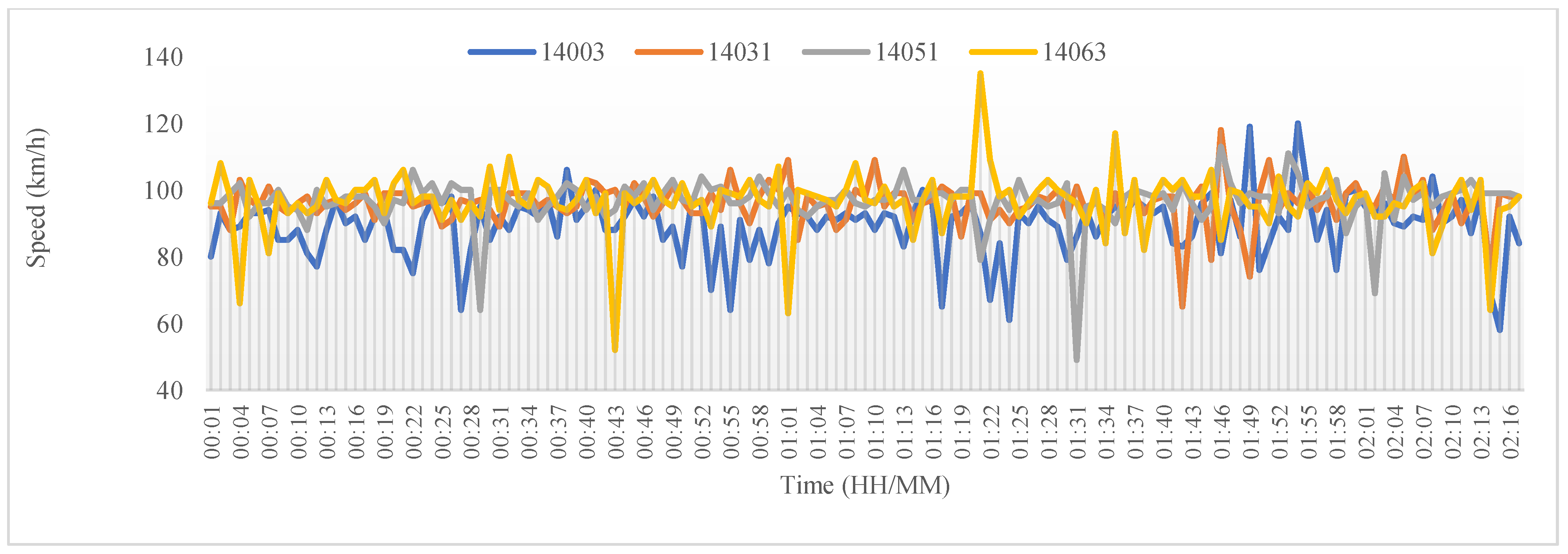
For detector 14003, the results show that LSTM provides a forecasting accuracy of 94.24% for a 5-min prediction horizon and 94.97% for a 60-min prediction horizon. For the LSTM, the accuracy does not deteriorate substantially as the prediction horizon increases, with the accuracy remaining high at 94.97% for the 60-min horizon. This shows the ability of the system to capture the complexity of longer speed prediction horizons. On the other hand, the MNN provided the least accurate predictions out of the six models tested. For detector 14031, the same trend can be noticed with accuracies not deteriorating substantially for the LSTM with longer prediction horizons. For the 10-min horizon, the accuracy is 97.55%, while it remained steady at 98.96% for the 60-min horizon. Also, it can be noted that the LSTM provides better accuracy for 10 min and 60 min prediction horizons while the GRNN, MNN and RBF outperformed the LSTM for the other prediction horizons. This may be attributed to the data patterns for detector 14031, which showed more congestion at certain times during the months of July compared with other detectors. For longer prediction horizons (45 and 60 min), the DLBP neural network had the lowest performance of 95.22% and 94.14%, respectively.
For detector 14051, the LSTM outperforms all other 6 models with an accuracy ranging from 95.61% to 99.94%. The DLBP neural network and the MNN provided the least accuracies for shorter prediction horizons up to 30 min, while the RBF had the lowest accuracy of 89.72% compared to 99.94% of the LSTM for 45 min into the future. The RNN provided the least accurate predictions for 60-min horizons with 83.16% accuracy compared to 99.43% for the LSTM.
For detector 14063, the LSTM provided a good level of accuracy for all time horizons ranging from 97.68% to 98.77%. The DLBP neural network achieved the lowest accuracy for 15, 30 and 45 min predictions compared to the six models, whereas the RBF had the lowest accuracy for 60-min horizons (91.77%) compared with the LSTM with the highest accuracy of 98.77%.
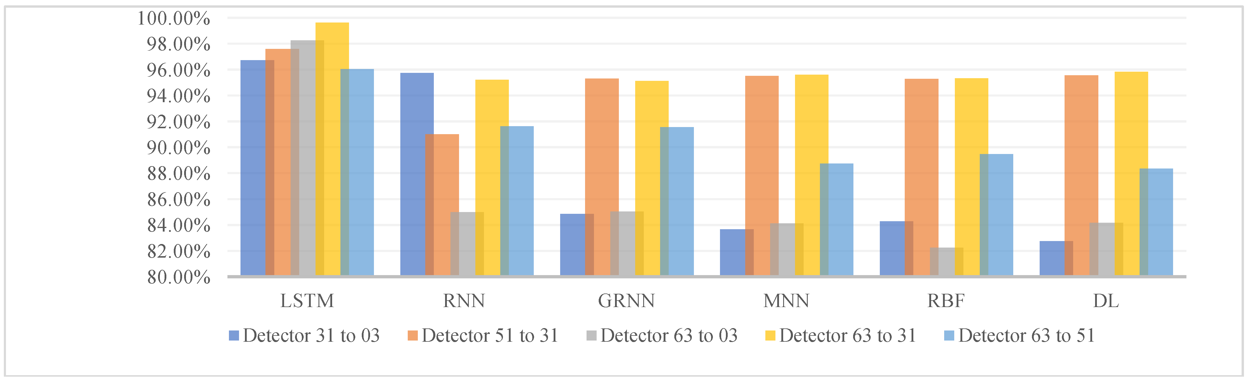
4.2.2. Westbound Direction—Spatial Prediction Accuracies
For the spatial analysis, the main observation is that the accuracy of prediction is not affected as the distance between detector locations increases (
Table 5 and
Figure 8). The LSTM provides the highest accuracy for all spatial ranges, with the accuracy ranging from 96.03% for a 5.4 km separation to 98.24% accuracy for an 18.6 km separation of detector locations. The DLBP neural network provided the lowest accuracies for short distances, while the MNN and RBF performed worse when the spatial separation increased between any two detector locations.
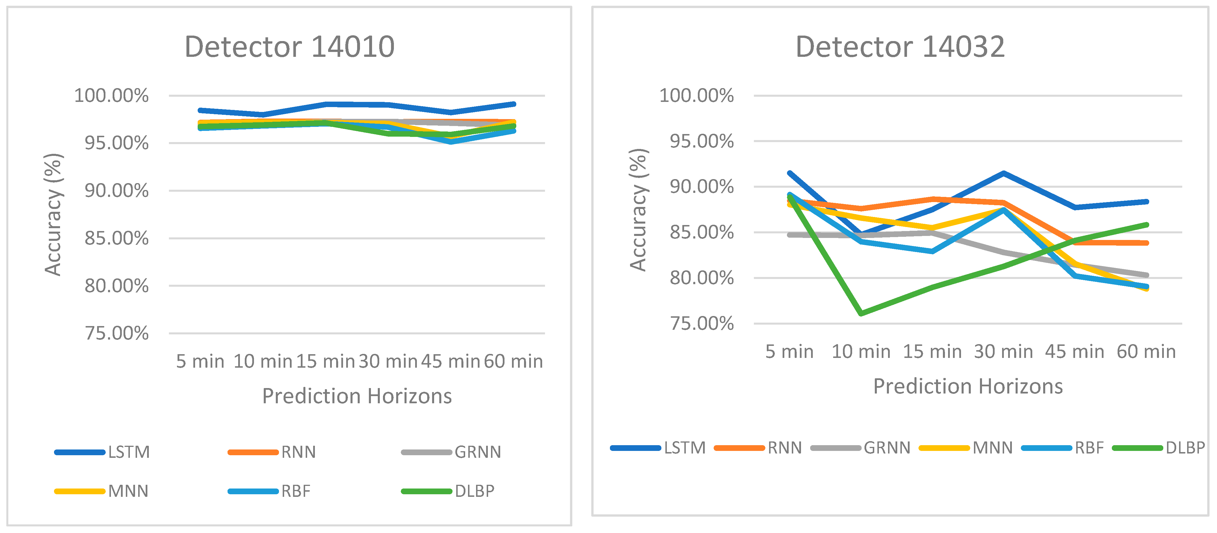
4.2.3. Eastbound Direction—Temporal Prediction Accuracies
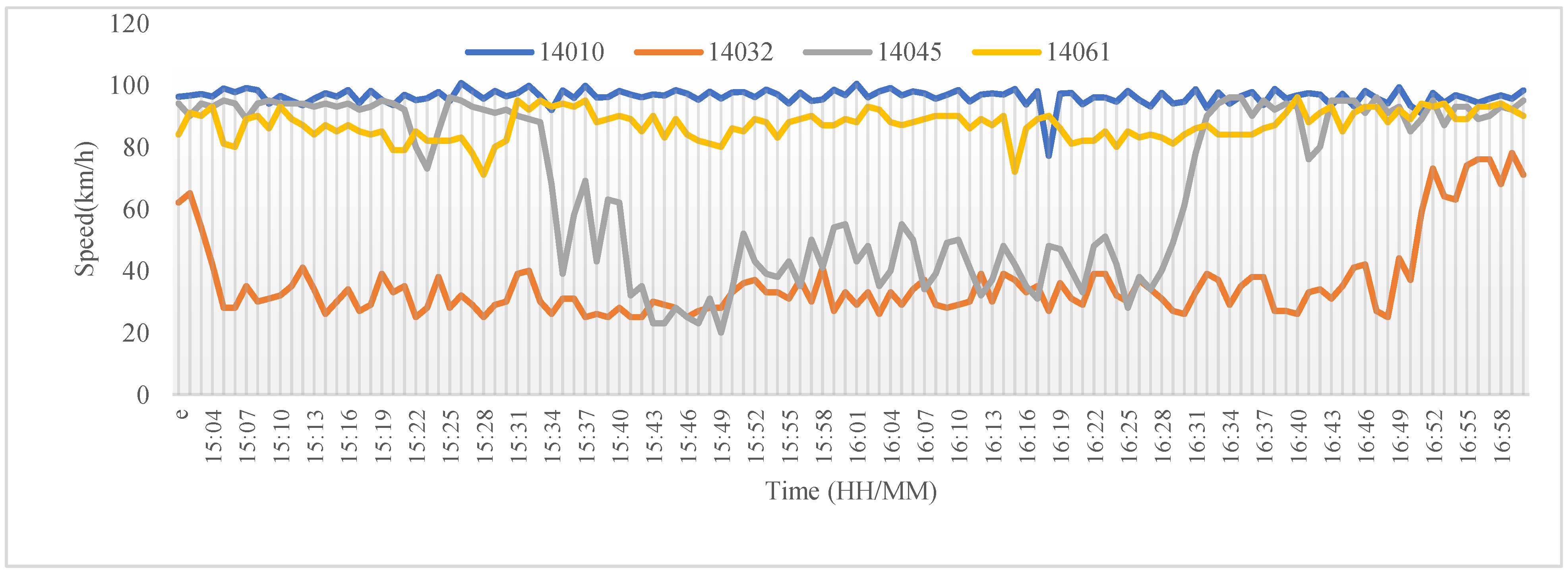
The experimental results for the temporal variations in the eastbound direction are provided in
Table 6 and
Figure 9. The cells in the table that are highlighted in orange show the highest accuracies obtained, while the cells highlighted in green show the lowest. The results show that the LSTM generally has superior performance when compared to the RNN, GRNN, MNN, RBF and DLBP neural network.
Detector 14010 shows that the LSTM provides higher prediction accuracies of 98.44% for 5-min prediction horizons and 99.10% for 60-min horizons. For the LSTM, the accuracies do not deteriorate as the prediction horizon increases. For example, the accuracy is 97.97% for the 10-min horizon and remains steady at 99.10% for 60-min prediction horizons. This shows the ability of the system to capture the complexity of a longer speed prediction horizon. For the eastbound direction, the RBF had the least accurate predictions out of the six models.
For detector 14032, the results for the LSTM were the lowest compared to all detectors from WB and EB. This is maybe due to the data patterns for this detector which experienced heavy congestion at certain times during the months of July compared to other detectors. For 10-min horizons, the accuracy is 84.74% compared to 88.37% for the 60-min horizon. Also, it can be noted that the RNN provides better accuracy for 10-min and 15-min prediction horizons. However, the LSTM provides better accuracy overall for detector 14032. For short prediction, the GRNN and the DLBP neural network provided the least accurate predictions, while for longer prediction horizons (45 and 60 min), the RBF and MNN had the lowest performance of 80.21% and 78.80%, respectively.
For detector 14045, the LSTM outperforms all other 6 models with an accuracy ranging from 96.42% to 99.01%. The DLBP neural network, MNN and RBF provided the least accuracies for shorter prediction horizons up to 30 min, while the RBF had the lowest accuracy of 93.02% compared to 96.42% for the LSTM for 45-min horizons. The GRNN provided the least accurate predictions for 60-min horizons with 91.93% accuracy compared to 98.77% and 96.05 for the LSTM and RNN, respectively.
For detector 14061, the LSTM provided good accuracy for all time horizons ranging from 96.9% to 99.95%, except for the 60-min horizon where the RBF provided the highest accuracy of 96% compared to 93% for the LSTM. For 15-min horizons, the RBF achieved the lowest accuracy of 95.93% compared to the highest accuracy of 99.80% for the LSTM.
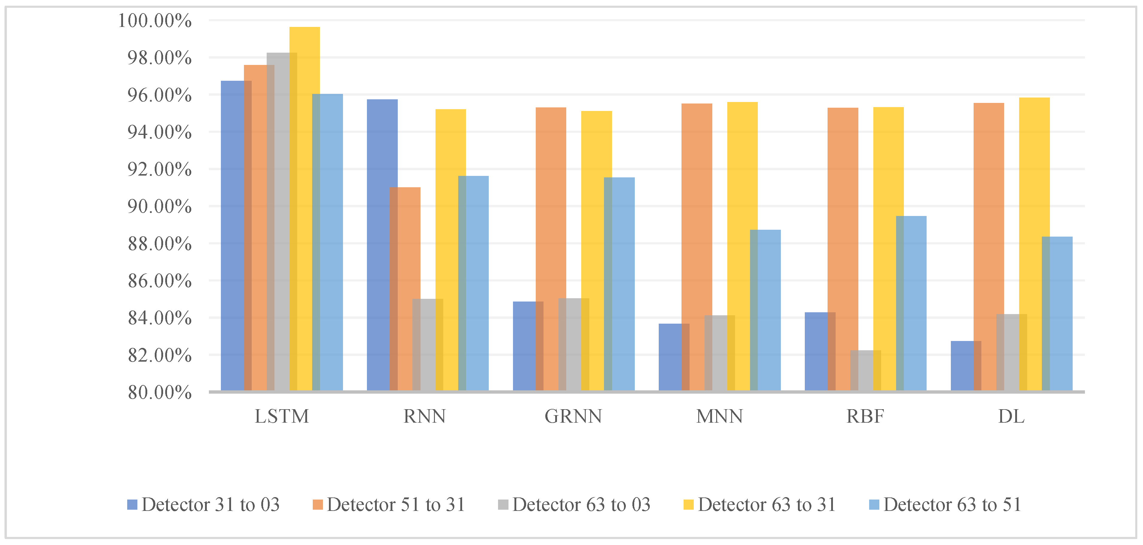
4.2.4. Eastbound Direction—Spatial Prediction Accuracies
For the eastbound direction, the results are similar for westbound reported before, where the accuracy of prediction is not affected as the distance changes. As can be seen in
Table 7 and
Figure 10, the LSTM provides the highest accuracy for most distance ranges, whereas the RNN provides the least accuracy. Overall, the LSTM provides the highest accuracy ranges for detectors that are furthest apart (15.45 km) with an accuracy result of 99.95%.


