Article

Comparing ANOVA and PowerShap Feature Selection Methods via Shapley Additive Explanations of Models of Mental Workload Built with the Theta and Alpha EEG Band Ratios

Artificial Intelligence and Cognitive Load Research Lab, Technological University Dublin, Grangegorman Lower, D07 H6K8 Dublin, Ireland
*
Author to whom correspondence should be addressed.
These authors contributed equally to this work.
BioMedInformatics 2024, 4(1), 853-876; https://doi.org/10.3390/biomedinformatics4010048
Submission received: 28 January 2024 / Revised: 6 March 2024 / Accepted: 12 March 2024 / Published: 19 March 2024
(This article belongs to the Special Issue Feature Papers in Medical Statistics and Data Science Section)

Abstract

:
Background: Creating models to differentiate self-reported mental workload perceptions is challenging and requires machine learning to identify features from EEG signals. EEG band ratios quantify human activity, but limited research on mental workload assessment exists. This study evaluates the use of theta-to-alpha and alpha-to-theta EEG band ratio features to distinguish human self-reported perceptions of mental workload. Methods: In this study, EEG data from 48 participants were analyzed while engaged in resting and task-intensive activities. Multiple mental workload indices were developed using different EEG channel clusters and band ratios. ANOVA’s F-score and PowerSHAP were used to extract the statistical features. At the same time, models were built and tested using techniques such as Logistic Regression, Gradient Boosting, and Random Forest. These models were then explained using Shapley Additive Explanations. Results: Based on the results, using PowerSHAP to select features led to improved model performance, exhibiting an accuracy exceeding 90% across three mental workload indexes. In contrast, statistical techniques for model building indicated poorer results across all mental workload indexes. Moreover, using Shapley values to evaluate feature contributions to the model output, it was noted that features rated low in importance by both ANOVA F-score and PowerSHAP measures played the most substantial role in determining the model output. Conclusions: Using models with Shapley values can reduce data complexity and improve the training of better discriminative models for perceived human mental workload. However, the outcomes can sometimes be unclear due to variations in the significance of features during the selection process and their actual impact on the model output.

1. Introduction

In many practical machine learning tasks, including interpretability [1,2], data valuation [3], feature selection [4,5], ensemble pruning [6], federated learning [7] and universal explainability [8,9], measuring the achievement of a data attribute is a central issue. Although we heavily rely on machine learning models to perform various tasks, we rarely question the validity of the decisions made by the learning algorithms used to build them. This raises legitimate questions concerning the importance of a feature during the model learning process, the value of an individual data point in a dataset during learning, which models are more valuable during an ensemble learning procedure, which vote is more important, and why. While different methods exist to address these questions, the transferable utility cooperative game approach is a more general and holistic way to tackle them, with its most popular method being based on Shapley values [10]. Cooperative game theory aims to evaluate the value of coalitions that players can form. Shapley values effectively divide a cooperative game’s overall value or payoff between its players. They assess a player’s average marginal contribution to all potential coalitions they could be a part of and are calculated by averaging their marginal contributions across all possible coalition formations. Over the years, several enhancements have been made to Shapley values, such as enhancing efficiency, symmetry and fairness [11]. When considering machine learning and corporate game theory, each feature is treated as a player in a game, and the Shapley value of a feature represents its contribution to the model’s overall prediction accuracy. To calculate Shapley values, one must consider all possible feature subsets and compute each feature’s marginal contribution to the prediction accuracy. Although this process can be computationally intensive, recent algorithm and computing power advancements have made it viable for larger and more complex datasets.
Shapley values are widely used in machine learning to explain how individual features or variables contribute to a model’s final prediction. Each feature is assigned a numerical value representing its impact on the output, resulting in a clear and understandable explanation of the model’s behaviour. This information is invaluable for identifying critical features, improving model performance, and building trust and accountability in machine learning models [1,12,13]. Using Shapley values in machine learning offers a significant advantage as they support an unbiased way of interpreting the behaviour of various learnt models [14]. Additionally, Shapley values can be utilized to explain the predictions of black-box models, which are typically challenging to interpret using other methods [15]. Some examples of how Shapley values are applied in machine learning include:
  • Feature selection: Identifying the most significant features and eliminating any irrelevant or redundant ones is crucial for creating precise and efficient models, especially in datasets with numerous dimensions [5,16].
  • Model comparison: Comparing the performance of various models and pinpointing their strengths and weaknesses can aid in selecting the most suitable model for a particular task and identifying areas for enhancement [17].
  • Bias detection: Identify any potential features that may result in bias or discrimination in the model’s predictions. It is imperative to take immediate action to address this bias and improve the model’s fairness [9].
  • Explainable AI: It is important to clearly and unequivocally explain how the model behaves to establish trust and accountability in automated decision-making systems [1,8,18].
Calculating Shapley values for extensive datasets is computationally expensive, rendering its use in practical situations difficult. Studies have examined these difficulties and drawbacks in machine learning [19,20]. Moreover, understanding and interpreting Shapley values can be subjective and influenced by the selection of the model’s starting point, potentially affecting the outcomes [1,21]. Algorithm design and computing power have recently made significant progress, broadening their applications and creating new research opportunities in this field. Shapley values can serve as a useful tool for evaluating intricate classification models. For instance, they can be applied to the models for distinguishing between the self-reported perceptions of mental workload via electroencephalographic activity. Research has shown that EEG band ratios, particularly those in the theta and alpha bands, are linked to various mental workload states [22,23]. Studies support the idea that these measures could be used as indicators of workload [24,25], and as a result, they could be incorporated into various machine-learned models to discriminate the self-reported perceptions of mental workload [26]. There have been numerous proposals for machine learning models aiming to distinguish the self-reported perceptions of mental workload [25,26,27,28]. However, mental workload research using EEG data in the area of model explainability with the use of Shapley values is currently limited.
This paper investigates the impact of Shapley-based feature selection methods in comparison to statistical feature selection methods on the capability of machine learning models to distinguish the self-reported perceptions of mental workload using alpha-to-theta and theta-to-alpha ratios extracted from EEG data. The formulated research question is: What is the difference in performance between these two methods? The innovative aspect of the paper resides in the fact that, by integrating explainability in feature selection methods, it is possible to unveil a potential new dimension for understanding the complex relationship between EEG band ratios and self-reported mental workload levels. This innovation would empower the machine learning models to make accurate predictions and provide invaluable insights into the specific EEG features that drive these predictions to human stakeholders. As a result, this might enhance the transparency and interpretability of these models, enabling researchers and clinicians to decipher the intricate neurological processes underpinning mental workload variations with a higher level of precision and clarity than existing research works. With the fusion of feature selection methods and model explainability with EEG band ratio data, it is possible to introduce a potential research path in comprehending cognitive states, paving the way for more targeted interventions, data-driven discoveries, and a deeper comprehension of mental workload dynamics. This paper is a step towards that direction.
The remainder of this paper is organised as follows: Section 2 provides the background concepts on alpha-to-theta and theta-to-alpha EEG band ratios as well as statistical and Shapley-based feature extraction on EEG data; Section 3 outlines the experiment design for feature extraction from EEG band-ratios using Shapley values and its comparison with the traditional statistical ANOVA method; Section 4 presents the result, while Section 5 critically discusses them. Eventually, Section 6 highlights the contribution to the body of knowledge and presents future directions of research.

2. Related Work

This section will thoroughly define Shapley values and examine their significant impact on machine learning. Furthermore, mental workload and its assessment methods will be precisely defined. Lastly, statistical and Shapley-based feature selection methods will be exhaustively explored.

2.1. Shapley Values in Machine Learning

To accurately define the Shapley values in collaborative game theory, it is crucial to have a thorough grasp of the fundamental formalisms and definitions involved. The definitions provided below are important in that regard [6,10].
Player sets and coalitions: Let us consider the machine learning features as being players in a cooperative game provided by a finite set: F = { 1 , 2 , 3 , , n } . We denote a non-empty subset N F as a coalition and F as grand coalition.
Cooperative game: A cooperative game between features is represented by the pair ( F , υ ) . Here, υ : 2 F is a coalition function that assigns a real value to each feature coalition. It is worth noting that υ ( ) = 0 is also necessary to consider the function a collaborative game.
Feasible pay-off vector sets: In a cooperative game ( F , υ ) , the set of feasible payoff vectors is defined as Z ( F , υ ) , which consists of all vectors z F that satisfy the condition i F z i υ ( F ) .
Solution concepts and vectors: When dealing with collaborative games, a solution concept Φ is a way of mapping a subset Φ ( F , υ ) Z ( ( F , υ ) ) to a specific game ( F , υ ) . In order for a solution vector ϕ ( F , υ ) F to be considered a solution to the cooperative game ( F , υ ) , it must satisfy the solution concept Φ , meaning that ϕ ( F , υ ) Φ ( F , υ ) . A single-valued solution concept would exist if, for every ( F , υ ) , the set Φ ( F , υ ) only contains one element.
Feature set permutations: We can refer to the set of all permutations on a given set F as Π ( F ) . Within this set, there exists a specific subset of permutations represented by π Π ( F ) , where π i denotes the position of feature i within the permutation π .
The predecessor set: of a feature i F in a permutation π is a coalition of the form: P i π = { j F | π j < π i } .
Assuming the given permutation of three features is π = ( 3 , 2 , 1 ) , the predecessor set for this permutation would be: P 1 π = ( 3 , 2 ) for the first feature, P 2 π = ( 3 ) for the second feature, and P 3 π = for the third feature.
Given these definitions, we can now define the Shapley values as:
ϕ i s = 1 Π ( F ) π Π ( F ) [ υ ( P i π { i } ) υ ( P i π ) ]
where the expression inside the sum represents the ith features marginal contribution within permutation π . According to the equation, the Shapley value for a feature is the average marginal contribution of that feature to the predecessor set’s value, calculated across all possible permutations of the feature set.

2.2. The Concept of Mental Workload

Mental workload is crucial for studying human performance and is applied in various fields, such as medicine [29], education [30], web-design [31], and transportation [32], among others. The concept of mental workload is complex and has multiple levels, which can be difficult to define. It is often confused with cognitive effort [33], leading to ambiguities in its definition. This multifaceted complexity makes it challenging to understand the concept entirely. There are numerous interpretations of mental workload, as stated in the research by Hancock [34]. However, a recent comprehensive definition incorporating various perspectives is that Mental Workload (MWL) reflects the level of engagement of a limited pool of resources during the cognitive processing of a primary task over time. This is influenced by both external stochastic environmental and situational factors, as well as the internal characteristics of the human operator, and it is necessary for managing static task demands through dedicated effort and attention [35]. Based on the Multiple Resource Theory (MRT), this definition states that resources have a limited capacity and using multiple resources simultaneously can lead to reduced performance and increased mental workload. The theory suggests that resource selection and allocation depend on task demands, individual differences and context. To optimize the use of multiple resources, task design and training can minimize the mental workload and improve resource allocation and coordination, as outlined in Wickens’ work on the subject.
Numerous techniques are utilized to measure mental workload [34]. One method uses subjective measures, which involves collecting feedback from individuals who have interacted with a task and system. This feedback is typically obtained through post-task surveys or questionnaires. Some common subjective measurement approaches are the NASA Task Load Index (NASATLX), the Workload profile (WP), and the Subjective Workload Assessment Technique (SWAT). Another method is task performance measures, which includes primary and secondary task measures. This method objectively measures an individual’s performance related to a task. Examples of such measures include the time completion of a task, reaction time to secondary tasks, number of errors on the primary task and tracking and analyzing different actions performed by a user during a primary task. Lastly, physiological measures are based on analyzing the physiological responses of the human body. Examples of such measures include EEG (electroencephalogram), MEG (magnetoencephalogram), Brain Metabolism, Endogenous Eye blinks, Pupil diameter, heart rate measures, or electrodermal responses.
“EEG band ratios” refer to comparing power or amplitude between two frequency bands present in an electroencephalographic (EEG) signal. These ratios are widely utilized in neuroscience research to study brain activity during various states, including sleep, attention, alertness, emotion, and mental workload. In particular, the alpha and theta bands are frequently studied in the context of mental workload due to research indicating a correlation between these bands and increased mental workload. Specifically, an increase in the theta power band in the frontal brain region and a decrease in the alpha power in the parietal region is associated with increased mental workload [36]. Measuring mental workload through EEG band ratios and correlating objective brain activity (alpha-to-theta and theta-to-alpha) with the subjective self-reports of workload is difficult due to the disparity between the measures. It is crucial to investigate the convergence of measures between objective brain activity and the self-reported perception of mental workload [37]. Eventually, various analytical models of cognitive load have been built, with inductive and deductive techniques [35]. For example, Machine Learning has been used in conjunction with EEG data to inductively model cognitive load in a self-supervised way, without human intervention in selecting features [38]. Similarly, mental workload is represented and assessed via defeasible reasoning as a non-monotonic knowledge-representation technique that allows one to embed the deductive knowledge of a human reasoner together in a model [39,40].

2.3. Feature Selection with Statistical and Shapley-Based Methods

Various inductive data-driven techniques have been employed in mental workload modeling. However, one of the challenges is to create a group of independent features that can be mapped inductively to a target feature, which is typically a person’s subjective perception of workload or a physiological measure of bodily activation. In Machine Learning, various methods are available to automatically select the most pertinent, descriptive and distinguishing features from a larger set of features for solving classification or regression tasks. These techniques are briefly described in the following sub-section.

2.3.1. Traditional Statistical Feature Selection Methods

Feature selection methods in statistics help pick out the most significant features from a large pool of available features. This process reduces the data’s complexity while retaining as much important information as possible. A preferred approach is the mutual information-based feature selection, which assesses the dependence between the features and the target variable [41]. The mutual information score assesses the significance of features and chooses the most important K features. It is an effective and efficient method for both categorical and continuous variables. Another widely used method for selecting statistical features is the chi-square test. It determines the relationship between categorical variables and chooses the features that are most likely to be related to the target variable. This test calculates the chi-square statistic for each feature and sorts them based on their p-values. The features with lower p-values are more significant to the target variable. This method is effective in selecting features that are highly correlated with the target variable [42]. Another statistical method for feature selection is the ANOVA F-test. It is specifically used for choosing features with continuous variables and calculates the disparity between the means of the variables for the distinct categories of the target variable [43]. The ANOVA F-test evaluates features by their F-statistic or F-score. This ratio measures the difference in variance between groups and within groups. Features with a high F-statistic or F-score significantly impact the target variable when chosen. This method is effective for non-skewed data.

2.3.2. Shapley Values and Their Application as a Feature Selection Method

In the Shapley-based feature selection method, machine learning model input features are treated as players, while the model’s performance is considered the payoff. The Shapley values quantify the contribution of each feature to the model’s performance on a given set of data points [44]. The features can be ranked, selected, or removed based on these values. To define the Shapley values in machine learning, we consider the feature set F = { 1 , , n } and S F . We also define the train and test feature vector sets as X S t r a i n = { x i t r a i n | i S } and X S t e s t = { x i t e s t | i S } . We use f s ( · ) to represent a machine learning model trained using X S t r a i n as input. The payoff is υ ( S ) ) = g ( y , y ^ S ) , where g ( · ) is a goodness of fit function, y is the ground truth, and y S = f S ( X S t e s t ) is the predicted target. The Shapley values were widely used as a feature selection method across various contexts and applications [16,45]. It is important to note that both the ANOVA F-score and Shapley-based feature selection methods have been utilized to analyze EEG data. These selection methods have been applied and compared in various situations, such as the diagnosis of Parkinson’s disease [46], recognizing emotions [47], detecting sleep apnea and depression [48,49], and diagnosing schizophrenia [50]. Although there is a considerable amount of research comparing the ANOVA F-score and Shapley-based feature selection methods in different problem scenarios, there is limited research on comparing these feature selection methods for measuring the mental workload physiologically using EEG band ratios. Considering the highly subjective nature of assessing mental workload conditions using machine learning, explaining the relevance of these features is of the utmost importance. In this regard, limited work is seen, for example, on brain state classification using EEG [51] or the cross-sectional classification of mental workload using eye tracking features [52].

3. Materials and Methods

To tackle the research question laid out in Section 1, a research hypothesis has been developed:
Hypothesis 1. 
IF high-level EEG features are selected using the Shapley-value-based method. Then, the resulting machine learning model will demonstrate higher performance in discriminating the self-reported perceptions of mental workload compared to models that use statistical feature selection methods.
This study follows the processing pipeline presented in [25], but with some modifications in the subsequent sections. The research hypotheses were tested through comparative empirical research, and more details can be found in Figure 1 and the following subsections.

3.1. Dataset

The STEW (Simultaneous Task EEG Workload) dataset was selected for an experiment. This dataset consists of raw EEG data collected from 48 subjects through 14 channels [53]. Two experimental conditions were studied: the rest state and a multitasking cognitive processing speed test called SIMKAP. The Emotiv EPOC EEG headset was used to record the data, with a sampling frequency of 128 Hz. The recordings included 19,200 data samples across the 14 channels. After each task, the subjects rated their perceived mental workload on a scale of 1–9, which was used to determine whether there was an increase in cognitive load during the SIMKAP test compared to the rest state.

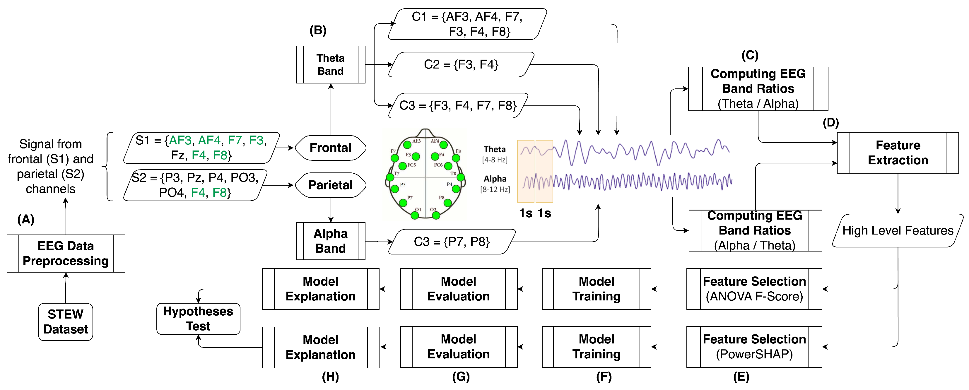
3.2. EEG Data Pre-Processing

Before analyzing the raw EEG data, removing noise through a denoising pipeline is important. This process is illustrated in point (A) of Figure 1 and follows Makoto’s pre-processing pipeline [54]. The pipeline involves re-referencing channel data to average reference, high-pass filtering each channel at 1 Hz, and using Independent Component Analysis (ICA) for artefact removal. ICA separates the EEG signal sources into 14 independent components for each subject. To remove artefacts, 14 components are generated and it is checked whether the values are outside the “z-score±3” range [55], which are then considered artefacts and set to zero. The remaining “good” components are converted back to the original neural EEG signal using inverse ICA.

3.3. Computing EEG Band Ratios from the Theta and Alpha Bands as Indicators of Objective Mental Workload

The study utilized a baseline of frontal and parietal electrodes based on the 10–20 international system. These were cross-referenced with electrode availability from the Emotiv EPOC EEG headset. Due to the limited availability of electrodes, three frontal and one parietal cluster were created using specific combinations of electrodes and channel aggregation approaches. The channel clusters are depicted in Table 1 and marked as point (B) in Figure 1.
The rationale for using the three selections from the theta band ( c 1 θ , c 2 θ , and c 3 θ ) was to use the symmetrical and iterative enlargement of the electrode numbers on the frontal brain region to provide better coverage. We utilized the average power spectral density (PSD) values from the alpha band in cluster c α , and the average PSD values from the theta band in clusters c 1 θ , c 2 θ , and c 3 θ [23] to calculate the alpha-to-theta and theta-to-alpha ratios. We strategically selected different clusters from frontal and parietal electrodes, as depicted in Table 1 and point (C) in Figure 1, to acquire three alpha-to-theta and three theta-to-alpha ratios, resulting in six mental workload indexes. These indexes were then utilized for feature extraction, selection, and model training. Henceforth, we will refer to these indexes as our mental workload indexes given in Equation (2)
M W L i n d e x e s { a t 1 , a t 2 , a t 3 , t a 1 , t a 2 , t a 3 }
where: a t 1 = c α c 1 θ , a t 2 = c α c 2 θ , a t 3 = c α c 3 θ , t a 1 = c 1 θ c α , t a 2 = c 2 θ c α and t a 3 = c 3 θ c α

3.4. Feature Selection Using Statistical and Shapley-Based Methods

The rationale behind selecting statistical and Shapley-based feature selection methods for our study lies in their efficiency and easy interpretability. Table 2 outlines the comparison of feature selection methods outlined in our study against four other methods (Recursive Feature Elimination (RFE), Least Absolute Shrinkage, and Selection Operator (LASSO), Random Forest Feature Importance and Principal Component Analysis (PCA)) in terms of interpretability, assumptions, scalability, robustness, and performance.
From the aforementioned table, the research strength assumptions of the study can be summarized around the following points:
  • By applying the statistical (ANOVA F-score) and Shapley-based (PowerSHAP) methods, the research tends to demonstrate a comprehensive approach to feature selection, closely matching the type of data we explore (EEG) and model complexities that arise from it, thus providing a methodological diversity to the study.
  • Whilst Shapley-based feature selection and model interpretability may vary, including ANOVA F-score ensures that at least one method in the study provides straightforward interpretability, which is expected to enhance the comprehensibility of the findings.
  • The study also tends to benefit from the robustness to outliers and nonlinear relationships of Shapley-based feature selection methods, while still leveraging the efficiency and performance of ANOVA F-score in identifying significant feature differences.
  • Comparing Shapley-based feature selection methods with other common feature selection techniques, the research aims to showcase a broad understanding of the importance of feature selection in Mental Workload Studies using EEG, offering insights into the strengths and limitations of various feature selection approaches in the context of model explainability.

3.4.1. Statistical Feature Selection Methods

It is important to extract high-level features from MWL indexes to discover unique properties that may not be detectable by solely considering the indexes. Time Series Feature Extraction Library (TSFEL) (https://tsfel.readthedocs.io/en/latest/index.html accessed on 15 December 2023) is a tool that can extract high-level features from the MWL indexes described in Equation (2). TSFEL provides a variety of statistical properties that can be extracted from different types of data, including frequency and temporal data, and presented as point (D) in Figure 1. Initially, a large number of features are taken into consideration, and feature reduction is performed using statistical and Shapley-based feature selection methods, as explained in Section 2.3.1 and illustrated as point (E) in Figure 1. The “SelectKBest” feature selection algorithm is used for statistical feature selection, which ranks features based on the ANOVA F-score between a feature vector and a class label. Through an iterative process of supervised model performance evaluation [25], the optimal number of retained features is determined to be seven.

3.4.2. Shapley-Value-Based Feature Selection Methods
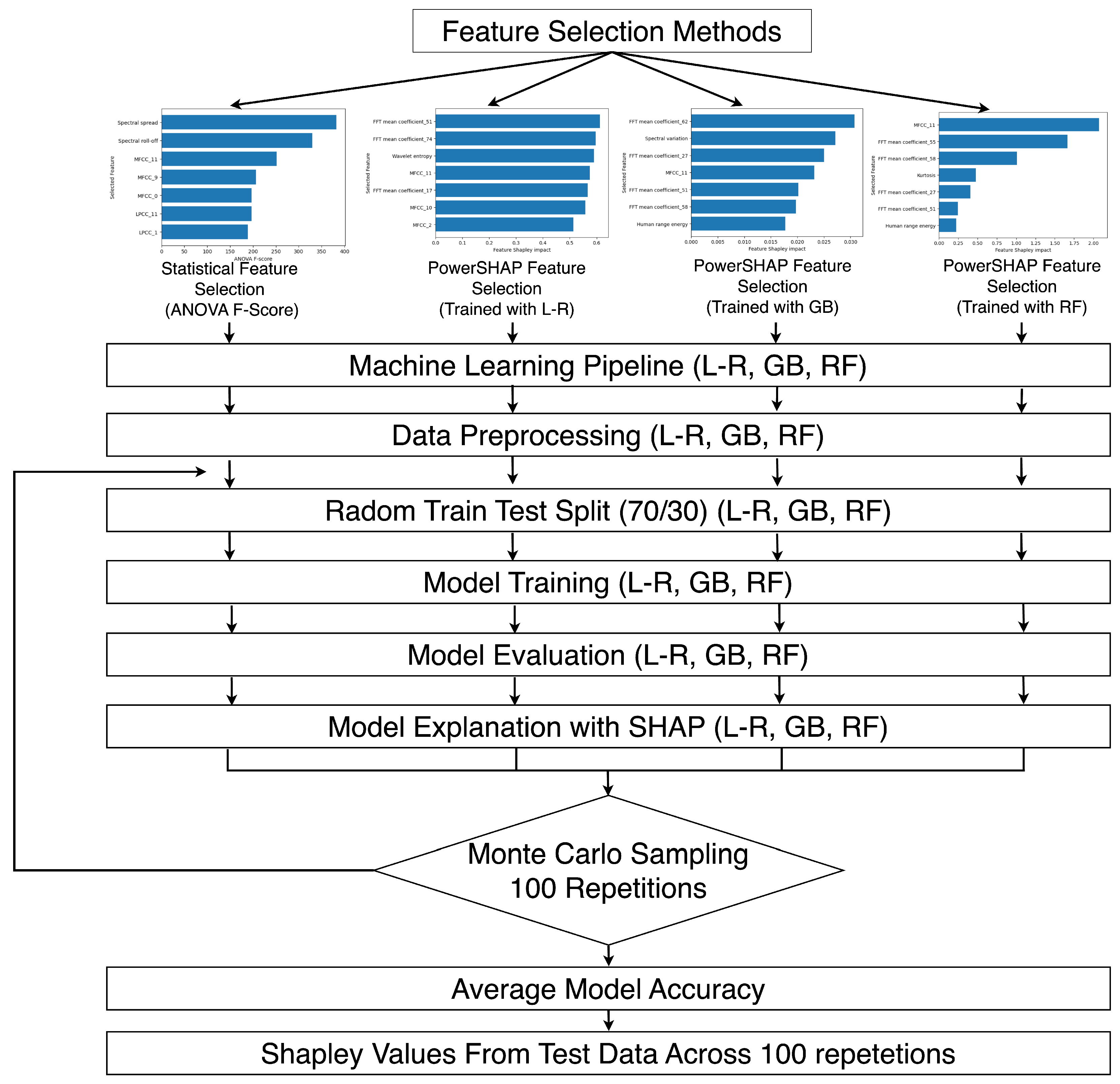
The Shapley-based feature selection method utilizes the “Powershap” algorithm [56]. Powershap is designed to identify features that have a greater impact on predictions than random features. The algorithm comprises the Explain and the Core Powershap components. In the Explain component, multiple models are created using different random features, and the average effect of all features is explained using Shapley values. In the Core Powershap component, the effects of the original features are statistically compared to the random feature, allowing for the selection of more informative features.
To evaluate the correlation and minimize multicollinearity, attention is given to the Pearson correlation between features selected with both the ANOVA F-score and PowerSHAP. Multicollinearity reduction is critical to maintaining the predictive power of each feature. Highly correlated features can negatively impact the model and not contribute to further training. Therefore, a correlation threshold of ± 0.5 is recommended for optimal model performance [57].

3.5. Model Training

The modeling and training process aims to develop classification models that can differentiate self-reported mental workload scores from independent features selected using statistical (SelectKBest with ANOVA-F score) and Shapley-based (Powershap) selection methods. This is illustrated under point (F) in Figure 1. Instead of task load conditions, mental workload self-assessment scores are selected as the target feature because they provide a more reliable indicator of user experience. Different task load conditions can result in varying levels of cognitive load, and mental workload can be influenced by factors such as prior knowledge, motivation, time of day, fatigue, and stress [34]. The target feature range is divided into two levels of mental workload, “suboptimal MWL” and “super optimal MWL”, based on the parabolic relationship between mental workload and performance [30]. Scores ranging from 1 to 4 were grouped as “suboptimal MWL” while scores from 6 to 9 were categorized as “super optimal MWL”. Scores of 5, indicating a neutral mental workload experience, were disregarded as they could potentially complicate the distinction between “suboptimal/super optimal”. This approach simplified the model training into a binary classification problem. In this study, we utilized three techniques for learning classification models: Logistic Regression (L-R), Gradient Boosting (GB), and Random Forest (RF), which have been previously used in research involving longer EEG recordings [58]. Logistic regression and Gradient Boosting are error-based methods and are well suited for binary classification tasks, which is the focus of our study. On the other hand, Random Forest is an information-based ensemble learning technique that can identify important features by calculating their information gains during model training across multiple decision trees. We utilized separate training processes to train each classification model. These training processes involved selecting features using statistical methods like SelectKBest with ANOVA-F score and Shapley-based methods like PowerSHAP. Since our study used a small dataset of only 48 subjects, we employed a repeated Monte Carlo sampling for model training and validation, following this order:
  • For model training, a randomised 70% of subjects are chosen from both the “suboptimal MWL” and “super optimal MWL” categories, which are dependent features.
  • The remaining 30% of the data is reserved for model testing.
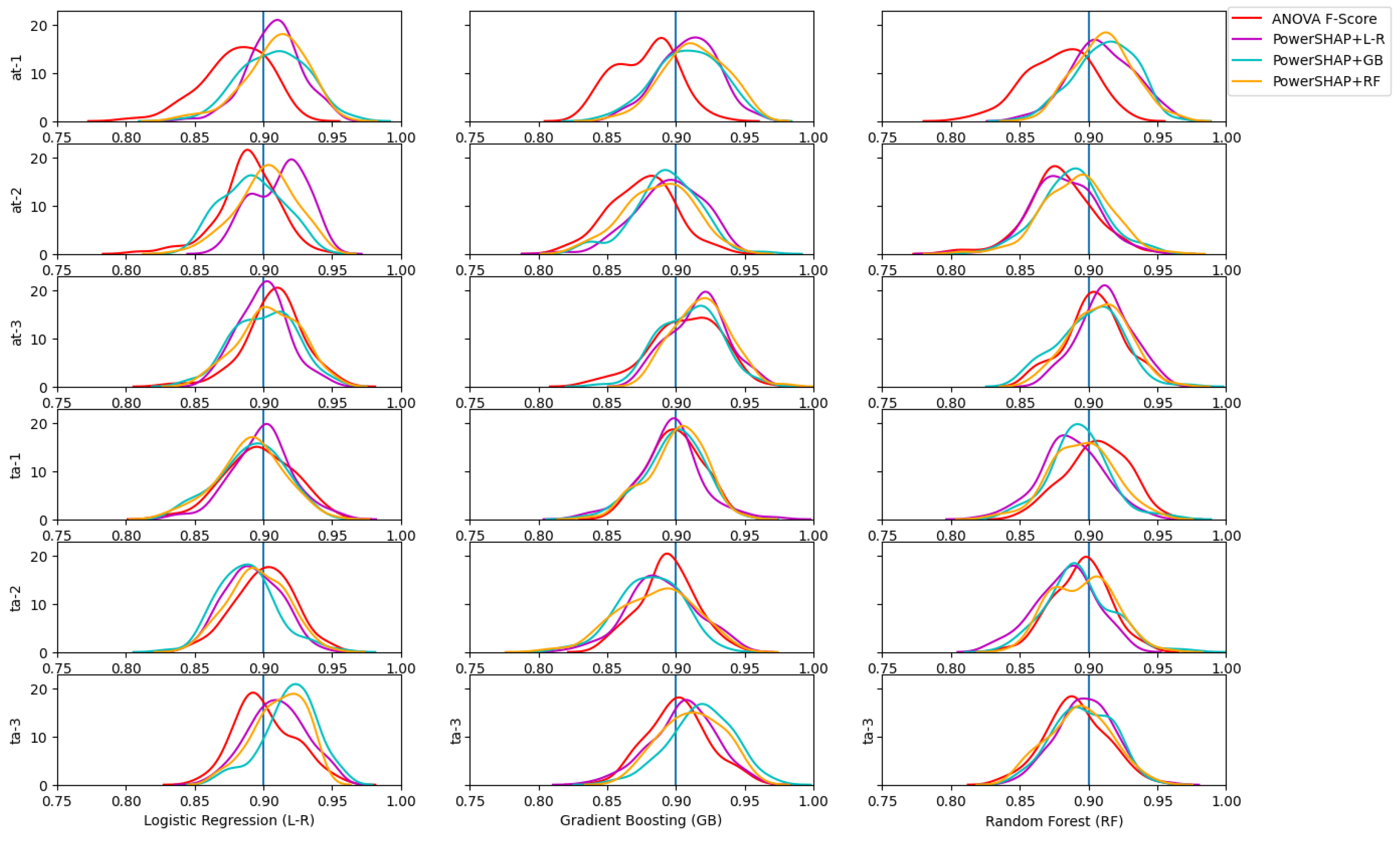
  • To capture the probability density of the target variable, the above splits are repeated 100 times to observe random training data.
To ensure the validity and robustness of the comparisons between different models and techniques a separated training, evaluation and explanation runs is performed for every Monte Carlo run. Figure 2 illustrates this process.
From the figure, it can bee seen that, for each feature selection methods, we put the selected features separately to the machine learning pipeline consisted of the steps such as: data preprocessing by scaling the data using the standard scaling method; a random 70/30 train test split across 100 iterations; model evaluation with accuracy, recall, precision and f1-score measurements and model explanation for each iteration during Monte Carlo sampling process. Finally, an averaging accuracy across 100 iterations represents the final model accuracy. The Shapley values across 100 repetitions are used to interpret the feature contributions to the model output for each of the machine learning techniques utilized (L-R, GB, and RF).
To overcome the issue of a small dataset, we implemented a synthetic data generation strategy using deep learning with GANs (Generative Adversarial Networks) [59]. We ensured the quality of the synthetic data was similar to that of the original training set by analyzing a synthetic quality score metric. This scoring metric assessed the Field Correlation Stability, Deep Structure Stability, and Field Distribution Stability [25] to provide an overall quality score. We used the same training process for the original and combined (original + synthetic) data with the same Monte Carlo sampling. To train the models, we randomly selected 70% of the subjects and used the remaining 30% for testing, with 100 iterations. During model training, we utilized Z-score normalization to minimize the mean and maximize the standard deviation. This approach allowed us to transform extreme values in the dataset into values that were no longer significant outliers, thus reducing their impact.

3.6. Model Explainability and Evaluation

The SHAP method is used to explain the model’s output. This method attributes the importance of each feature to the model’s predictions through Shapley values. SHAP calculates the contribution of each feature by considering all possible feature combinations and comparing the predictions with and without that feature. Considering their interactions allows for a more accurate attribution of importance to each feature. The SHAP values can be visualized through various SHAP plots, which depict the contribution of each feature to the model’s predictions for a specific instance. Usually, these plots show features that either increase or decrease the target value. Overall, SHAP helps to interpret a machine learning model’s output by explaining each feature’s importance to the predictions. This can be useful in understanding the model’s behavior and identifying areas for improvement. This research study uses evaluation metrics to measure how well-trained models perform when faced with new data. The metrics used include True Positives (tp), True Negatives (tn), False Positives (fp), and False Negatives (fn). These metrics calculate the model’s accuracy, precision, recall, and f1-score. Using these metrics, the researchers can assess how well the models can distinguish the self-reported perceptions of mental workload. The best model minimizes either fp or tn, but this comes at a cost to the other metric. In this sense, the f1-score is also useful as it considers both precision and recall since it represents the harmonic mean between them. The evaluation of the model performance using these metrics was applied to the SelectKbest algorithm with the ANOVA-F score and Shapley-based feature selection methods using PowerSHAP with Logistic Regression (L-R), Gradient Boosting (GB), and Random Forest (RF).

4. Results

4.1. EEG Artifact Removal

For every one of the 48 subjects, both the “Rest” and “Simkap” task load conditions have their raw EEG signal undergo artefact removal separately. On average, between one and two ICA components are removed from the EEG data for both conditions according to the methodology outlined in [25,55]. These components are zeroed out, and the EEG multi-channel data are reconstructed through inverse ICA. Since most subjects had at least one bad component removed, it is reasonable to assume that some artefact was eliminated from the EEG signal, allowing for further computations of the alpha and theta bands [60].

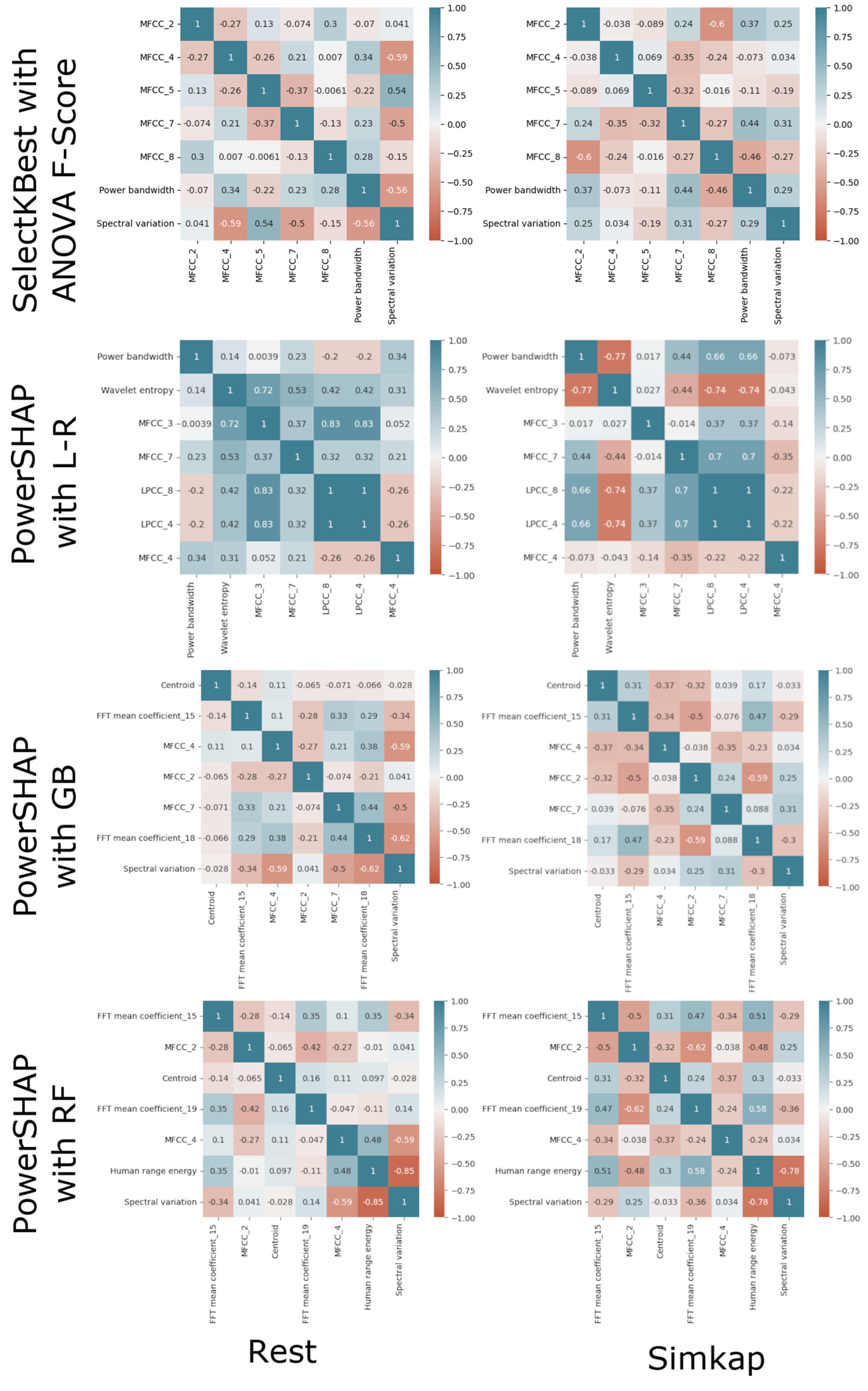
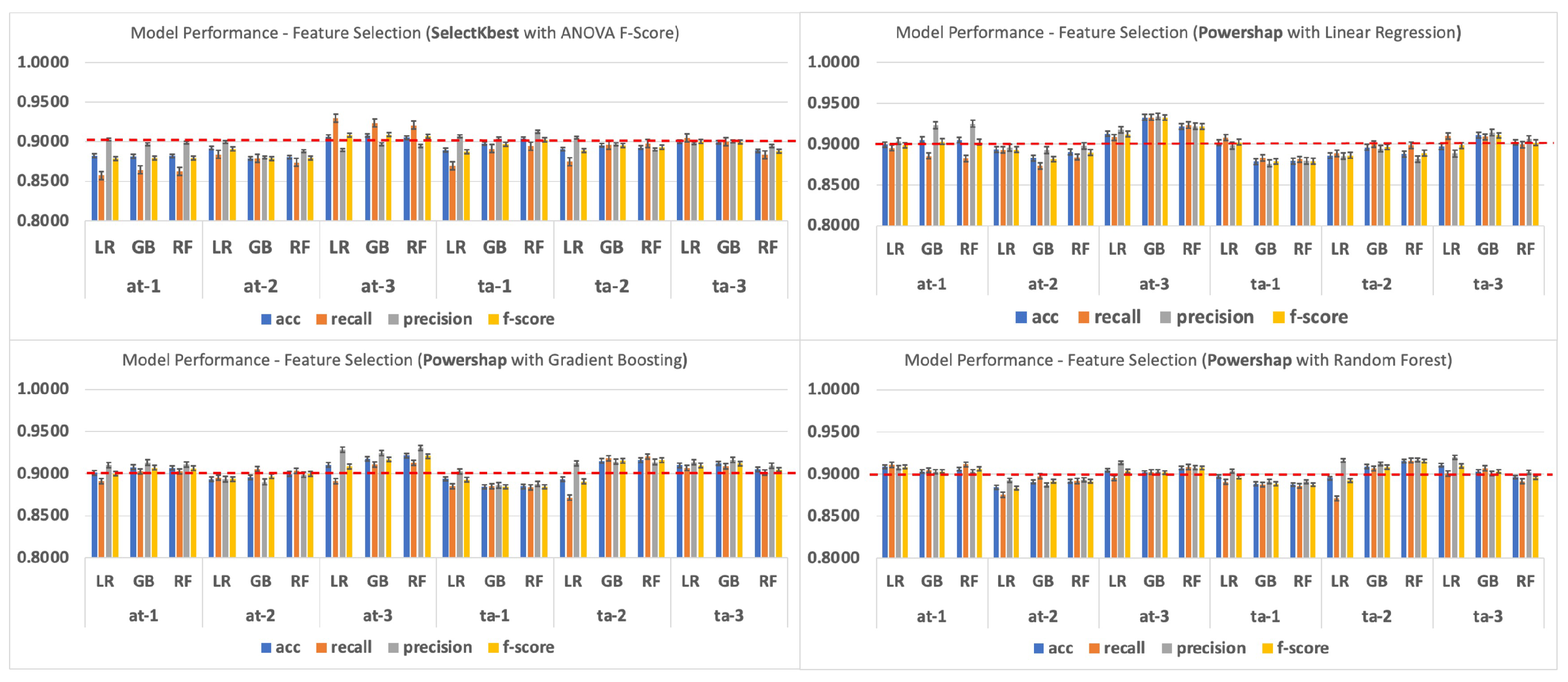
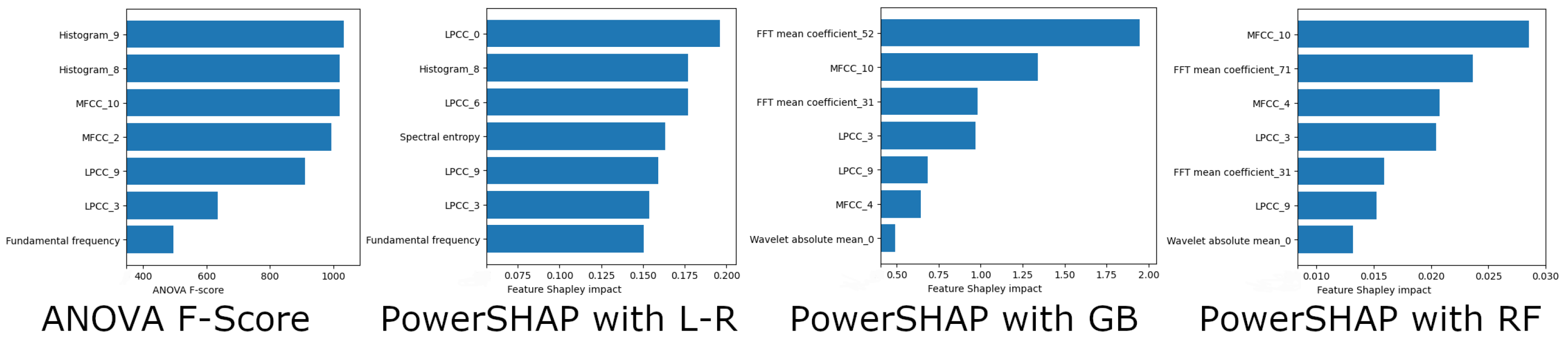
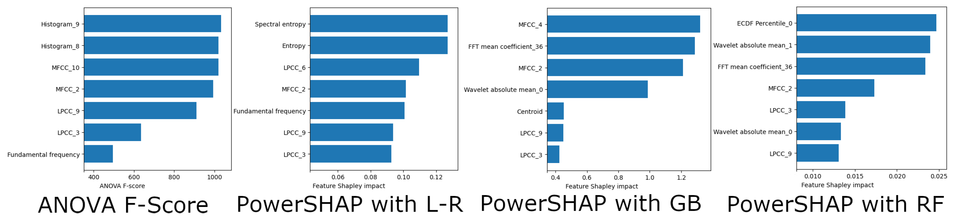
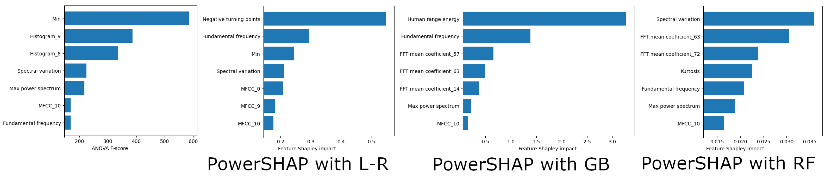
4.2. Evaluation of Feature Selection

TSFEL extracted 210 (the complete list of features can be found in https://www.frontiersin.org/articles/10.3389/fninf.2022.861967/full#supplementary-material (accessed on 15 December 2023)) high-level features from the objective mental workload indexes across the frequency and temporal domains. ANOVA F-score and PowerSHAP impact values are calculated for each feature, and the ones with the highest values are kept for model training. To use the SelectKBest algorithm, an initial number of features is required, as mentioned in the design Section 3.4.1.
Therefore, we use an iterative approach to gradually include features during model training and evaluate the model’s accuracy at each iteration. This process of optimal feature selection is performed on data from the original dataset, identifying seven optimal features as displayed in Figure 3 [25]. As a result, we retain the seven highest-ranked features with the highest ANOVA F-score values from SelectKbest and the seven highest feature impact from Shapley values retrieved from PowerSHAP with Logistic Regression (L-R), Gradient Boosting (GB), and Random Forest (RF) for the training process. Additionally, Pearson correlation among features shows a mild correlation between features as depicted in Figure 3, as grouped by task conditions (“Rest” and “Simkap”).

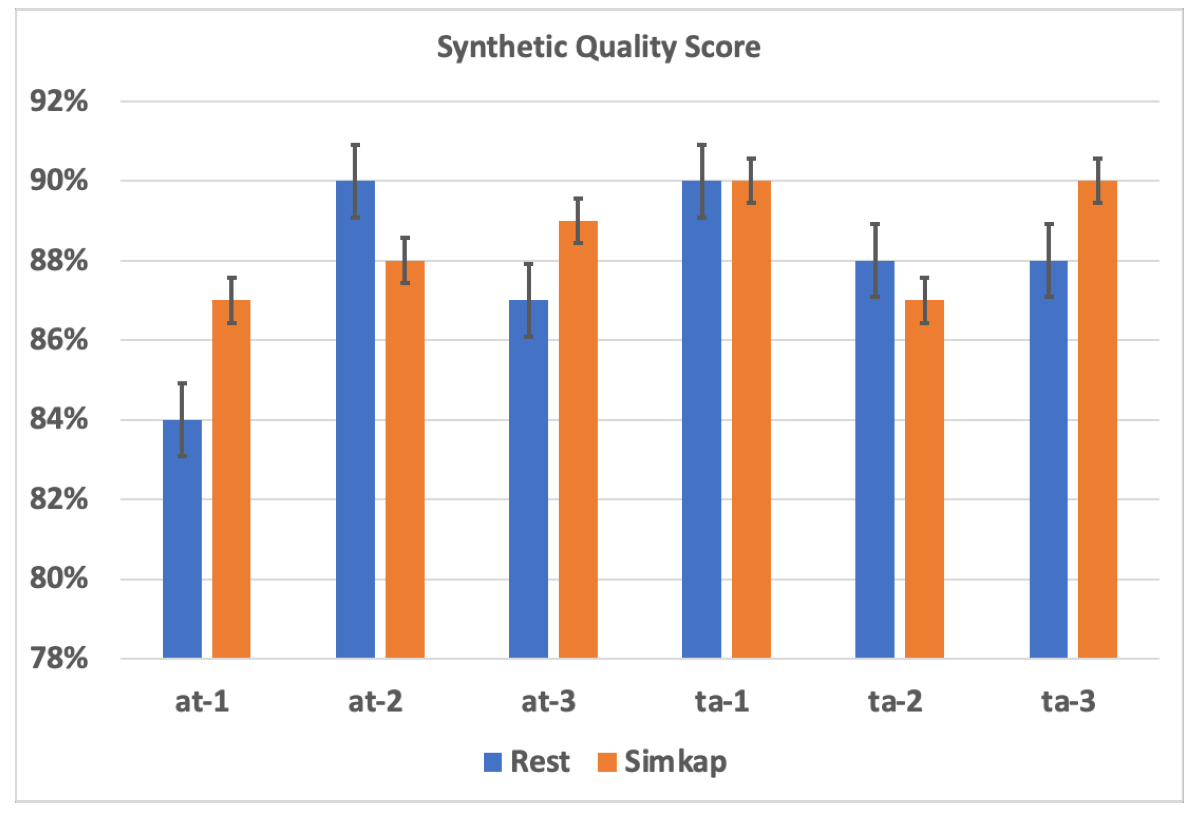
4.3. Training Set Evaluation across Indexes

The “curse of dimensionality” issue arose due to the low number of training instances compared to the independent features. During the initial model evaluation with test data, the average accuracy was only 60%. The classifiers’ learning curves indicated that the model was underfitting and could not generalize from test data. To overcome the bias caused by the small variance in data, synthetic data generation was used to train more accurate models. The study utilized the initial dataset of 48 subjects, with 150 data points (2.5 min of EEG activity divided into 150 segments of 1 s) for each of the indexes designed in Equation (2). Two synthetic datasets were generated, one for the “Rest” and “Simkap” task load conditions, respectively, to preserve the original dataset’s characteristics. The findings indicated a synthetic quality score of more than 87% for all the chosen objectives and continuous mental workload indexes, demonstrating excellent quality and similarity to other research studies [61]. As a result, data were synthesized for an additional 180 subjects, generating 150 data points each for every mental workload index. Therefore, the final dataset includes both original and synthesized data, with 228 subjects and 150 data points for each mental workload index as defined in Equation (2). Figure 4 displays the quality scores for synthetic data for “Rest” and “Simkap” conditions, respectively.

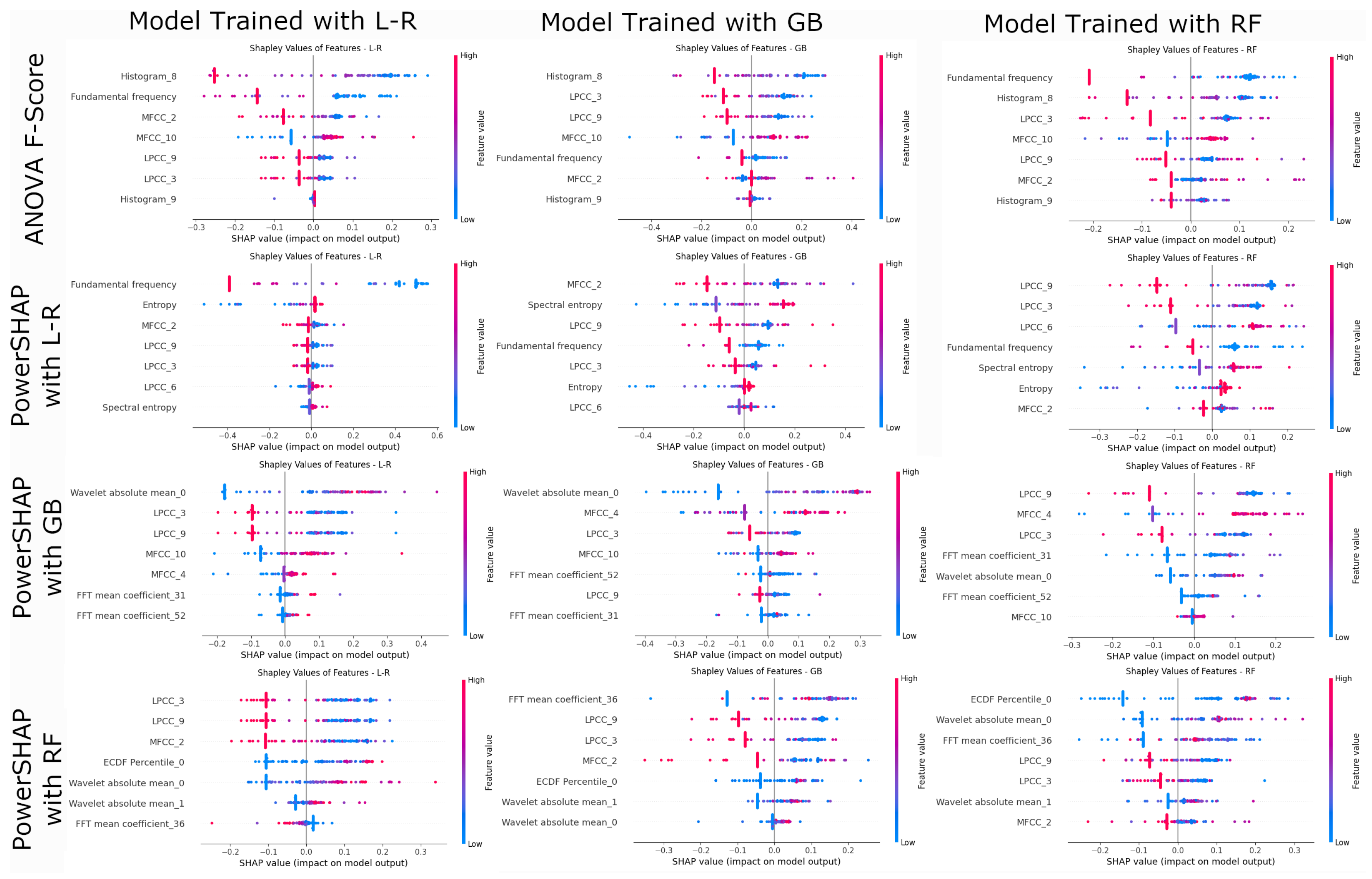
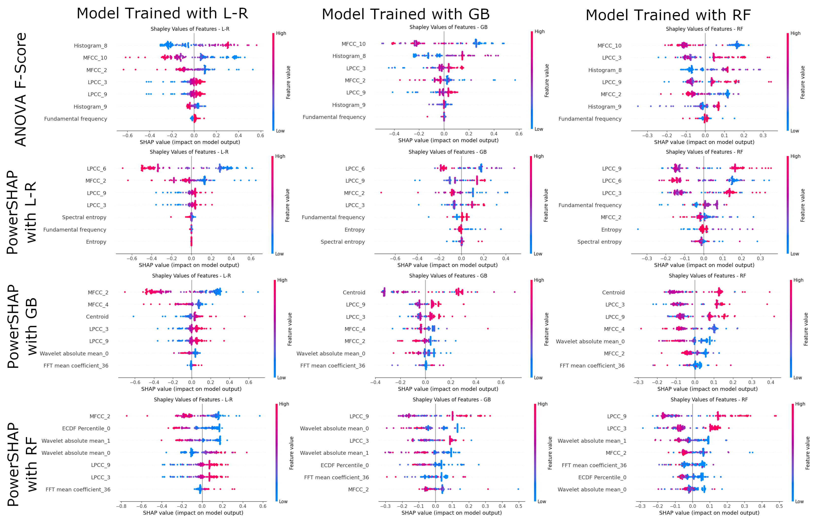
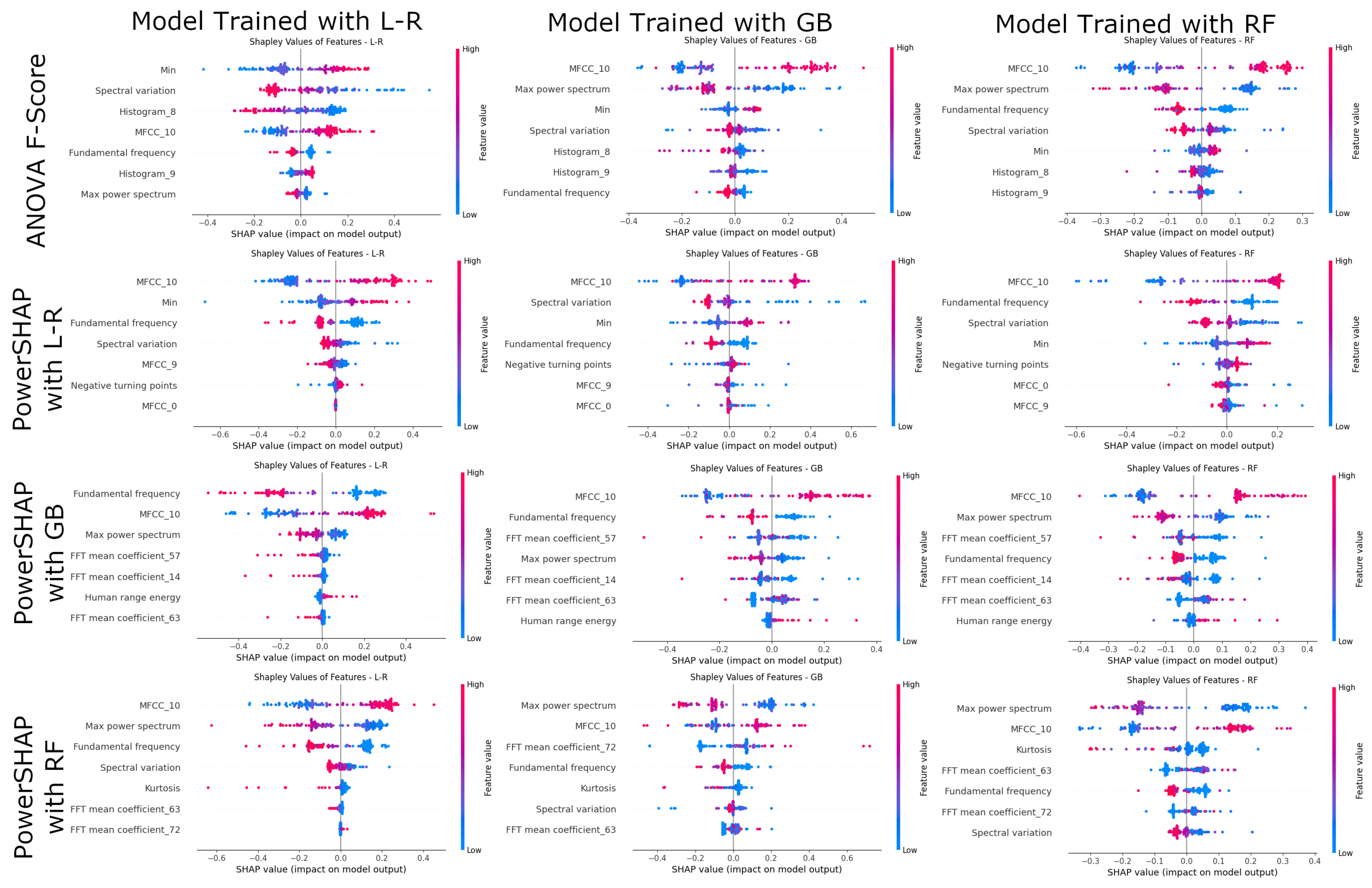
4.4. Model Explainability and Validation

Figure 5 showcases the classifiers’ performance and the evaluation metrics for all mental workload objective indexes. The dashed red line depicts the threshold for below and above-average model performance, set at 90%.
Based on the figure data analysis, it is evident that the Shapley-based feature selection methods utilizing PowerSHAP with Logistic Regression (L-R) and Gradient Boosting (GB) demonstrated an exceptional performance for the mental workload index at-3. Furthermore, the PowerSHAP feature selection techniques utilized for theta-to-alpha ratio indexes ta-2 and ta-3 have shown an above-average performance of 90% when trained with Linear Regression and Gradient Boosting. However, the PowerSHAP features trained with Random Forest performance seems below the average threshold. On the other hand, the statistical feature selection method has shown a below-average performance of 90% across all mental workload objective indexes. To better analyze the results and see the model performance of the aforementioned ratios for both feature selection methods, Figure 6 outlines the density plots of the model training with Monte Carlo sampling provided in Section 3.5.
Figure 6 shows a better performance of the PowerSHAP feature selection methods for the mental workload indexes at-3, ta-2, and ta-3. Furthermore, the mental workload index at-1 very clearly shows the best performance of the powerSHAP feature selection method compared to ANOVA F-score, even though the model’s overall performance is below the mean threshold of 90%, as given in Figure 5. Table 3 showcases the two-tailed t-test results for model performance accuracy between ANOVA F-score and Shapley-based Powershap feature selection methods across all workload objective indexes.
We analyzed the effect size of the density plots using Cohen’s d to determine the significance levels presented in Table 3. Cohen’s d is a standardized measurement used to determine the difference between the means of two groups. It is utilized to compare a sample from PowerSHAP feature selection methods with the ANOVA feature selection method to validate the significance levels in Table 3. Cohen’s d is an appropriate effect size alongside t-tests and ANOVA analyses. Table 3 shows medium and large effect sizes for the at-2, ta-2, and ta-3 mental workload indexes. Furthermore, very strong effect sizes are seen in at-1, even though the model performance for that index is under the threshold of 90%. To comprehensively analyze the models, we will thoroughly examine the significant feature selection methods outlined in Table 3. Furthermore, we will examine the top-performing indexes as per Figure 5, particularly at-3, ta-2, and ta-3. To better understand the crucial features and their characteristics, Table 4 provides a detailed overview of these features and their descriptions as they apply to our analysis.
Figure 7 in the at-3 workload index clearly illustrates the importance of features as determined by feature selection methods. In addition, Figure 8 confidently presents the model explainability of feature importance through Shapley values in the form of beeswarm plots generated from the test set.
Figure 7 and Figure 8 revealed an interesting observation. During the feature selection process using ANOVA f-score, “Histogram_9” and “Histogram_8” had the highest f-score value, suggesting they were the most important features. However, upon examining the model’s feature contributions using Shapley values, “Histogram_8”, “Fundamental_frequency” and “LPCC_3” were the top four critical features. It is quite observable that “Histogram_9”, which was the top ranking feature with ANOVA f-score selection method, when explained by SHAP, rank as the least contributing feature across all training methods (L-R, GB, and RF). When using PowerSHAP with L-R for feature selection, “spectral entropy” and “Entropy” features appear as the most important ones when selected using PowerSHAP with L-R. However, Shapley values retired with Shapley additive explanations showed “LPCC_9”, “LPCC_3”, “MFCC_9”, and “Fundamental_frequency” that contributed the most to the model’s output. When features are analyzed for the cases of feature selection methods using PowerSHAP with both Gradient Boosting (GB) and Random Forest (RF), we observe “FFT Mean Coefficient_52”, “MFCC_10”, “EDCF Percentile_0”, and “Vawelet absolute mean_1” as the most important features. However, the model explainability provided with SHAP, brings the least important features from the feature selection method as the highest contributing ones. Features like “MFCC_4”, “Wavelet absolute mean_0”, and “LPCC_9” are the least ranked ones from the feature selection method; however, they appear as the most contributing ones appearing in the top two of most contributing features. Figure 9 shows the feature importance for the ta-2 workload index, and Figure 10 illustrates the model’s explainability in terms of feature importance through the Shapley values generated from the test set in beeswarm plots.
When analyzing the ta-2 mental workload index, we found that “Histogram_9” and “Histogram_8” were the most important features during ANOVA F-score feature selection. However, when explaining the contribution of features to the model output, “MFCC_10” and “LPCC_3” (Linear Prediction Cepstral Coefficients 3) also have the greatest impact along “Histogram_8”. In the case of features selected with PowerSHAP+L-R and trained with L-R, GB, and RF, “MFCC_2”, “LPCC_6”, and “LPCC_9” (MEL Cepstral Coefficients 2 and Linear Prediction Cepstral Coefficients 6 and 9) are the most important features, despite being ranked relatively low in importance during feature selection. Another crucial observation is that highly ranked features during feature selection, like “Spectral Entropy” and “Entropy”, are at the bottom of features that contribute to model output when explained with Shapley values. For features selected with PowerSHAP + GB and PowerSHAP + RF and trained with L-R, GB, and RF, the “LPCC_9” and “MFCC_2” features were found to be the most important for model explainability with test data. Even though “LPCC_3” and “LPCC_9” were ranked at the bottom in both cases, they were among the top three features contributing to the model output during model training and explainability with Shapley values. In reference to the ta-3 workload index, Figure 11 shows the feature importance as determined by feature selection methods.
The Shapley values generated from the test set are presented as beeswarm plots in Figure 12, depicting the model explainability of feature importance.
For the theta-to-alpha (ta-3) workload index, the feature MFCC_10 (MEL cepstral coefficients 10) is ranked at the bottom during feature selection using all statistical and Shapley-based feature selection methods. However, upon analyzing the Shapley value for their impact on the model output, it was found that this feature had the highest contribution across the board in all models explained with Shapley Additive Explanations.

5. Discussion

The findings presented in this paper suggest that using Shapley-value-based methods for model training leads to better performance than using statistical methods with an ANOVA F-score. This is particularly evident in the mental workload indexes at-3, ta-2, and ta-3. Additionally, the results from Table 3 demonstrate a statistically significant difference between ANOVA F-score and PowerSHAP methods, confirming the hypothesis outlined in Section 3 that high-level EEG features selected using the Shapley-based method have a greater impact on model performance for discriminating the self-reported perception of mental workload than statistical methods. When we analyze model explainability using SHAP, we notice an intriguing observation by comparing the features selected through both methods. When presented with testing data, the less important features tend to impact the model output significantly. Features such as “Wavelet absolute mean_0”, “Wavelet absolute mean_1”, and “Fundamental frequency”, statistical histogram features like “Histogram_8” and “Linear" and MEL cepstral coefficients (“LPCC_3”, “LPCC_6”, “LPCC_9”, and “MFCC_10”) contribute the most to the model output in all trained and evaluated models. In Figure 13, we can compare the ranked features from feature selection methods (ANOVA F-score and PowerSHAP) and their respective contribution to the model output. The feature importance is normalized between the [ 0 1 ] range, where zero indicates a low impact of the feature on training, and one indicates a high impact.
Looking at Figure 13, we can observe a discrepancy between the features selected through the ANOVA F-score, namely “Histogram_8” and “MFCC_10”, and those that contribute the most to the model output. Interestingly, the high-ranked features from ANOVA F-score appear to be the least important in model explainability and vice versa. This trend is also visible in the “linear and MEL cepstral coefficients” (“LPCC_3”, “LPCC_9”, and “MFCC_10”) for both feature selection methods and their respective feature importance for model explainability.
The importance of Shapley values in model explainability is highlighted in the research. It is observed that people tend to trust the model explainability provided by Shapley values. This claim is based on the following points:
  • Methods based on Shapley values are not tied to any specific machine learning model and can be used with linear and nonlinear models, decision trees, and neural networks. These methods are effective, as they avoid common mistakes such as using a “one-size-fits-all” approach to interpretability, poor model generalization, over-reliance on complex models for explainability, and neglecting feature dependence [62]. On the other hand, statistical feature selection methods often require a particular model or make assumptions about data distribution.
  • When working with complex datasets, Shapley-based methods are crucial as they consider the interaction between features. On the other hand, statistical feature selection techniques like correlation-based feature selection only consider pairwise correlations between features and may overlook significant interactions.
  • Regarding ranking features, Shapley-based methods are more reliable because small changes do not easily influence them in the data or model. On the other hand, statistical feature selection methods may yield different results depending on the particular data sample or model being utilized.
  • Methods based on Shapley values are useful in clearly understanding each feature’s importance. This is because it highlights the contribution of a feature to the prediction, making it easy to explain to domain experts. On the other hand, statistical feature selection methods may require an easily interpretable feature importance measure.
Even though Shapley-based feature selection methods are more effective than statistical methods, there are still some open research questions and inconclusive explanations regarding contradictory results. This is because the feature importance in the selection method may differ from the feature importance of the model output provided by SHAP. Some researchers argue that using Shapley values for feature importance in machine learning models can lead to mathematical problems which may increase complexity and the need for causal reasoning. Moreover, Shapley values should be able to explain their results in a way that aligns with human-centric goals of explainability [63]. One particular study suggests that using model averaging directly for feature selection requires caution, as the average performance of a feature across all submodels may not reflect its specific performance in the optimal submodels. To ensure the selection of all features based on their optimal submodel contributions, it is best to select all features explicitly [44]. Furthermore, the authors demonstrate this claim with examples outlined through sets of axioms like efficiency, additivity, and balanced contributions. It is possible that the contradictions between feature selection methods and feature contributions, as seen in Figure 13, could be attributed to the direct averaging of features during Shapley Additive Explanations (SHAP) and the Monte Carlo simulation used during training. However, further research is necessary to confirm this hypothesis.

6. Conclusions

The paper outlined the need for a more comprehensive understanding of the performance and interpretability of different feature selection methods in machine learning models that discriminate self-reported perceptions of mental workload using EEG band ratios. This research issue is tackled through a comparative empirical study using a six-step process pipeline as outlined in Section 3. Logistic Regression (L-R), Gradient Boosting (GB), and Random Forest (RF) learning techniques were employed to train the models, with a focus on utilizing Shapley-based and ANOVA F-score feature selection methods. To ensure model explainability, we utilized Shapley Additive Explanations.
According to the analysis, it was discovered that feature selection methods that utilize Shapley values can improve model performance and partially explain how the model can distinguish between different mental workload perceptions using EEG data. These methods can identify the most crucial features and their corresponding impact on the model’s predictions, thereby providing valuable insights into the factors contributing to successfully identifying mental workload perceptions through machine learning. In identifying the most impactful features contributing to model output, the study uncovered unexpected contradictions between the Shapley-based feature selection methods (PowerSHAP and ANOVA F-score) and the Shapley Additive Explanation (SHAP) method. It is important to note that possible explanations for these contradictions are hypothesized in Section 5, and further research will be necessary to validate these claims. Although the paper demonstrated that Shapley-based methods outperform traditional statistical approaches, it should be noted that Shapley-based feature selection methods can often lead to complex and inconclusive interpretations. This is due to the complex interplay between the perceived importance of features during the selection process and their actual significance in shaping the final output of the model. However, these conflicting outcomes provide valuable insights into the intricate dynamics of feature importance and model behavior. Therefore, it is essential to acknowledge these potential disparities when working with feature selection, as it can lead to a more comprehensive understanding of the model’s inner workings and pave the way for refined methodologies that harness the true power of Shapley-based techniques.
It is important to note that this research has limitations in terms of the feature selection methods used to explain the models. This study focuses on statistical (ANOVA-F-score) and game theoretic (PowerSHAP) approaches. However, there are other selection methods based on explainable AI, such as wrapper-based selectors like Boruta, selection methods based on regression models or random forest, iterative dataset weighting, and targeted replacement values. The rationale behind using statistical and Shapley-based methods is that they have been proven to effectively select essential features and discard non-contributing ones, which not only maintains or improves classification accuracy, but also reduces the execution time in machine learning models, making the Shapley-based feature selection effective and efficient [64]. Additionally, Shapley values are relatively consistent across selected machine learning models, making the analysis of model explainability more straightforward. It is also essential to acknowledge that the explanations may vary depending on the model’s outcome and application, as outlined in this study.
In future investigations, researchers can thoroughly examine the properties of these features to construct models that can precisely evaluate the model’s accuracy. More research will elaborate on how the alpha-to-theta and theta-to-alpha ratio indexes can be employed to explain the model’s efficiency regarding the following concerns. The first is a further confirmation of the findings of this study, aiming at replicating the experiment using additional publicly available datasets. The second is to enhance the explainability of models utilizing additional additive methods, such as LIME, DeepLIFT, and Layer-wise relevance estimation, in addition to the traditional Shapley value estimation.

Author Contributions

Conceptualization, B.R. and L.L.; methodology, B.R. and L.L.; software, B.R.; validation, B.R.; formal analysis, B.R. and L.L.; investigation, B.R.; resources, B.R.; data curation, B.R.; writing—original draft preparation, B.R.; writing—review and editing, B.R. and L.L.; visualization, B.R.; supervision, L.L.; project administration, B.R.; funding acquisition, L.L. All authors have read and agreed to the published version of the manuscript.

Funding

Supported by MCSA Post-doc CareerFIT fellowship, funded by Enterprise Ireland, TU Dublin School of Computer Science and the European Commission. Fellowship ref. number: MF2020 0144.

Institutional Review Board Statement

Not applicable.

Informed Consent Statement

Not applicable.

Data Availability Statement

Publicly available datasets were analyzed in this study. These data can be found here: [https://github.com/braufi/xai-2023-supplemental/tree/f6b3a9272a8dd63303634d858564ecb8ac2cf7f8 (accessed on 15 December 2023)].

Conflicts of Interest

The authors declare no conflicts of interest with this manuscript. The funders had no role in the study’s design; in the collection, analyses, or interpretation of data; in the writing of the manuscript; or in the decision to publish the results.

References

  1. Lundberg, S.M.; Lee, S.-I. A unified approach to interpreting model predictions. Adv. Neural Inf. Process. Syst. 2017, 30, 4765–4774. [Google Scholar]
  2. Wang, J.; Jenna, W.; Scott, L. Shapley flow: A graph-based approach to interpreting model predictions. In Proceedings of the International Conference on Artificial Intelligence and Statistics, Virtual, 13–15 April 2021. [Google Scholar]
  3. Sim, R.H.L.; Xu, X.; Low, B.K.H. Data valuation in machine learning: “ingredients”, strategies, and open challenges. In Proceedings of the IJCAI, Vienna, Austria, 23–29 July 2022. [Google Scholar]
  4. Zacharias, J.; von Zahn, M.; Chen, J.; Hinz, O. Designing a feature selection method based on explainable artificial intelligence. Electron. Mark. 2022, 32, 2159–2184. [Google Scholar] [CrossRef]
  5. Cohen, S.; Dror, G.; Ruppin, E. Feature selection via coalitional game theory. Neural Comput. 2007, 19, 1939–1961. [Google Scholar] [CrossRef] [PubMed]
  6. Rozemberczki, B.; Watson, L.; Bayer, P.; Yang, H.T.; Kiss, O.; Nilsson, S.; Sarkar, R. The shapley value in machine learning. arXiv 2022, arXiv:2202.05594. [Google Scholar]
  7. Wang, J.; Wiens, J.; Flow, S.L.S. A Graph-based Approach to Interpreting Model Predictions. arXiv 2020, arXiv:2010.14592. [Google Scholar]
  8. Sundararajan, M.; Najmi, A. The many Shapley values for model explanation. In Proceedings of the International Conference on Machine Learning, Virtual, 13–18 July 2020; pp. 9269–9278. [Google Scholar]
  9. Covert, I.; Lee, S.I. Improving KernelSHAP: Practical Shapley value estimation using linear regression. In Proceedings of the International Conference on Artificial Intelligence and Statistics, Virtual, 13–15 April 2021. [Google Scholar]
  10. Shapley, L.S. A Value for n-Person Games. In Contributions to the Theory of Games (AM-28); Kuhn, H., Tucker, A., Eds.; Princeton University Press: Princeton, NJ, USA, 1953; Volume II, pp. 307–318. [Google Scholar] [CrossRef]
  11. Chalkiadakis, G.; Elkind, E.; Wooldridge, M. Computational Aspects of Cooperative Game Theory. Synth. Lect. Artif. Intell. Mach. Learn. 2011, 5, 1–168. [Google Scholar]
  12. Dondio, P.; Longo, L. Trust-based techniques for collective intelligence in social search systems. In Next Generation Data Technologies for Collective Computational Intelligence; Springer: Berlin/Heidelberg, Germany, 2011; pp. 113–135. [Google Scholar]
  13. Shrikumar, A.; Greenside, P.; Kundaje, A. Learning important features through propagating activation differences. In Proceedings of the International conference on Machine Learning, Sydney, NSW, Australia, 6–11 August 2017; pp. 3145–3153. [Google Scholar]
  14. Merrick, L.; Taly, A. The explanation game: Explaining machine learning models using shapley values. In Proceedings of the Machine Learning and Knowledge Extraction: 4th IFIP TC 5, TC 12, WG 8.4, WG 8.9, WG 12.9 International Cross-Domain Conference, CD-MAKE 2020, Dublin, Ireland, 25–28 August 2020; Proceedings 4. Springer International Publishing: Berlin/Heidelberg, Germany, 2020; pp. 17–38. [Google Scholar]
  15. Louhichi, M.; Nesmaoui, R.; Mbarek, M.; Lazaar, M. Shapley Values for Explaining the Black Box Nature of Machine Learning Model Clustering. Procedia Comput. Sci. 2023, 220, 806–811. [Google Scholar] [CrossRef]
  16. Tripathi, S.; Hemachandra, N.; Trivedi, P. Interpretable feature subset selection: A Shapley value based approach. In Proceedings of the 2020 IEEE International Conference on Big Data (Big Data), Atlanta, GA, USA, 10–13 December 2020; pp. 5463–5472. [Google Scholar]
  17. Främling, K.; Westberg, M.; Jullum, M.; Madhikermi, M.; Malhi, A. Comparison of contextual importance and utility with lime and Shapley values. In Proceedings of the Explainable and Transparent AI and Multi-Agent Systems: Third International Workshop, EXTRAAMAS 2021, Virtual Event, 3–7 May 2021; pp. 39–54. [Google Scholar]
  18. Longo, L.; Brcic, M.; Federico, C.; Jaesik, C.; Confalonieri, R.; Del Ser, J.; Guidotti, R.; Hayashi, Y.; Herrera, F.; Holzinger, A.; et al. Explainable Artificial Intelligence (XAI) 2.0: A manifesto of open challenges and interdisciplinary research directions. Inf. Fusion 2024, 106, 102301. [Google Scholar] [CrossRef]
  19. Zhang, J.; Xia, H.; Sun, Q.; Liu, J.; Xiong, L.; Pei, J.; Ren, K. Dynamic Shapley Value Computation. In Proceedings of the 2023 IEEE 39th International Conference on Data Engineering (ICDE), Anaheim, CA, USA, 3–7 April 2023; pp. 639–652. [Google Scholar]
  20. Jia, R.; Dao, D.; Wang, B.; Hubis, F.A.; Hynes, N.; Gürel, N.M.; Spanos, C.J. Towards efficient data valuation based on the shapley value. In Proceedings of the The 22nd International Conference on Artificial Intelligence and Statistics, Naha, Japan, 16–18 April 2019; pp. 1167–1176. [Google Scholar]
  21. Ancona, M.; Ceolini, E.; Öztireli, C.; Gross, M. Towards better understanding of gradient-based attribution methods for deep neural networks. arXiv 2017, arXiv:1711.06104. [Google Scholar]
  22. Gevins, A.; Smith, M.E. Neurophysiological measures of cognitive workload during human–computer interaction. Theor. Issues Ergon. Sci. 2003, 4, 113–131. [Google Scholar] [CrossRef]
  23. Borghini, G.; Astolfi, L.; Vecchiato, G.; Mattia, D.; Babiloni, F. Measuring neurophysiological signals in aircraft pilots and car drivers for the assessment of mental workload, fatigue and drowsiness. Neurosci. Biobehav. Rev. 2014, 44, 58–75. [Google Scholar] [CrossRef]
  24. Fernandez Rojas, R.; Debie, E.; Fidock, J.; Barlow, M.; Kasmarik, K.; Anavatti, S.; Abbass, H. Electroencephalographic workload indicators during teleoperation of an unmanned aerial vehicle shepherding a swarm of unmanned ground vehicles in contested environments. Front. Neurosci. 2020, 14, 40. [Google Scholar] [CrossRef]
  25. Raufi, B.; Longo, L. An Evaluation of the EEG alpha-to-theta and theta-to-alpha band Ratios as Indexes of Mental Workload. Front. Neuroinform. 2022, 16, 44. [Google Scholar] [CrossRef] [PubMed]
  26. Raufi, B. Hybrid models of performance using mental workload and usability features via supervised machine learning. In Proceedings of the Human Mental Workload: Models and Applications: Third International Symposium, H-WORKLOAD 2019, Rome, Italy, 14–15 November 2019; Springer International Publishing: Berlin/Heidelberg, Germany, 2019; pp. 136–155. [Google Scholar]
  27. Mohanavelu, K.; Poonguzhali, S.; Janani, A.; Vinutha, S. Machine learning-based approach for identifying mental workload of pilots. Biomed. Signal Process. Control 2022, 75, 103623. [Google Scholar] [CrossRef]
  28. Kakkos, I.; Dimitrakopoulos, G.N.; Sun, Y.; Yuan, J.; Matsopoulos, G.K.; Bezerianos, A.; Sun, Y. EEG fingerprints of task-independent mental workload discrimination. IEEE J. Biomed. Health Inform. 2021, 25, 3824–3833. [Google Scholar] [CrossRef]
  29. Longo, L. Designing medical interactive systems via assessment of human mental workload. In Proceedings of the 2015 IEEE 28th International Symposium on Computer-Based Medical Systems, Sao Carlos, Brazil, 22–25 June 2015; pp. 364–365. [Google Scholar]
  30. Longo, L.; Rajendran, M. A novel parabolic model of instructional efficiency grounded on ideal mental workload and performance. In Proceedings of the 5th International Symposium, H-WORKLOAD 2021, Virtual Event, 24–26 November 2021; pp. 11–36. [Google Scholar]
  31. Longo, L. Formalising human mental workload as non-monotonic concept for adaptive and personalised web-design. In Proceedings of the International Conference on User Modeling, Adaptation, and Personalization, Montreal, QC, Canada, 16–20 July 2012. [Google Scholar]
  32. Jafari, M.J.; Zaeri, F.; Jafari, A.H.; Payandeh Najafabadi, A.T.; Al-Qaisi, S.; Hassanzadeh-Rangi, N. Assessment and monitoring of mental workload in subway train operations using physiological, subjective, and performance measures. Hum. Factors Ergon. Manuf. Serv. Ind. 2020, 30, 165–175. [Google Scholar] [CrossRef]
  33. Longo, L.; Barrett, S. A computational analysis of cognitive effort. In Proceedings of the Asian Conference on Intelligent Information and Database Systems, Hue City, Vietnam, 24–26 March 2010. [Google Scholar]
  34. Hancock, G.M.; Longo, L.; Young, M.S.; Hancock, P.A. Mental Workload. Handbook of Human Factors and Ergonomics; Wiley Online Library: Hoboken, NJ, USA, 2021. [Google Scholar]
  35. Longo, L.; Wickens, C.D.; Hancock, G.; Hancock, P.A. Human Mental Workload: A Survey and a Novel Inclusive Definition. Front. Psychol. 2022, 13, 883321. [Google Scholar] [CrossRef]
  36. Käthner, I.; Wriessnegger, S.C.; Müller-Putz, G.R.; Kübler, A.; Halder, S. Effects of mental workload and fatigue on the P300, alpha and theta band power during operation of an ERP (P300) brain–computer interface. J. Biol. Psychiatry 2014, 102, 118–129. [Google Scholar] [CrossRef] [PubMed]
  37. Muñoz-de-Escalona, E.; Cañas, J.J.; Leva, C.; Longo, L. Task demand transition peak point effects on mental workload measures divergence. In Proceedings of the Human Mental Workload: Models and Applications: 4th International Symposium, H-WORKLOAD 2020, Granada, Spain, 3–5 December 2020; Springer International Publishing: Berlin/Heidelberg, Germany, 2020; pp. 207–226. [Google Scholar]
  38. Longo, L. Modeling Cognitive Load as a Self-Supervised Brain Rate with Electroencephalography and Deep Learning. Brain Sci. 2022, 12, 1416. [Google Scholar] [CrossRef]
  39. Rizzo, L. Middeldorf and Longo, Luca, Representing and inferring mental workload via defeasible reasoning: A comparison with the NASA Task Load Index and the Workload Profile. In Proceedings of the 1st Workshop on Advances in Argumentation in Artificial Intelligence AI3@AI*IA, Bari, Italy, 14–17 November 2017. [Google Scholar]
  40. Rizzo, L.; Luca, L. Inferential Models of Mental Workload with Defeasible Argumentation and Non-monotonic Fuzzy Reasoning: A Comparative Study. In Proceedings of the 2nd Workshop on Advances in Argumentation in Artificial Intelligence, Co-Located with XVII International Conference of the Italian Association for Artificial Intelligence, AI3@AI*IA 2018, Trento, Italy, 20–23 November 2018; pp. 11–26. [Google Scholar]
  41. Hoque, N.; Bhattacharyya, D.K.; Kalita, J.K. MIFS-ND: A mutual information-based feature selection method. Expert Syst. Appl. 2014, 41, 6371–6385. [Google Scholar] [CrossRef]
  42. Zhai, Y.; Song, W.; Liu, X.; Liu, L.; Zhao, X. A chi-square statistics based feature selection method in text classification. In Proceedings of the 2018 IEEE 9th International Conference on Software Engineering and Service Science (ICSESS), Beijing, China, 23–25 November 2018; pp. 160–163. [Google Scholar]
  43. Perangin-Angin, D.J.; Bachtiar, F.A. Classification of Stress in Office Work Activities Using Extreme Learning Machine Algorithm and One-Way ANOVA F-Test Feature Selection. In Proceedings of the 2021 4th International Seminar on Research of Information Technology and Intelligent Systems (ISRITI), Yogyakarta, Indonesia, 16–17 December 2021; pp. 503–508. [Google Scholar]
  44. Fryer, D.; Strümke, I.; Nguyen, H. Shapley Values for Feature Selection The Good, the Bad, and the Axioms. arXiv 2021, arXiv:2102.10936. [Google Scholar] [CrossRef]
  45. Williamson, B.; Feng, J. Efficient nonparametric statistical inference on population feature importance using Shapley values. In Proceedings of the International Conference on Machine Learning, Virtual, 13–18 July 2020; pp. 10282–10291. [Google Scholar]
  46. Junaid, M.; Ali, S.; Eid, F.; El-Sappagh, S.; Abuhmed, T. Explainable machine learning models based on multimodal time-series data for the early detection of Parkinson’s disease. Comput. Methods Programs Biomed. 2023, 234, 107495. [Google Scholar] [CrossRef]
  47. Msonda, J.R.; He, Z.; Lu, C. Feature Reconstruction Based Channel Selection for Emotion Recognition Using EEG. In Proceedings of the 2021 IEEE Signal Processing in Medicine and Biology Symposium, 2021 (SPMB), Philadelphia, PA, USA, 4 December 2021; pp. 1–7. [Google Scholar]
  48. Moussa, M.M.; Alzaabi, Y.; Khandoker, A.H. Explainable computer-aided detection of obstructive sleep apnea and depression. IEEE Access 2022, 10, 110916–110933. [Google Scholar] [CrossRef]
  49. Khosla, A.; Khandnor, P.; Chand, T. Automated diagnosis of depression from EEG signals using traditional and deep learning approaches: A comparative analysis. Biocybern. Biomed. Eng. 2022, 42, 108–142. [Google Scholar] [CrossRef]
  50. Shanarova, N.; Pronina, M.; Lipkovich, M.; Ponomarev, V.; Müller, A.; Kropotov, J. Application of Machine Learning to Diagnostics of Schizophrenia Patients Based on Event-Related Potentials. Diagnostics 2023, 13, 509. [Google Scholar] [CrossRef] [PubMed]
  51. Islam, R.; Andreev, A.V.; Shusharina, N.N.; Hramov, A.E. Explainable machine learning methods for classification of brain states during visual perception. Mathematics 2022, 10, 2819. [Google Scholar] [CrossRef]
  52. Kaczorowska, M.; Plechawska-Wójcik, M.; Tokovarov, M. Interpretable machine learning models for three-way classification of cognitive workload levels for eye-tracking features. Brain Sci. 2021, 11, 210. [Google Scholar] [CrossRef]
  53. Lim, W.L.; Sourina, O.; Wang, L.P. STEW: Simultaneous task EEG workload data set. IEEE Trans. Neural Syst. Rehabil. Eng. 2018, 26, 2106–2114. [Google Scholar] [CrossRef]
  54. Mikayoshi, M. Makoto’s Preprocessing Pipeline. 2018. Available online: https://sccn.ucsd.edu/wiki/Makotoś_preprocessing_pipeline (accessed on 4 April 2023).
  55. Nolan, H.; Whelan, R.; Reilly, R.B. FASTER: Fully automated statistical thresholding for EEG artifact rejection. J. Neurosci. Methods 2010, 192, 152–162. [Google Scholar] [CrossRef]
  56. Verhaeghe, J.; Van Der Donckt, J.; Ongenae, F.; Van Hoecke, S. Powershap: A power-full shapley feature selection method. In Proceedings of the Machine Learning and Knowledge Discovery in Databases: European Conference, ECML PKDD 2022, Grenoble, France, 19–23 September 2022; Springer International Publishing: Cham, Switzerland, 2022; pp. 71–87. [Google Scholar]
  57. Lieberman, M.G.; Morris, J.D. The precise effect of multicollinearity on classification prediction. Mult. Linear Regres. Viewpoints 2014, 40, 5–10. [Google Scholar]
  58. Mridha, K.; Kumar, D.; Shukla, M.; Jani, M. Temporal features and machine learning approaches to study brain activity with EEG and ECG. In Proceedings of the 2021 International Conference on Advance Computing and Innovative Technologies in Engineering (ICACITE), Greater Noida, India, 4–5 March 2021; pp. 409–414. [Google Scholar]
  59. Goodfellow, I.; Pouget-Abadie, J.; Mirza, M.; Xu, B.; Warde-Farley, D.; Ozair, S.; Bengio, Y. Generative adversarial networks. Commun. ACM 2020, 63, 139–144. [Google Scholar] [CrossRef]
  60. Frølich, L.; Dowding, I. Removal of muscular artifacts in EEG signals: A comparison of linear decomposition methods. Brain Inform. 2018, 5, 13–22. [Google Scholar] [CrossRef] [PubMed]
  61. Hernandez-Matamoros, A.; Fujita, H.; Perez-Meana, H. A novel approach to create synthetic biomedical signals using BiRNN. Inf. Sci. 2020, 541, 218–241. [Google Scholar] [CrossRef]
  62. Molnar, C.; König, G.; Herbinger, J.; Freiesleben, T.; Dandl, S.; Scholbeck, C.A.; Bischl, B. General pitfalls of model-agnostic interpretation methods for machine learning models. In Proceedings of the xxAI-Beyond Explainable AI: International Workshop, Held in Conjunction with ICML 2020, Vienna, Austria, 18 July 2020; Revised and Extended Papers. Springer International Publishing: Cham, Switzerland, 2022; pp. 39–68. [Google Scholar]
  63. Kumar, I.E.; Venkatasubramanian, S.; Scheidegger, C.; Friedler, S. Problems with Shapley-value-based explanations as feature importance measures. In Proceedings of the International Conference on Machine Learning, Virtual, 21 November 2020; pp. 5491–5500. [Google Scholar]
  64. Bolón-Canedo, V.; Sánchez-Maroño, N.; Alonso-Betanzos, A. Distributed feature selection: An application to microarray data classification. Appl. Soft Comput. 2015, 30, 136–150. [Google Scholar] [CrossRef]
Figure 1. A step–by–step illustration for classifying self-reported mental workload perception using mental workload indexes created through the EEG analysis of the alpha and theta bands. (A) Signal denoising process. (B) Select electrodes from the frontal cortical areas for the theta band and the parietal cortical areas for the alpha band and group them to create electrode clusters. (C) Calculate the mental workload indexes using the alpha-to-theta and theta-to-alpha band ratios. (D) Extract high-level features from the mental workload indexes. (E) Use ANOVA F-Score and PowerSHAP to select the best features. (F) Train a machine learning model for classifying self-reported mental workload perception. (G) Evaluate the model. (H) Explain the model for hypothesis testing.
Biomedinformatics 04 00048 g001
Figure 2. A step–by–step illustration of the model training procedure, evaluation and explanation for each feature selection method.
Biomedinformatics 04 00048 g002
Figure 3. Pearson correlation of features selected with SelectKBest and PowerSHAP for the case of at-2 mental workload index.
Biomedinformatics 04 00048 g003
Figure 4. Quality scores of synthetic data for “rest” and “Simkap” task load conditions.
Biomedinformatics 04 00048 g004
Figure 5. Model performance for features selected with ANOVA F-score and PowerSHAP methods.
Biomedinformatics 04 00048 g005
Figure 6. Density plots of model performance for features selected with ANOVA F-score and PowerSHAP methods. The comparison is made between ANOVA F-Score against PowerSHAP with L-R, GB, and RF, respectively.
Biomedinformatics 04 00048 g006
Figure 7. Feature importances selected from ANOVA F-score and PowerSHAP for the case of at-3.
Biomedinformatics 04 00048 g007
Figure 8. Shapley values on feature impact on model output selected with ANOVA F-score and PowerSHAP and trained with L-R, GB, and RF for the case of at-3.
Biomedinformatics 04 00048 g008
Figure 9. Feature importances selected from ANOVA F-score and PowerSHAP for the case of ta-2.
Biomedinformatics 04 00048 g009
Figure 10. Shapley values on feature impact on model output selected with ANOVA F-score and PowerSHAP and trained with L-R, GB, and RF for the case of ta-2.
Biomedinformatics 04 00048 g010
Figure 11. Feature importances selected from ANOVA F-score and PowerSHAP for the case of ta-3.
Biomedinformatics 04 00048 g011
Figure 12. Shapley values on feature impact on model output selected with ANOVA F-score and PowerSHAP and trained with L-R, GB, and RF for the case of ta-3.
Biomedinformatics 04 00048 g012
Figure 13. Comparison of feature importance across feature selection methods (ANOVA F-score and PowerSHAP with L-R, GB. and RF) and their Shapley value contribution on model input (L-R, GB, and RF).
Biomedinformatics 04 00048 g013
Table 1. Clusters and electrode combinations from the available electrodes in the frontal and parietal cortical regions.
Cluster NotationBandElectrodes
c 1 θ ThetaAF3, AF4, F3, F4, F7, and F8
c 2 θ ThetaF3 and F4
c 3 θ ThetaF3, F4, F7, and F8
c α AlphaP7 and P8
Table 2. Comparison of statistical and Shapley-based feature selection methods compared to other methods.
Feature Selection MethodMethod TypeInterpret-AbilityAssumptionsScalabilityRobustnessPerformance
ANOVA F-ScoreStatisticalEasy to interpretLinearity assumedEfficientSusceptible to outliers and non-normal distributionsEffective in identifying significant differences between groups
PowerSHAPShapley-basedVariable interpretabilityNo assumptionsComputationally expensiveMore robust to outliers and non-linear relationshipsCan capture complex interactions and nonlinear relationships
RFEHeuristicModerateMay overlook complex interactionsModel complexity dependentSensitive to noisePerformance based on underlying model
LASSORegularizationModerateLinearity assumedEfficientMay shrink coefficients too fast during regularizationEffective on a sparse set of features
Random forest feature importanceEnsembleModerateAssumes no interactions between featuresEfficientHandles outliers wellCaptures nonlinear relationships
PCADimensionality reductionChallengingAssumes linearity, orthogonalityEfficientLoss of interpretabilityCaptures variance that is not specific to target
Table 3. The two-tailed t-test performed against feature selection methods applied to accuracy evaluation metrics. The t-test is performed between ANOVA F-Score against PowerSHAP with L-R, GB and RF, respectively. Values for t-statistics, p-value, and Cohen’s d ( d ) are given for every machine learning model across mental workload indexes. The (†) indicates the significant results within the threshold confidence value of α = 0.05 .
Workload IndexLogistic Regression (L−R)Gradient Boosting (GB)Random Forest (RF)
t-Stat. p-Value ( d ) t-Stat. p-Value ( d ) t-Stat. p-Value ( d )
at-1−9.205.01 × 10 17 1.309−10.293.45 × 10 20 1.154−9.632.88 × 10 18 1.26
−8.163.76 × 10 14 1.45−9.525.85 × 10 18 1.34−10.499.06 × 10 21 1.61
−8.922.98 × 10 16 1.36−11.401.72 × 10 23 1.48−10.282.40 × 10 20 1.46
at-2−8.057.39 × 10 14 1.14−5.901.50 × 10 8 0.15−0.680.490.61
−1.080.270.83−5.283.24 × 10 7 0.74−2.470.01 0.50
−4.332.36 × 10 5 0.09−3.530.0004 0.35−3.390.0008 0.48
at-32.840.004 −0.40−2.950.003 −0.32−2.790.005 0.13
2.280.02 0.42−0.950.340.131.120.260.52
0.930.350.39−3.680.0002 −0.15−1.160.240.16
ta-1−0.660.500.091.270.20−0.235.665.24 × 10 8 −0.26
1.660.09−0.180.450.64−0.063.989.60 × 10 5 0.05
1.860.06−0.80−0.360.710.563.200.001 0.45
ta-22.900.004 −0.411.110.26−0.583.780.0002 −0.22
4.164.48 × 10 5 −0.154.105.86 × 10 5 −0.580.470.63−0.33
1.610.10 −0.532.350.01 −0.06−0.290.760.04
ta-3−3.020.002 0.42−1.170.240.89−2.290.02 0.52
−6.291.96 × 10 9 0.16−5.253.83 × 10 7 0.74−1.760.070.46
−3.730.0002 0.32−3.270.001 0.44−0.770.440.10
Table 4. A list of important EEG features alongside their respective descriptions.
Feature NameFeature Description
Histogram_8Histogram 8 of the EEG signal (nine histogram features are extracted).
Histogram_9Histogram 9 of the EEG signal (nine histogram features are extracted).
LPCC_3Linear prediction cepstrum coefficients.
MFCC_2The MEL cepstral coefficient 2 (ten MFCC coefficients are extracted).
MFCC_10The MEL cepstral coefficient 10 (ten MFCC coefficients are extracted).
Wavelet absolute meanContinuous wavelet transform absolute mean value of EEG signal.
Fundamental frequencyFundamental frequency of the EEG signal.
EntropyEntropy of the EEG signal using the Shannon Entropy method.
Disclaimer/Publisher’s Note: The statements, opinions and data contained in all publications are solely those of the individual author(s) and contributor(s) and not of MDPI and/or the editor(s). MDPI and/or the editor(s) disclaim responsibility for any injury to people or property resulting from any ideas, methods, instructions or products referred to in the content.

