

Ultrasound Elastography: Basic Principles and Examples of Clinical Applications with Artificial Intelligence—A Review
 , and
, and 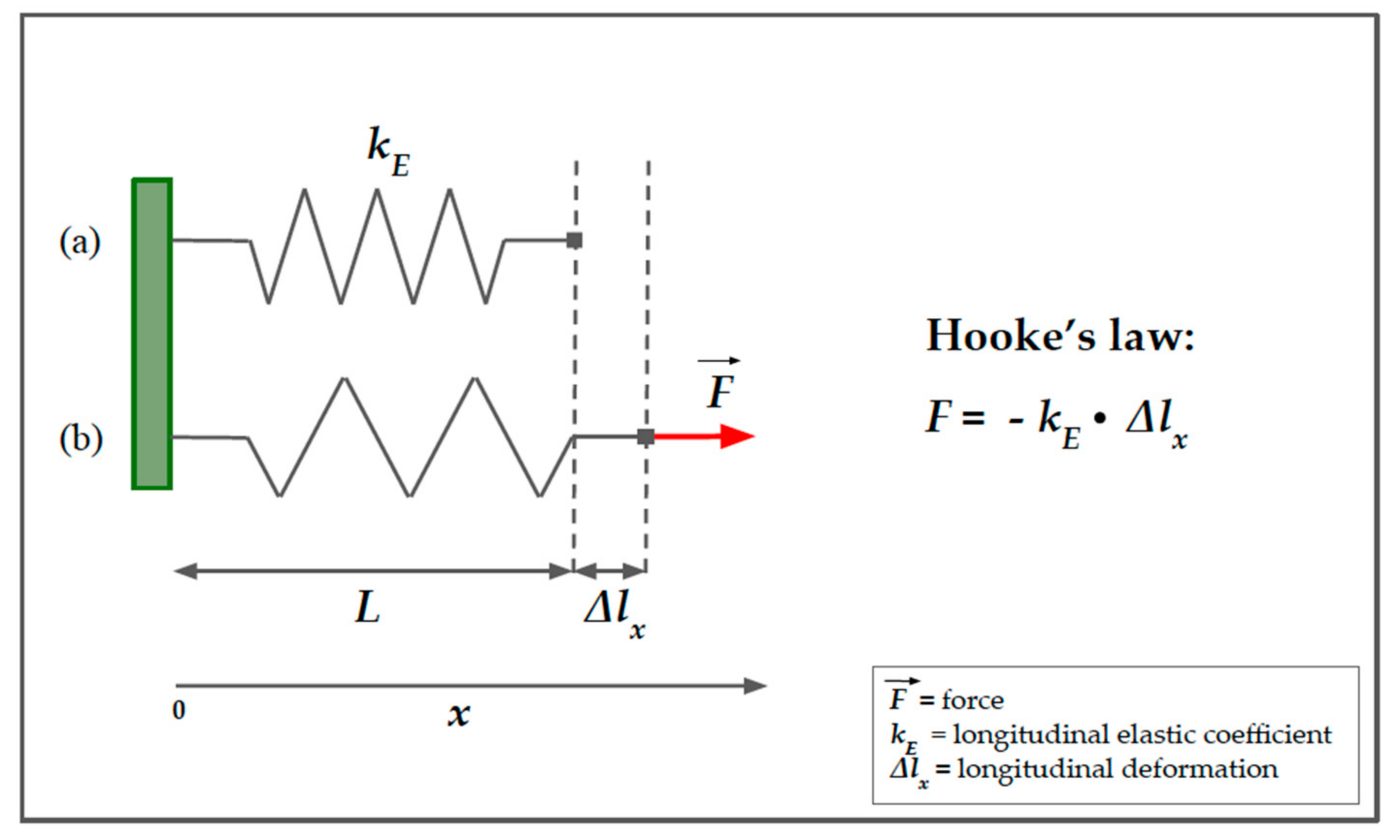
Abstract
:1. Introduction
2. Principles of Ultrasound Elastography
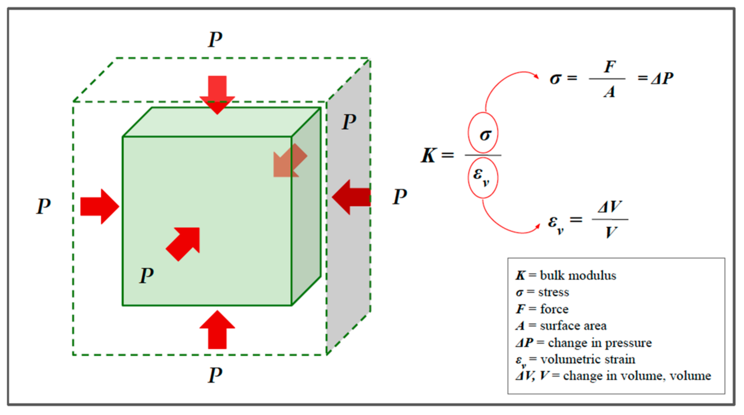
2.1. Definition of Elasticity
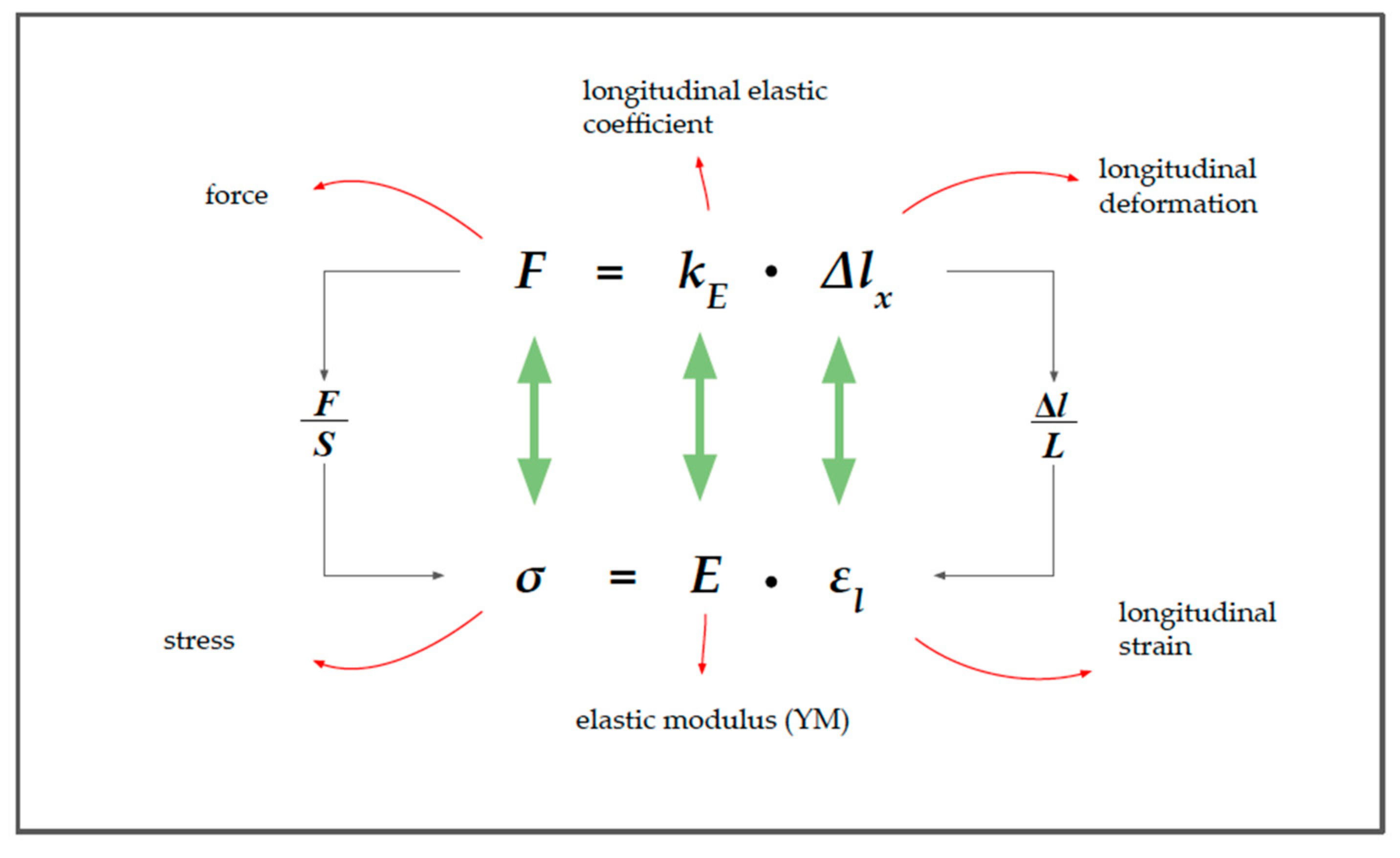
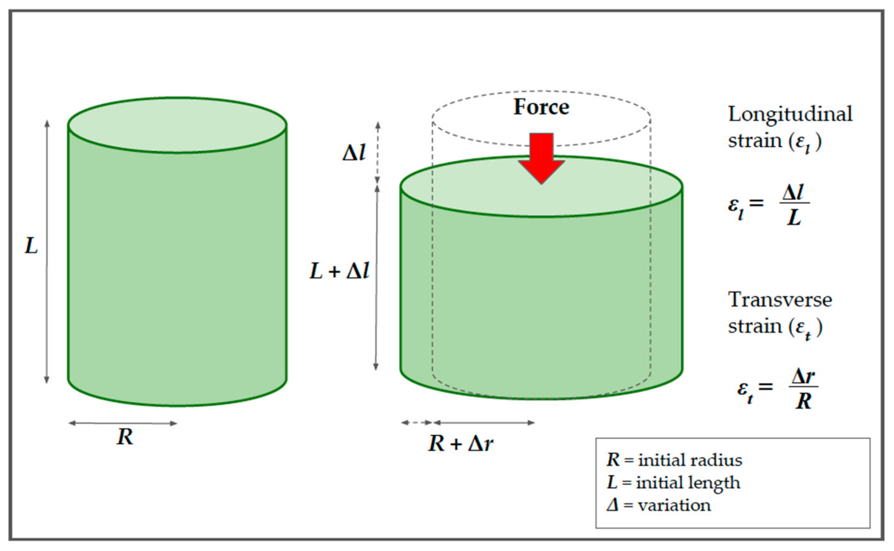
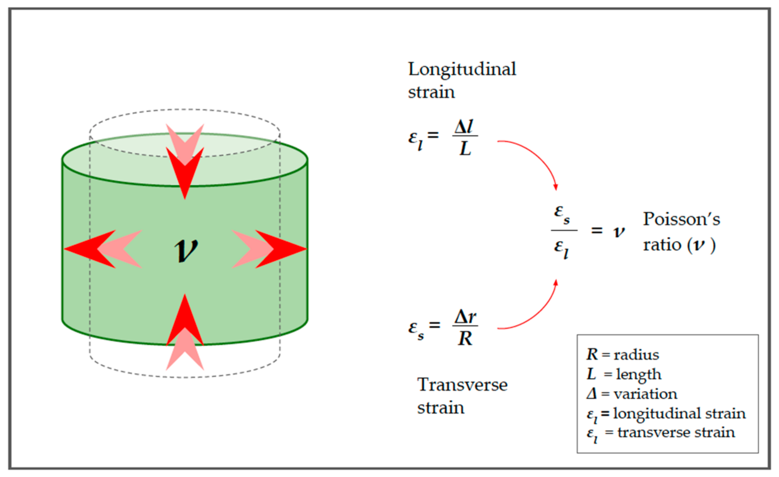
2.2. Longitudinal Elasticity and Young’s Modulus (YM)
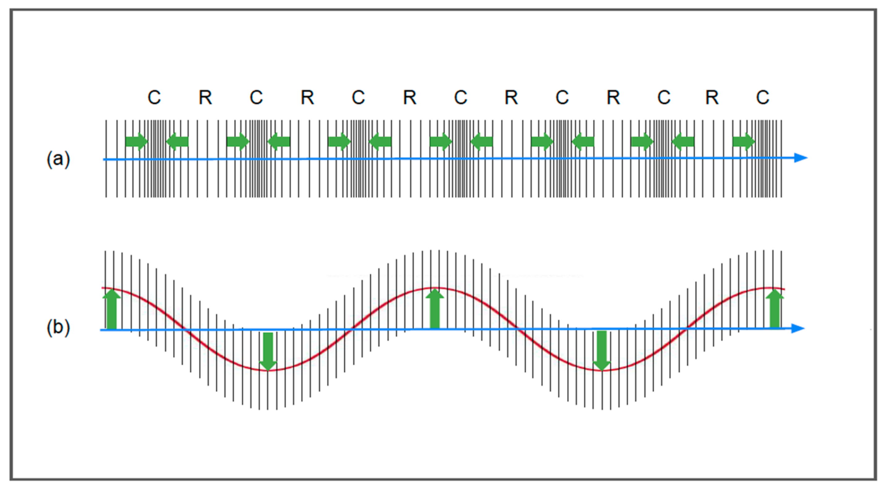
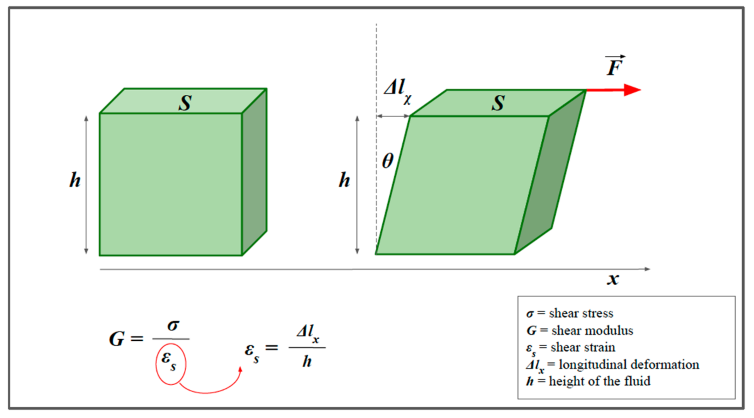
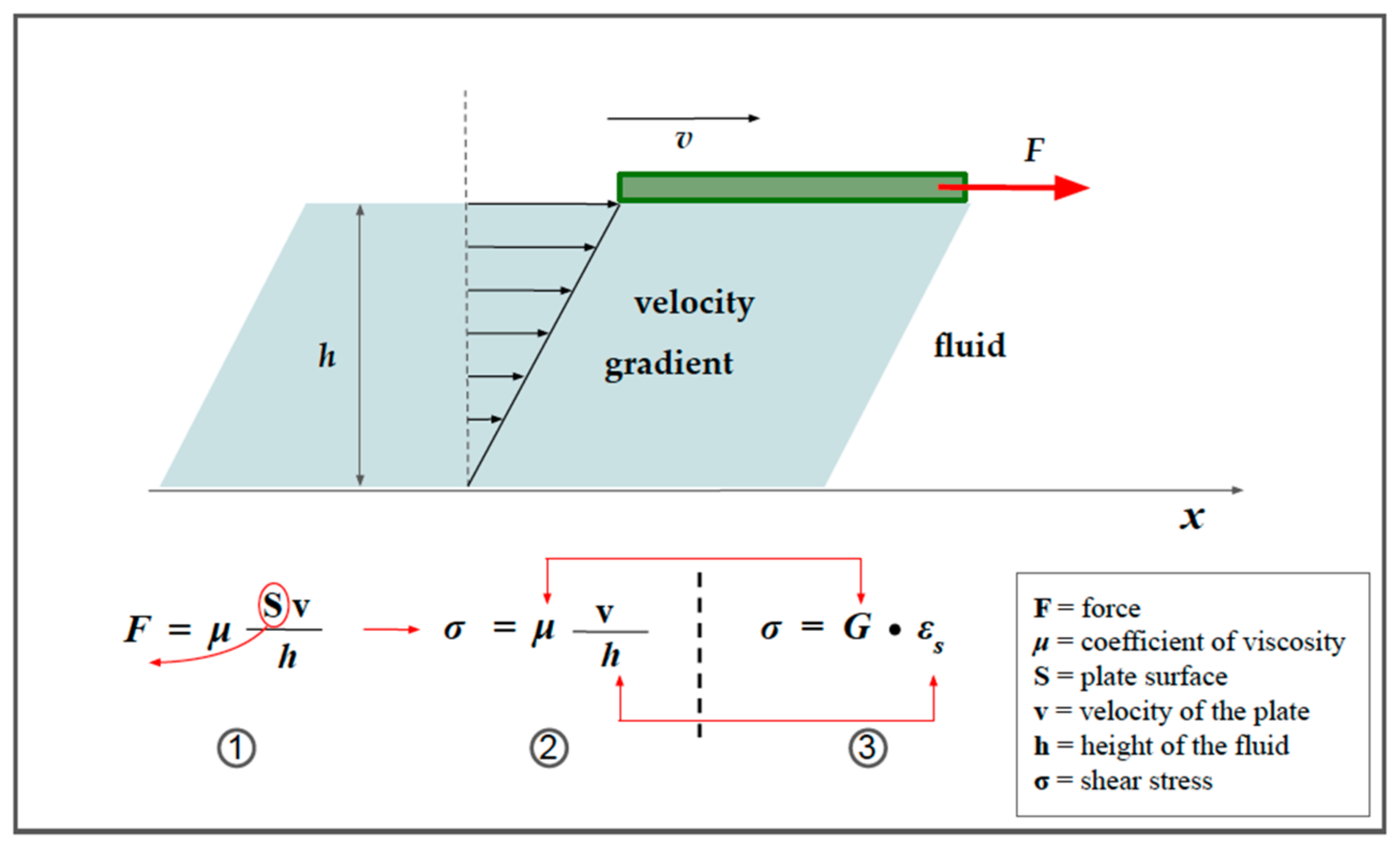
2.3. Shear Wave and Shear Modulus (G)
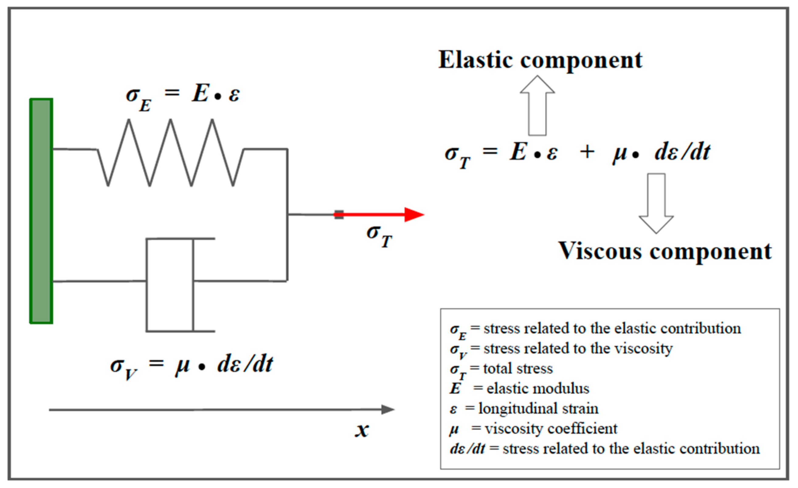
2.4. Viscoelastic Models
3. From Basic Physics to Imaging
3.1. From Elasticity to Strain Imaging
3.2. Visualizing SI information
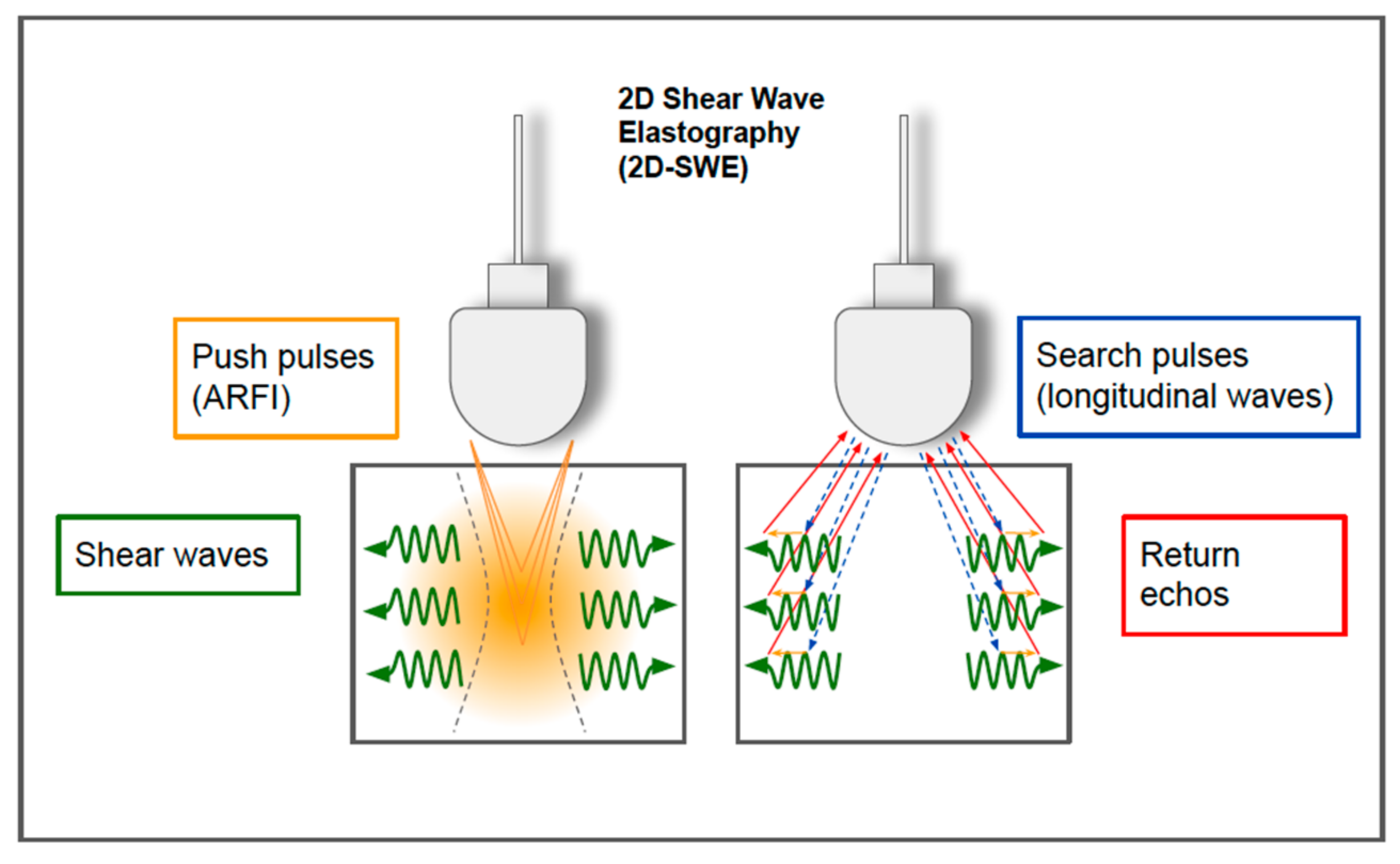
3.3. From Shear Waves to Shear Wave Imaging
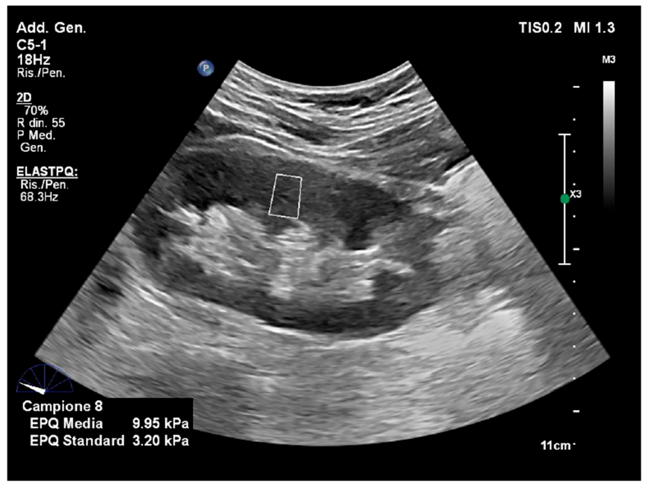
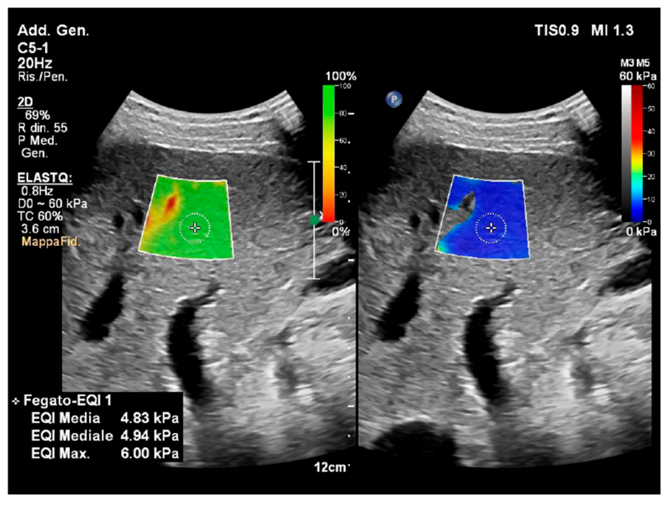
3.4. Visualizing SWE Information
4. Examples of Clinical Applications and Artificial Intelligence Integration
4.1. Liver
4.2. Breast
4.3. Thyroid
4.4. Lymph Nodes
4.5. Bowel
5. Conclusions
Author Contributions
Funding
Institutional Review Board Statement
Informed Consent Statement
Data Availability Statement
Conflicts of Interest
References
- Parker, K.J.; Taylor, L.S.; Gracewski, S.; Rubens, D.J. A unified view of imaging the elastic properties of tissue. J. Acoust. Soc. Am. 2005, 117, 2705–2712. [Google Scholar] [CrossRef] [PubMed]
- Akhtar, R.; Sherratt, M.J.; Cruickshank, J.K.; Derby, B. Characterizing the elastic properties of tissues. Mater. Today 2011, 14, 96–105. [Google Scholar] [CrossRef] [PubMed]
- Ding, Y.; Sun, C.; Zhou, Q.; Cheng, C.; Yan, C.; Wang, B. Use of Palpation Imaging in Diagnosis of Breast Diseases: A Way to Improve the Detection Rate. Med. Sci. Monit. 2020, 26, e927553-1–e927553-10. [Google Scholar] [CrossRef] [PubMed]
- Bamber, J.C. Ultrasound elasticity imaging: Definition and technology. Eur. Radiol. 1999, 9 (Suppl. 3), S327–S330. [Google Scholar] [CrossRef] [PubMed]
- Shiina, T.; Nightingale, K.R.; Palmeri, M.L.; Hall, T.J.; Bamber, J.C.; Barr, R.G.; Castera, L.; Choi, B.I.; Chou, Y.-H.; Cosgrove, D.; et al. WFUMB Guidelines and Recommendations for Clinical Use of Ultrasound Elastography: Part 1: Basic Principles and Terminology. Ultrasound Med. Biol. 2015, 41, 1126–1147. [Google Scholar] [CrossRef] [Green Version]
- Hill, C.R.; Bamber, J.C.; ter Haar, G.R. (Eds.) Physical Principles of Medical Ultrasonics; John Wiley: Chichester, UK, 2004. [Google Scholar]
- Sigrist, R.M.S.; Liau, J.; Kaffas, A.E.; Chammas, M.C.; Willmann, J.K. Ultrasound Elastography: Review of Techniques and Clinical Applications. Theranostics 2017, 7, 1303–1329. [Google Scholar] [CrossRef]
- Ozturk, A.; Grajo, J.R.; Dhyani, M.; Anthony, B.W.; Samir, A.E. Principles of ultrasound elastography. Abdom. Radiol. 2018, 43, 773–785. [Google Scholar] [CrossRef]
- Kwon, S.J.; Jeong, M.K. Advances in ultrasound elasticity imaging. Biomed. Eng. Lett. 2017, 7, 71–79. [Google Scholar] [CrossRef]
- Wells, P.N.T.; Liang, H.-D. Medical ultrasound: Imaging of soft tissue strain and elasticity. J. R. Soc. Interface 2011, 8, 1521–1549. [Google Scholar] [CrossRef] [Green Version]
- Li, G.-Y.; Cao, Y. Mechanics of ultrasound elastography. Proc. R. Soc. A Math. Phys. Eng. Sci. 2017, 473, 20160841. [Google Scholar] [CrossRef]
- Greenleaf, J.F.; Fatemi, M.; Insana, M. Selected Methods for Imaging Elastic Properties of Biological Tissues. Annu. Rev. Biomed. Eng. 2003, 5, 57–78. [Google Scholar] [CrossRef] [Green Version]
- Halliday, D.; Resnik, R.; Krane, K.S. Physics, 5th ed.; John Wiley: Hoboken, NJ, USA, 2001; Volume 1. [Google Scholar]
- Callister, W.D. Materials Science and Engineering: An Introduction, 2nd ed.; Wiley: New York, NY, USA, 2000. [Google Scholar]
- Zheng, Y.; Zheng, Y.; Chen, X.; Yao, A.; Lin, H.; Shen, Y.; Zhu, Y.; Lu, M.; Wang, T.; Chen, S. (Eds.) Shear Wave Propagation in Soft Tissue and Ultrasound Vibrometry. In Wave Propagation Theories and Applications; IntechOpen: London, UK, 2013. [Google Scholar] [CrossRef] [Green Version]
- Deffieux, T.; Montaldo, G.; Tanter, M.; Fink, M. Shear Wave Spectroscopy for In Vivo Quantification of Human Soft Tissues Visco-Elasticity. IEEE Trans. Med. Imaging 2009, 28, 313–322. [Google Scholar] [CrossRef]
- Chen, S.; Fatemi, M.; Greenleaf, J.F. Quantifying elasticity and viscosity from measurement of shear wave speed dispersion. J. Acoust. Soc. Am. 2004, 115, 2781–2785. [Google Scholar] [CrossRef]
- Ophir, J.; Céspedes, I.; Ponnekanti, H.; Yazdi, Y.; Li, X. Elastography: A Quantitative Method for Imaging the Elasticity of Biological Tissues. Ultrason. Imaging 1991, 13, 111–134. [Google Scholar] [CrossRef]
- Hall, T.J.; Zhu, Y.; Spalding, C.S. In vivo real-time freehand palpation imaging. Ultrasound Med. Biol. 2003, 29, 427–435. [Google Scholar] [CrossRef]
- Nightingale, K.R.; Palmeri, M.L.; Nightingale, R.W.; Trahey, G.E. On the feasibility of remote palpation using acoustic radiation force. J. Acoust. Soc. Am. 2001, 110, 625–634. [Google Scholar] [CrossRef]
- Nightingale, K.; Soo, M.S.; Nightingale, R.; Trahey, G. Acoustic radiation force impulse imaging: In vivo demonstration of clinical feasibility. Ultrasound Med. Biol. 2002, 28, 227–235. [Google Scholar] [CrossRef]
- Doherty, J.R.; Trahey, G.E.; Nightingale, K.R.; Palmeri, M.L. Acoustic radiation force elasticity imaging in diagnostic ultrasound. IEEE Trans. Ultrason. Ferroelectr. Freq. Control 2013, 60, 685–701. [Google Scholar] [CrossRef]
- Dietrich, C.F.; Barr, R.G.; Farrokh, A.; Dighe, M.; Hocke, M.; Jenssen, C.; Dong, Y.; Saftoiu, A.; Havre, R.F. Strain Elastography—How To Do It? Ultrasound Int. Open 2017, 3, E137–E149. [Google Scholar] [CrossRef]
- Shiina, T.; Nitta, N.; Ueno, E.; Bamber, J.C. Real time tissue elasticity imaging using the combined autocorrelation method. J. Med. Ultrason. 2002, 29, 119–128. [Google Scholar] [CrossRef]
- Garra, B.S.; Cespedes, E.I.; Ophir, J.; Spratt, S.R.; Zuurbier, R.A.; Magnant, C.M.; Pennanen, M.F. Elastography of breast lesions: Initial clinical results. Radiology 1997, 202, 79–86. [Google Scholar] [CrossRef] [PubMed]
- Gennisson, J.-L.; Deffieux, T.; Fink, M.; Tanter, M. Ultrasound elastography: Principles and techniques. Diagn. Interv. Imaging 2013, 94, 487–495. [Google Scholar] [CrossRef] [PubMed]
- Dobruch-Sobczak, K. The differentiation of the character of solid lesions in the breast in the compression sonoelastography. Part II: Diagnostic value of BIRADS-US classification, Tsukuba score and FLR ratio. J. Ultrason. 2013, 13, 31–49. [Google Scholar] [CrossRef] [PubMed]
- Asteria, C.; Giovanardi, A.; Pizzocaro, A.; Cozzaglio, L.; Morabito, A.; Somalvico, F.; Zoppo, A. US-Elastography in the Differential Diagnosis of Benign and Malignant Thyroid Nodules. Thyroid 2008, 18, 523–531. [Google Scholar] [CrossRef]
- Rago, T.; Santini, F.; Scutari, M.; Pinchera, A.; Vitti, P. Elastography: New Developments in Ultrasound for Predicting Malignancy in Thyroid Nodules. J. Clin. Endocrinol. Metab. 2007, 92, 2917–2922. [Google Scholar] [CrossRef] [Green Version]
- Sconfienza, L.M.; Cavallaro, F.; Colombi, V.; Pastorelli, L.; Tontini, G.; Pescatori, L.; Esseridou, A.; Savarino, E.; Messina, C.; Casale, R.; et al. In-vivo Axial-strain Sonoelastography Helps Distinguish Acutely-inflamed from Fibrotic Terminal Ileum Strictures in Patients with Crohn’s Disease: Preliminary Results. Ultrasound Med. Biol. 2016, 42, 855–863. [Google Scholar] [CrossRef]
- Zhou, J.; Zhou, C.; Zhan, W.; Jia, X.; Dong, Y.; Yang, Z. Elastography ultrasound for breast lesions: Fat-to-lesion strain ratio vs gland-to-lesion strain ratio. Eur. Radiol. 2014, 24, 3171–3177. [Google Scholar] [CrossRef]
- Barr, R.G. Real-time ultrasound elasticity of the breast: Initial clinical results. Ultrasound Q. 2010, 26, 61–66. [Google Scholar] [CrossRef]
- GE Engineering. 2D Shear Wave Elastography LOGIQ E9/E10/E10s. Uploaded on March 2020. Available online: https://ge-ultrasound.eu/wp-content/uploads/2021/02/1.-LOGIQ-E9-LOGIQ-E10-LOGIQ-E10s_Shear-Wave-Whitepaper_2020_JB29031XX.pdf (accessed on 15 December 2022).
- Sandrin, L.; Fourquet, B.; Hasquenoph, J.-M.; Yon, S.; Fournier, C.; Mal, F.; Christidis, C.; Ziol, M.; Poulet, B.; Kazemi, F.; et al. Transient elastography: A new noninvasive method for assessment of hepatic fibrosis. Ultrasound Med. Biol. 2003, 29, 1705–1713. [Google Scholar] [CrossRef]
- Jung, K.S.; Kim, S.U. Clinical applications of transient elastography. Clin. Mol. Hepatol. 2012, 18, 163–173. [Google Scholar] [CrossRef]
- Sarvazyan, A.P.; Rudenko, O.V.; Swanson, S.D.; Fowlkes, J.; Emelianov, S.Y. Shear wave elasticity imaging: A new ultrasonic technology of medical diagnostics. Ultrasound Med. Biol. 1998, 24, 1419–1435. [Google Scholar] [CrossRef]
- Taljanovic, M.S.; Gimber, L.H.; Becker, G.W.; Latt, L.D.; Klauser, A.S.; Melville, D.M.; Gao, L.; Witte, R.S. Shear-Wave Elastography: Basic Physics and Musculoskeletal Applications. Radiographics 2017, 37, 855–870. [Google Scholar] [CrossRef] [Green Version]
- Nightingale, K.; McAleavey, S.; Trahey, G. Shear-wave generation using acoustic radiation force: In vivo and ex vivo results. Ultrasound Med. Biol. 2003, 29, 1715–1723. [Google Scholar] [CrossRef]
- Ferraioli, G.; Wong, V.W.-S.; Castera, L.; Berzigotti, A.; Sporea, I.; Dietrich, C.F.; Choi, B.I.; Wilson, S.R.; Kudo, M.; Barr, R.G. Liver Ultrasound Elastography: An Update to the World Federation for Ultrasound in Medicine and Biology Guidelines and Recommendations. Ultrasound Med. Biol. 2018, 44, 2419–2440. [Google Scholar] [CrossRef] [Green Version]
- Barr, R.G.; Wilson, S.R.; Rubens, D.; Garcia-Tsao, G.; Ferraioli, G. Update to the Society of Radiologists in Ultrasound Liver Elastography Consensus Statement. Radiology 2020, 296, 263–274. [Google Scholar] [CrossRef]
- Ferraioli, G.; Filice, C.; Castera, L.; Choi, B.I.; Sporea, I.; Wilson, S.R.; Cosgrove, D.; Dietrich, C.F.; Amy, D.; Bamber, J.C.; et al. WFUMB Guidelines and Recommendations for Clinical Use of Ultrasound Elastography: Part 3: Liver. Ultrasound Med. Biol. 2015, 41, 1161–1179. [Google Scholar] [CrossRef] [Green Version]
- Friedrich-Rust, M.; Nierhoff, J.; Lupsor-Platon, M.; Sporea, I.; Fierbinteanu-Braticevici, C.; Strobel, D.; Takahashi, H.; Yoneda, M.; Suda, T.; Zeuzem, S.; et al. Performance of Acoustic Radiation Force Impulse imaging for the staging of liver fibrosis: A pooled meta-analysis. J. Viral Hepat. 2011, 19, e212–e219. [Google Scholar] [CrossRef]
- Fraquelli, M.; Rigamonti, C.; Casazza, G.; Conte, D.; Donato, M.F.; Ronchi, G.; Colombo, M. Reproducibility of transient elastography in the evaluation of liver fibrosis in patients with chronic liver disease. Gut 2007, 56, 968–973. [Google Scholar] [CrossRef] [Green Version]
- Muthiah, M.D.; Sanyal, A.J. Burden of Disease due to Nonalcoholic Fatty Liver Disease. Gastroenterol. Clin. N. Am. 2020, 49, 1–23. [Google Scholar] [CrossRef]
- Xiao, G.; Zhu, S.; Xiao, X.; Yan, L.; Yang, J.; Wu, G. Comparison of laboratory tests, ultrasound, or magnetic resonance elastography to detect fibrosis in patients with nonalcoholic fatty liver disease: A metaanalysis. Hepatology 2017, 66, 1486–1501. [Google Scholar] [CrossRef] [Green Version]
- Sasso, M.; Beaugrand, M.; de Ledinghen, V.; Douvin, C.; Marcellin, P.; Poupon, R.; Sandrin, L.; Miette, V. Controlled Attenuation Parameter (CAP): A Novel VCTE™ Guided Ultrasonic Attenuation Measurement for the Evaluation of Hepatic Steatosis: Preliminary Study and Validation in a Cohort of Patients with Chronic Liver Disease from Various Causes. Ultrasound Med. Biol. 2010, 36, 1825–1835. [Google Scholar] [CrossRef] [PubMed]
- Cao, Y.-T.; Xiang, L.-L.; Qi, F.; Zhang, Y.-J.; Chen, Y.; Zhou, X.-Q. Accuracy of controlled attenuation parameter (CAP) and liver stiffness measurement (LSM) for assessing steatosis and fibrosis in non-alcoholic fatty liver disease: A systematic review and meta-analysis. Eclinicalmedicine 2022, 51, 101547. [Google Scholar] [CrossRef] [PubMed]
- De Ledinghen, V.; Hiriart, J.B.; Vergniol, J.; Merrouche, W.; Bedossa, P.; Paradis, V. Controlled attenuation parameter (CAP) with the XL probe of the Fibroscan: A comparative study with the M probe and liver biopsy. Dig. Dis. Sci. 2017, 62, 2569–2577. [Google Scholar] [CrossRef] [PubMed]
- Yazaki, T.; Tobita, H.; Sato, S.; Miyake, T.; Kataoka, M.; Ishihara, S. Combinational elastography for assessment of liver fibrosis in patients with liver injury. J. Int. Med. Res. 2022, 50, 3000605221100126. [Google Scholar] [CrossRef] [PubMed]
- Wong, G.L.; Yuen, P.; Ma, A.J.; Chan, A.W.; Leung, H.H.; Wong, V.W. Artificial intelligence in prediction of non-alcoholic fatty liver disease and fibrosis. J. Gastroenterol. Hepatol. 2021, 36, 543–550. [Google Scholar] [CrossRef]
- Wang, K.; Lu, X.; Zhou, H.; Gao, Y.; Zheng, J.; Tong, M.; Wu, C.; Liu, C.; Huang, L.; Jiang, T.; et al. Deep learning Radiomics of shear wave elastography significantly improved diagnostic performance for assessing liver fibrosis in chronic hepatitis B: A prospective multicentre study. Gut 2019, 68, 729–741. [Google Scholar] [CrossRef] [Green Version]
- Destrempes, F.; Gesnik, M.; Chayer, B.; Roy-Cardinal, M.-H.; Olivié, D.; Giard, J.-M.; Sebastiani, G.; Nguyen, B.N.; Cloutier, G.; Tang, A. Quantitative ultrasound, elastography, and machine learning for assessment of steatosis, inflammation, and fibrosis in chronic liver disease. PLoS ONE 2022, 17, e0262291. [Google Scholar] [CrossRef]
- Park, S.-Y.; Kang, B.J. Combination of shear-wave elastography with ultrasonography for detection of breast cancer and reduction of unnecessary biopsies: A systematic review and meta-analysis. Ultrasonography 2021, 40, 318–332. [Google Scholar] [CrossRef]
- Itoh, A.; Ueno, E.; Tohno, E.; Kamma, H.; Takahashi, H.; Shiina, T.; Yamakawa, M.; Matsumura, T. Breast Disease: Clinical Application of US Elastography for Diagnosis. Radiology 2006, 239, 341–350. [Google Scholar] [CrossRef]
- Ueno, E.; Umemoto, T.; Bando, H.; Tohno, E.; Waki, K.; Matsumura, T. New Quantitative Method in Breast Elastography: Fat Lesion Ratio (FLR). In Proceedings of the Radiological Society of North America 2007 Scientific Assembly and Annual Meeting, Chicago, IL, USA, 27 November 2007. [Google Scholar]
- Sadigh, G.; Carlos, R.C.; Neal, C.H.; Dwamena, B.A. Accuracy of quantitative ultrasound elastography for differentiation of malignant and benign breast abnormalities: A meta-analysis. Breast Cancer Res. Treat. 2012, 134, 923–931. [Google Scholar] [CrossRef]
- Ricci, P.; Maggini, E.; Mancuso, E.; Lodise, P.; Cantisani, V.; Catalano, C. Clinical application of breast elastography: State of the art. Eur. J. Radiol. 2014, 83, 429–437. [Google Scholar] [CrossRef]
- Gong, X.; Xu, Q.; Xu, Z.; Xiong, P.; Yan, W.; Chen, Y. Real-time elastography for the differentiation of benign and malignant breast lesions: A meta-analysis. Breast Cancer Res. Treat. 2011, 130, 11–18. [Google Scholar] [CrossRef]
- Li, C.; Li, J.; Tan, T.; Chen, K.; Xu, Y.; Wu, R. Application of ultrasonic dual-mode artificially intelligent architecture in assisting radiologists with different diagnostic levels on breast masses classification. Diagn. Interv. Radiol. 2021, 27, 315–322. [Google Scholar] [CrossRef]
- Kim, M.Y.; Kim, S.-Y.; Kim, Y.S.; Kim, E.S.; Chang, J.M. Added value of deep learning-based computer-aided diagnosis and shear wave elastography to b-mode ultrasound for evaluation of breast masses detected by screening ultrasound. Medicine 2021, 100, e26823. [Google Scholar] [CrossRef]
- Kobaly, K.; Kim, C.S.; Mandel, S.J. Contemporary Management of Thyroid Nodules. Annu. Rev. Med. 2022, 73, 517–528. [Google Scholar] [CrossRef]
- Kant, R.; Davis, A.; Verma, V. Thyroid Nodules: Advances in Evaluation and Management. Am. Fam. Physician 2020, 102, 298–304. [Google Scholar]
- Yoon, J.H.; Kim, E.-K.; Kwak, J.Y.; Moon, H.J. Effectiveness and Limitations of Core Needle Biopsy in the Diagnosis of Thyroid Nodules: Review of Current Literature. J. Pathol. Transl. Med. 2015, 49, 230–235. [Google Scholar] [CrossRef] [Green Version]
- Abou Shaar, B.; Meteb, M.; Awad El-Karim, G.; Almalki, Y. Reducing the Number of Unnecessary Thyroid Nodule Biopsies With the American College of Radiology (ACR) Thyroid Imaging Reporting and Data System (TI-RADS). Cureus 2022, 14, e23118. [Google Scholar] [CrossRef]
- Lyshchik, A.; Higashi, T.; Asato, R.; Tanaka, S.; Ito, J.; Mai, J.J.; Pellot-Barakat, C.; Insana, M.F.; Brill, A.B.; Saga, T.; et al. Thyroid Gland Tumor Diagnosis at US Elastography. Radiology 2005, 237, 202–211. [Google Scholar] [CrossRef] [Green Version]
- Azizi, G.; Keller, J.; Lewis, M.; Puett, D.; Rivenbark, K.; Malchoff, C. Performance of Elastography for the Evaluation of Thyroid Nodules: A Prospective Study. Thyroid 2013, 23, 734–740. [Google Scholar] [CrossRef]
- Trimboli, P.; Guglielmi, R.; Monti, S.; Misischi, I.; Graziano, F.; Nasrollah, N.; Amendola, S.; Morgante, S.N.; Deiana, M.G.; Valabrega, S.; et al. Ultrasound Sensitivity for Thyroid Malignancy Is Increased by Real-Time Elastography: A Prospective Multicenter Study. J. Clin. Endocrinol. Metab. 2012, 97, 4524–4530. [Google Scholar] [CrossRef] [PubMed] [Green Version]
- Moon, H.J.; Sung, J.M.; Kim, E.-K.; Yoon, J.H.; Youk, J.H.; Kwak, J.Y. Diagnostic Performance of Gray-Scale US and Elastography in Solid Thyroid Nodules. Radiology 2012, 262, 1002–1013. [Google Scholar] [CrossRef] [PubMed] [Green Version]
- Hairu, L.; Yulan, P.; Yan, W.; Hong, A.; Xiaodong, Z.; Lichun, Y.; Kun, Y.; Ying, X.; Lisha, L.; Baoming, L.; et al. Elastography for the diagnosis of high-suspicion thyroid nodules based on the 2015 American Thyroid Association guidelines: A multicenter study. BMC Endocr. Disord. 2020, 20, 1–10. [Google Scholar] [CrossRef] [PubMed] [Green Version]
- Zhan, J.; Jin, J.-M.; Diao, X.-H.; Chen, Y. Acoustic radiation force impulse imaging (ARFI) for differentiation of benign and malignant thyroid nodules—A meta-analysis. Eur. J. Radiol. 2015, 84, 2181–2186. [Google Scholar] [CrossRef] [PubMed]
- Lin, P.; Chen, M.; Liu, B.; Wang, S.; Li, X. Diagnostic performance of shear wave elastography in the identification of malignant thyroid nodules: A meta-analysis. Eur. Radiol. 2014, 24, 2729–2738. [Google Scholar] [CrossRef]
- Bardet, S.; Ciappuccini, R.; Pellot-Barakat, C.; Monpeyssen, H.; Michels, J.-J.; Tissier, F.; Blanchard, D.; Menegaux, F.; De Raucourt, D.; Lefort, M.; et al. Shear Wave Elastography in Thyroid Nodules with Indeterminate Cytology: Results of a Prospective Bicentric Study. Thyroid 2017, 27, 1441–1449. [Google Scholar] [CrossRef]
- Swan, K.Z.; Bonnema, S.J.; Jespersen, M.L.; Nielsen, V.E. Reappraisal of shear wave elastography as a diagnostic tool for identifying thyroid carcinoma. Endocr. Connect. 2019, 8, 1195–1205. [Google Scholar] [CrossRef] [Green Version]
- Swan, K.Z.; Nielsen, V.E.; Bonnema, S.J. Evaluation of thyroid nodules by shear wave elastography: A review of current knowledge. J. Endocrinol. Investig. 2021, 44, 2043–2056. [Google Scholar] [CrossRef]
- Park, A.Y.; Son, E.J.; Han, K.; Youk, J.H.; Kim, J.-A.; Park, C.S. Shear wave elastography of thyroid nodules for the prediction of malignancy in a large scale study. Eur. J. Radiol. 2015, 84, 407–412. [Google Scholar] [CrossRef]
- Han, R.-J.; Du, J.; Li, F.-H.; Zong, H.-R.; Wang, J.-D.; Shen, Y.-L.; Zhou, Q.-Y. Comparisons and Combined Application of Two-Dimensional and Three-Dimensional Real-time Shear Wave Elastography in Diagnosis of Thyroid Nodules. J. Cancer 2019, 10, 1975–1984. [Google Scholar] [CrossRef]
- Petersen, M.; Schenke, S.A.; Firla, J.; Croner, R.S.; Kreissl, M.C. Shear Wave Elastography and Thyroid Imaging Reporting and Data System (TIRADS) for the Risk Stratification of Thyroid Nodules—Results of a Prospective Study. Diagnostics 2022, 12, 109. [Google Scholar] [CrossRef]
- Filho, R.H.C.; Pereira, F.L.; Iared, W. Diagnostic Accuracy Evaluation of Two-Dimensional Shear Wave Elastography in the Differentiation Between Benign and Malignant Thyroid Nodules. J. Ultrasound Med. 2020, 39, 1729–1741. [Google Scholar] [CrossRef]
- Zhang, B.; Tian, J.; Pei, S.; Chen, Y.; He, X.; Dong, Y.; Zhang, L.; Mo, X.; Huang, W.; Cong, S.; et al. Machine Learning–Assisted System for Thyroid Nodule Diagnosis. Thyroid 2019, 29, 858–867. [Google Scholar] [CrossRef]
- Qin, P.; Wu, K.; Hu, Y.; Zeng, J.; Chai, X. Diagnosis of Benign and Malignant Thyroid Nodules Using Combined Conventional Ultrasound and Ultrasound Elasticity Imaging. IEEE J. Biomed. Health Inform. 2020, 24, 1028–1036. [Google Scholar] [CrossRef]
- Zhao, C.-K.; Ren, T.-T.; Yin, Y.-F.; Shi, H.; Wang, H.-X.; Zhou, B.-Y.; Wang, X.-R.; Li, X.; Zhang, Y.-F.; Liu, C.; et al. A Comparative Analysis of Two Machine Learning-Based Diagnostic Patterns with Thyroid Imaging Reporting and Data System for Thyroid Nodules: Diagnostic Performance and Unnecessary Biopsy Rate. Thyroid 2021, 31, 470–481. [Google Scholar] [CrossRef]
- Liu, T.; Ge, X.; Yu, J.; Guo, Y.; Wang, Y.; Wang, W.; Cui, L. Comparison of the application of B-mode and strain elastography ultrasound in the estimation of lymph node metastasis of papillary thyroid carcinoma based on a radiomics approach. Int. J. Comput. Assist. Radiol. Surg. 2018, 13, 1617–1627. [Google Scholar] [CrossRef]
- Wang, B.; Guo, Q.; Wang, J.-Y.; Yu, Y.; Yi, A.-J.; Cui, X.-W.; Dietrich, C.F. Ultrasound Elastography for the Evaluation of Lymph Nodes. Front. Oncol. 2021, 11, 714660. [Google Scholar] [CrossRef]
- Knabe, M.; Günter, E.; Ell, C.; Pech, O. Can EUS Elastography Improve Lymph Node Staging in Esophageal Cancer? Surg. Endosc. 2013, 27, 1196–1202. [Google Scholar] [CrossRef]
- Tahmasebi, A.; Qu, E.; Sevrukov, A.; Liu, J.-B.; Wang, S.; Lyshchik, A.; Yu, J.; Eisenbrey, J.R. Assessment of Axillary Lymph Nodes for Metastasis on Ultrasound Using Artificial Intelligence. Ultrason. Imaging 2021, 43, 329–336. [Google Scholar] [CrossRef]
- Huang, X.; Zhang, Y.; Du, H.; Lai, L.; Chen, J.; Zhang, T.; Mao, H. Machine Learning-Based Shear Wave Elastography Elastic Index (SWEEI) in Predicting Cervical Lymph Node Metastasis of Papillary Thyroid Microcarcinoma: A Comparative Analysis of Five Practical Prediction Models. Cancer Manag. Res. 2022, 14, 2847–2858. [Google Scholar] [CrossRef]
- Ng, S.C.; Shi, H.Y.; Hamidi, N.; Underwood, F.E.; Tang, W.; Benchimol, E.I.; Panaccione, R.; Ghosh, S.; Wu, J.C.Y.; Chan, F.K.L.; et al. Worldwide incidence and prevalence of inflammatory bowel disease in the 21st century: A systematic review of population-based studies. Lancet 2018, 390, 2769–2778. [Google Scholar] [CrossRef] [PubMed]
- Actis, G.C.; Pellicano, R.; Fagoonee, S.; Ribaldone, D.G. History of Inflammatory Bowel Diseases. J. Clin. Med. 2019, 8, 1970. [Google Scholar] [CrossRef] [PubMed] [Green Version]
- Rodrigues, B.L.; Mazzaro, M.C.; Nagasako, C.K.; Ayrizono, M.D.L.S.; Fagundes, J.J.; Leal, R.F. Assessment of disease activity in inflammatory bowel diseases: Non-invasive biomarkers and endoscopic scores. World J. Gastrointest. Endosc. 2020, 12, 504–520. [Google Scholar] [CrossRef] [PubMed]
- Ślósarz, D.; Poniewierka, E.; Neubauer, K.; Kempiński, R. Ultrasound Elastography in the Assessment of the Intestinal Changes in Inflammatory Bowel Disease—Systematic Review. J. Clin. Med. 2021, 10, 4044. [Google Scholar] [CrossRef] [PubMed]
- Grażyńska, A.; Kufel, J.; Dudek, A.; Cebula, M. Shear Wave and Strain Elastography in Crohn’s Disease—A Systematic Review. Diagnostics 2021, 11, 1609. [Google Scholar] [CrossRef] [PubMed]
- Cebula, M.; Kufel, J.; Grażyńska, A.; Habas, J.; Gruszczyńska, K. Intestinal Elastography in the Diagnostics of Ulcerative Colitis: A Narrative Review. Diagnostics 2022, 12, 2070. [Google Scholar] [CrossRef]
- Alfredsson, J.; Wick, M.J. Mechanism of fibrosis and stricture formation in Crohn’s disease. Scand. J. Immunol. 2020, 92, e12990. [Google Scholar] [CrossRef]
- Zhang, Y.N.; Fowler, K.J.; Ozturk, A.; Bs, C.K.P.; Ba, A.L.L.; Montes, V.; Ba, W.C.H.; Wang, K.; Andre, M.P.; Samir, A.E.; et al. Liver fibrosis imaging: A clinical review of ultrasound and magnetic resonance elastography. J. Magn. Reson. Imaging 2020, 51, 25–42. [Google Scholar] [CrossRef]
- Re, G.L.; Picone, D.; Vernuccio, F.; Scopelliti, L.; Di Piazza, A.; Tudisca, C.; Serraino, S.; Privitera, G.; Midiri, F.; Salerno, S.; et al. Comparison of US Strain Elastography and Entero-MRI to Typify the Mesenteric and Bowel Wall Changes during Crohn’s Disease: A Pilot Study. BioMed Res. Int. 2017, 2017, 4257987. [Google Scholar] [CrossRef] [Green Version]
- Fraquelli, M.; Branchi, F.; Cribiù, F.M.; Orlando, S.; Casazza, G.; Magarotto, A.; Massironi, S.; Botti, F.; Contessini-Avesani, E.; Conte, D.; et al. The Role of Ultrasound Elasticity Imaging in Predicting Ileal Fibrosis in Crohnʼs Disease Patients. Inflamm. Bowel Dis. 2015, 21, 2605–2612. [Google Scholar] [CrossRef]
- Serra, C.; Rizzello, F.; Pratico’, C.; Felicani, C.; Fiorini, E.; Brugnera, R.; Mazzotta, E.; Giunchi, F.; Fiorentino, M.; D’Errico, A.; et al. Real-time elastography for the detection of fibrotic and inflammatory tissue in patients with stricturing Crohn’s disease. J. Ultrasound 2017, 20, 273–284. [Google Scholar] [CrossRef]
- Gubatan, J.; Levitte, S.; Patel, A.; Balabanis, T.; Wei, M.T.; Sinha, S.R. Artificial intelligence applications in inflammatory bowel disease: Emerging technologies and future directions. World J. Gastroenterol. 2021, 27, 1920–1935. [Google Scholar] [CrossRef]


Disclaimer/Publisher’s Note: The statements, opinions and data contained in all publications are solely those of the individual author(s) and contributor(s) and not of MDPI and/or the editor(s). MDPI and/or the editor(s) disclaim responsibility for any injury to people or property resulting from any ideas, methods, instructions or products referred to in the content. |
© 2023 by the authors. Licensee MDPI, Basel, Switzerland. This article is an open access article distributed under the terms and conditions of the Creative Commons Attribution (CC BY) license (https://creativecommons.org/licenses/by/4.0/).
Share and Cite
Cè, M.; D'Amico, N.C.; Danesini, G.M.; Foschini, C.; Oliva, G.; Martinenghi, C.; Cellina, M. Ultrasound Elastography: Basic Principles and Examples of Clinical Applications with Artificial Intelligence—A Review. BioMedInformatics 2023, 3, 17-43. https://doi.org/10.3390/biomedinformatics3010002
Cè M, D'Amico NC, Danesini GM, Foschini C, Oliva G, Martinenghi C, Cellina M. Ultrasound Elastography: Basic Principles and Examples of Clinical Applications with Artificial Intelligence—A Review. BioMedInformatics. 2023; 3(1):17-43. https://doi.org/10.3390/biomedinformatics3010002
Chicago/Turabian StyleCè, Maurizio, Natascha Claudia D'Amico, Giulia Maria Danesini, Chiara Foschini, Giancarlo Oliva, Carlo Martinenghi, and Michaela Cellina. 2023. "Ultrasound Elastography: Basic Principles and Examples of Clinical Applications with Artificial Intelligence—A Review" BioMedInformatics 3, no. 1: 17-43. https://doi.org/10.3390/biomedinformatics3010002