Enhancing Explainable Machine Learning by Reconsidering Initially Unselected Items in Feature Selection for Classification

Abstract

Feature selection is a common step in data preprocessing that precedes machine learning to reduce data space and the computational cost of processing or obtaining the data. Filtering out uninformative variables is also important for knowledge discovery. By reducing the data space to only those components that are informative to the class structure, feature selection can simplify models so that they can be more easily interpreted by researchers in the field, reminiscent of explainable artificial intelligence. Knowledge discovery in complex data thus benefits from feature selection that aims to understand feature sets in the thematic context from which the data set originates. However, a single variable selected from a very small number of variables that are technically sufficient for AI training may make little immediate thematic sense, whereas the additional consideration of a variable discarded during feature selection could make scientific discovery very explicit. In this report, we propose an approach to explainable feature selection (XFS) based on a systematic reconsideration of unselected features. The difference between the respective classifications when training the algorithms with the selected features or with the unselected features provides a valid estimate of whether the relevant features in a data set have been selected and uninformative or trivial information was filtered out. It is shown that revisiting originally unselected variables in multivariate data sets allows for the detection of pathologies and errors in the feature selection that occasionally resulted in the failure to identify the most appropriate variables.

1. Introduction

Feature selection (for an overview, see e.g., [1]), is a frequent step of data preprocessing preceding machine-learning to reduce the data space and the computational load to process it, or the costs to acquire relevant data. Feature selection thus filters the information contained in a data set and removes uninformative variables, considering that machine learning algorithms need examples of the relevant structures in an empirical data set. Filtering out uninformative variables is also relevant to knowledge discovery. By reducing the data space to its components informative for the class structure, feature selection can simplify models to make them easier to interpret by field researchers, addressing explainable artificial intelligence (XAI) [2].

Too much information represented in many variables can prevent field experts from grasping the main mechanistic processes underlying a class structure in a data set. This is consistent with an observation more than half a century old that human intelligibility is limited, with a proposed optimum of 7 ± 2 [3]. On the other hand, too few features resulting from rigorous selection may be sufficient for successful classification by the AI, but insufficient for field experts to understand the key processes underlying the structure in the data. For example, of two highly correlated variables, one may be technically better for the AI to function and is therefore selected, but the other would make sense in the context of the actual research topic. Few selected variables may be functioning for an algorithm. However, they may provide a fragmented picture of the underlying process. The additional consideration of variables that were discarded during feature selection could make the scientific result very clear.

Knowledge discovery in complex data thus appears to potentially benefit from feature selection aimed at understandable feature sets in the topical research context from which the data set originates. Knowledge discovery via feature selection for classifiers is based on the idea that if an algorithm can be trained to assign a case to the correct class, the data contains a structure relevant to the class structure, and the variables that the algorithm needs to successfully perform its task are the class-relevant variables or features in the actual data set. However, the interpretation of a feature set in a specific research context may vary depending on whether it can be stated that only the selected features, but not the unselected features, provide a the information necessary for correct class assignment. This would allow the variables not selected to be discarded as uninteresting, and the result of the analysis will be that the process studied is characterized by the variables selected, which may represent scientific progress. For example, if the variables contained genetic information, then the selected features will give a clear indication of the genetic background of the biological process under study. A rigorous feature selection process that provides the minimum amount of information required by an AI for classification might have discarded variables that also provide class-relevant information, only to a lesser extent than the selected variables. In this case, the interpretation of the feature set in the topical context may differ from the one above, i.e., it cannot be claimed that the background mechanisms of the process of interest has been comprehensively captured when interpreting the selected features.

Thus, while usually the interest in the variables omitted during feature selection vanishes, they may still contain relevant information for the topical interpretation unless proven otherwise. Specific attempts on this topic are so far limited, such as highlighting that extracting a subset of the most important features could help researchers understand the biological processes underlying the disease [4]. Therefore, this report shows that classification performance obtained with the unselected features can be used to improve the interpretation of feature sets. The evaluation of classification performance with both the selected and unselected features provides an indication of whether informative features have been left aside. This information can critically affect the interpretation of a feature set if the selection process was conducted with the goal of knowledge discovery. Therefore, this report proposes an explainable feature selection (XFS) approach based on a systematic reconsideration of the unselected features.

2. Methods

2.1. Algorithm

Three criteria are proposed that a set of features should satisfy in order to both capture the background mechanisms of the process in terms of the explainable feature selection (XFS) and to have identified the most appropriate variables for the class assignment.

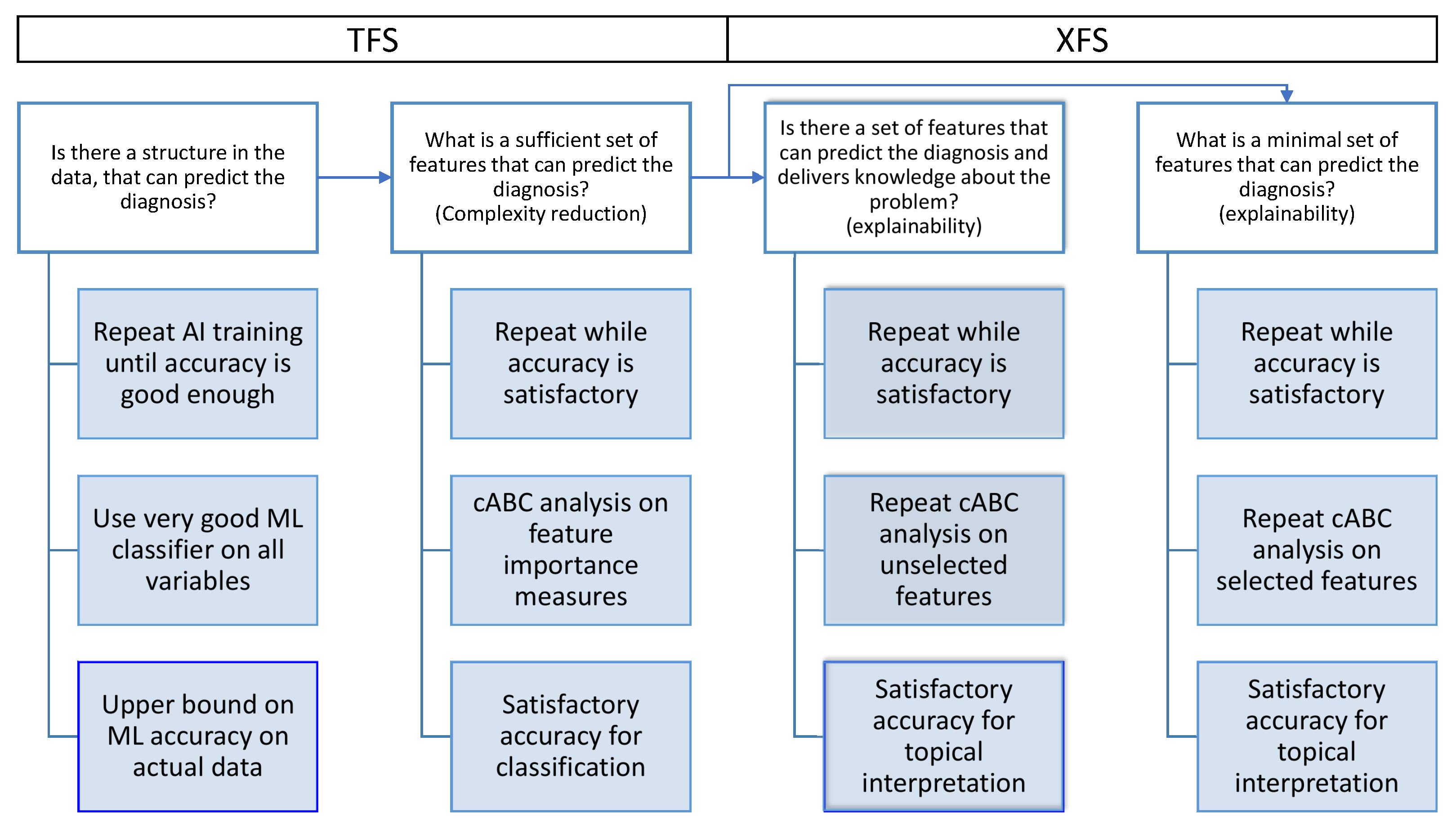
• Classification performance of algorithms trained with the selected features should be satisfactory, which is routinely checked. Ideally, it should not drop significantly from the performance obtained with all features. The classification performance must be at least better than chance, including the lower bound of the 95% confidence interval of classification performance measures, which should be higher than the level of guessing of the class assignment.
• Classification performance with the selected features should be better than classification performance when the training is conducted with the unselected features. This is not routinely checked. The difference between the respective classifications when training the algorithms with the selected features and when training the algorithm with the unselected features should be positive, e.g., with a lower bound of the 95% confidence interval > 0.
• If the difference in point 2 above is not satisfactorily greater than zero, but the classifier trained with the full set of features has satisfactory accuracy, then the unselected features should be reconsidered. If variables are omitted that are very strongly correlated with selected features, an assessment should be triggered of whether correlated variables might add relevant information that improves the (domain expert’s) interpretation of the feature set. In a new feature selection pass, the features already selected from the first pass are omitted. The final feature set is then the union of the two feature sets, provided that the second pass did not fail criterion 1.

2.2. Evaluations

2.2.1. Quantification of Feature Importance

Several different methods of feature selection have been proposed. Overviews on feature selection methods are available in the literature, e.g., [1,5]. Feature selection methods [1] are typically presented in three classes: filter, wrapper and embedded methods. Filter methods suppress the least interesting variables, where interestingness is typically measured as a correlation to the variable to predict [6]. In wrapper methods, subsets of variables are evaluated for an overview, see for example [7]. Ensemble methods try to combine wrapper and filter methods [8]. Implementations include “brute force” approaches limited only by computational power, and various unsupervised and supervised methods. Supervised methods aim at identifying the variable importance via classification performance. Among supervised methods, both univariate and multivariate methods are available in which informative features can be obtained by, for example, recursive feature elimination or sequential feature selection. Particular implementations include the regression-based least absolute shrinkage and selection operators (LASSO [9]), or make use of usually well-performing machine learning methods such as random forests [10,11] and combine them with statistical tests as in the “Boruta” method [12].

Among popular multivariate supervised methods figures selecting features based on the variable importance in random forests classifiers. This can be obtained via permutation weighting [11] from out-of-bag (OOB) cases as the decrease in classification accuracy when the respective feature is omitted from the class assignment, as implemented in the R package “randomForest” (https://cran.r-project.org/package=randomForest (accessed on 3 September 2022) [13]), and callable via “importance=TRUE” in the random forest model constructor and “type=1” in the “importance()” read out function. Of note, the default method of the mentioned R libary, which measures how effective the feature is at reducing theuncertainty when constructing decision trees based on the mean reduction in impurity (or “Gini importance”), was not used because its use has been discouraged, as it has been demonstrated to occasionally produce biased results with inflated importance of numerical features not predictive for unseen data [14,15].

2.2.2. Computation of the Set Size of the Selected Features

Most feature selection methods, including the OOB permutation importance used in the present analyses, do not immediately provide a decision of how many “best” features to select but just a measure of the importance of each feature. Therefore, the size k of the final feature set is often determined arbitrarily.

Typically, feature importance has a highly skewed distribution, i.e., a few variables have high importance, but many have a low importance. This kind of distribution can be addressed with the computed ABC analysis (cABC) [16]. This is an item categorization method that aims to identify the most relevant items by dividing a set of non-negative numeric elements into subsets named “A”, “B” and “C”, such that subset “A” contains the “important few” items while subset “C” contains the “trivial many” items [17]. The algorithmic computation of the set sizes from the data has been described in detail previously [16]. Combining random forests with cABC analysis for feature selection has recently been proposed [18].

2.3. Experimental Setup

Programming was performed in the R language [19] using the R software package [20], version 4.2.1 for Linux, available free of charge from the Comprehensive R Archive Network (CRAN) at https://CRAN.R-project.org/ (accessed on 3 September 2022). Experiments were performed on 1 – 64 cores/threads on an AMD Ryzen Threadripper 3970X (Advanced Micro Devices, Inc., Santa Clara, CA, USA) computer with 256 GB random access memory (RAM) running Ubuntu Linux 22.04.1 LTS (Canonical, London, UK)). The main R packages used for the experiments were “randomForest” (https://cran.r-project.org/package=randomForest (accessed on 3 September 2022) [13]), “caret” (https://cran.r-project.org/package=caret (accessed on 3 September 2022) [21] and our package “ABCanalysis” (https://cran.r-project.org/package=ABCanalysis, (accessed on 3 September 2022) [16]). The computational requirements could be met by parallel processing using the “parallel” library included in the R base environment.

Twenty percent of the original data was separated as a validation data set, which was not further touched during feature selection. To obtain a representative subsample, our R package “opdisDownsampling” (https://cran.r-project.org/package=opdisDownsampling (accessed on 3 September 2022)) was used for this task. The package selects from 10,000–100,000 random samples the one in which the distributions of the variables are most similar to those of the original data. The details of this sampling procedure have been described previously [22].

Random forests were tuned with respect to hyperparameters, as reported previously [23], in order to ensure that the performance of the classifier during feature selection and classification was optimized for the actual data sets. Specifically, tuning was performed via a grid search and using a 100-fold cross-validation precluding each feature selection run. For example, tuning the hyperparameters indicated that for the iris data set (see next chapter) the classifier should be run with $n_{tree}=1100$ trees, $\sqrt{n_{variables}}=2$ features per tree and nodesize = 4. For the wine properties data set (see next chapter), the respective hyperparameter settings were $n_{tree}=100$, $n_{variables}=1$, nodesize = 1.

All feature selection experiments were performed in a 1,000 cross-validation scenario. In each run, from the 80% of the full data sets available for this task after having separated the 20% validation sample (see above), 2/3 were randomly drawn as training data subset using Monte Carlo resampling [24] implemented in the R library “sampling” (https://cran.r-project.org/package=sampling (accessed on 3 September 2022) [25]). The permutation variable importance was calculated directly using the OOB samples created during training with these 2/3 randomly drawn cases.

After feature selection, classification performance was evaluated after training random forests with 2/3 randomly drawn cases from the 80% of the data using only the selected or unselected features, and classification performance was tested with random samples of 80% of the 20% validation sample that were not touched during feature selection or classifier training. Classification performance was measured using balanced accuracy [26] implemented in the R library “caret”.

2.4. Data Sets

2.4.1. Iris Flower Data Example

The iris flower data set set [27,28] contains measurements of the four variables, sepal length and width or petal length and width in centimeters, for 50 flowers of each of the three species, Iris setosa, versicolor, and virginica, providing a 150 × 4 data matrix. The data set was expanded by repeating variables to obtain very strongly correlated variables, or by adding variables as their permuted versions to obtain nonsense variables or by adding trivial information using the class information as the variable. Previous analyses indicated that petal dimensions were the most informative for species separation [29].

2.4.2. Wine Quality Data Set

A second data set was a wine data set from https://www.kaggle.com/datasets/shelvigarg/wine-quality-dataset (accessed 2 November 2022). It contains physicochemical properties of a collection of white and red wines and consists of 4898 samples of white wine and 1599 samples of red wine. Eleven variables on chemical properties are solid acidity, volatile acidity, citric acidity, residual sugar, chlorides, free sulfur dioxide, total sulfur dioxide, density, pH, sulfates, and alcohol. A 12th variable, quality, contains the median of at least three ratings from wine experts who ranked the wine quality of each sample between 0 (very poor) and 10 (very good). The wine data set was used for method development in feature selection for regression problems [30,31]. This provided the relevant features to be identified in the present analysis. Fuzzy techniques were used to identify the variables that had the greatest causal relationship with wine quality: Alcohol, fixed acidity, free sulfur dioxide, residual sugar and volatile acidity, while citric acid and sulfates were also variables that show a causal relationship with wine quality, but not in the same strength as the previous ones [31]. For the present experiments, the regression problem with the normally distributed wine quality variable was transferred into a classification problem via a median split into “low” and “high” quality wines.

3. Results

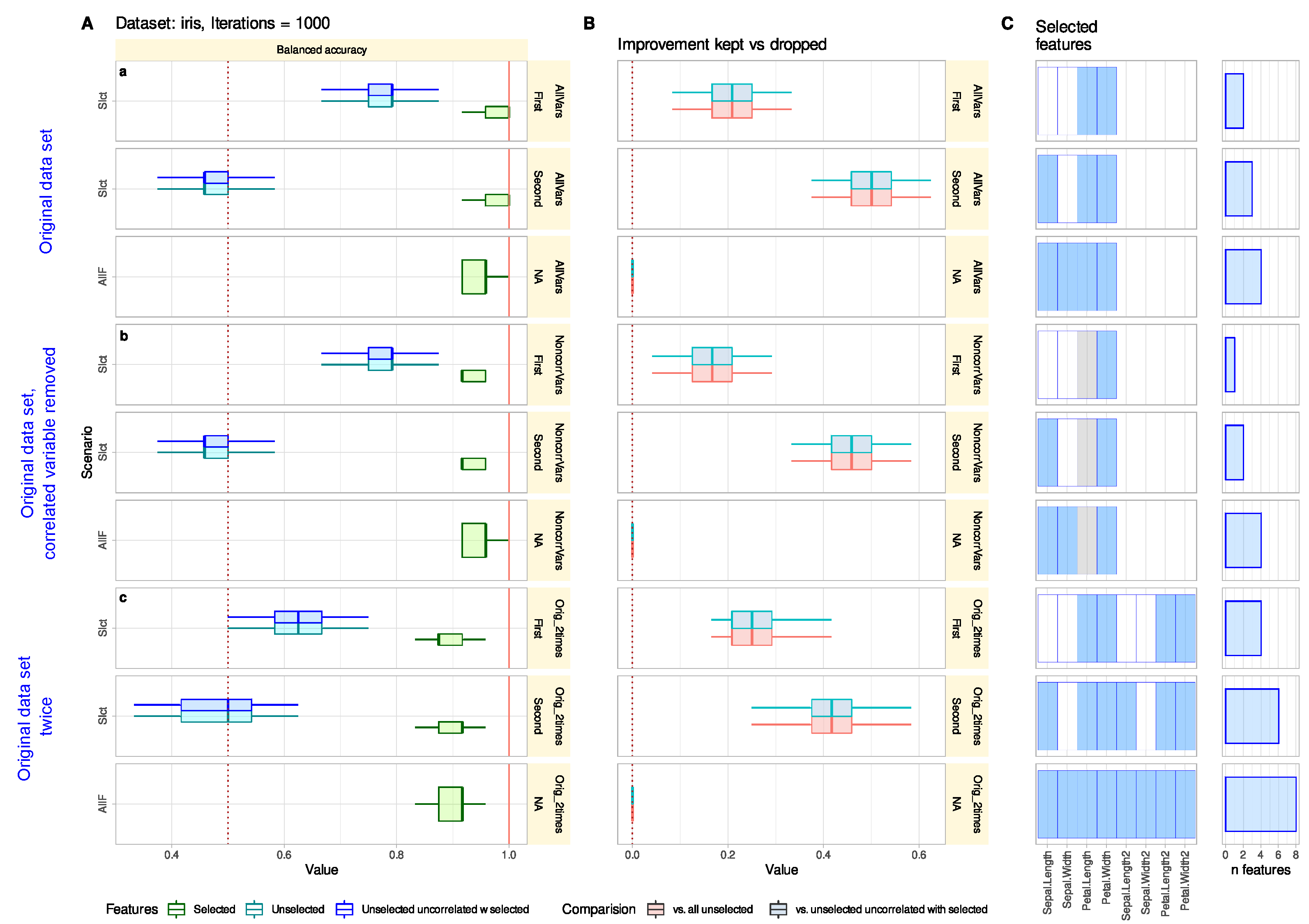
3.1. Iris Flower Data Set

Several modifications of the iris data set were assessed, including (i) the omission of very strongly correlated variables, (ii) the addition of more variables that are perfectly correlated with the existing variables, (iii) the addition of nonsense variables, (iv) the addition of perfect class discriminators, i.e., of the class membership as a variable. Experiments using these modifications allowed for four main conclusions, which are highlighted under the following subheadings.

3.1.1. Default Feature Selection Often Suffices and Removing Strongly Correlated Variables Is Not Necessary

In the iris data set, feature selection identified the two petal dimensions as the most informative for the training of a random forests classifier (Figure 1A(a–c)). Training with these two variables allowed the algorithm to classify the validation data set better than training with the unselected features, i.e., sepal dimensions, as indicated by the 95% confidence interval of the differences in the balanced accuracy located to the right of the zero difference. The median classification performance was even slightly better than when all variables were used for training. Reconsidering the unselected variables in a second round of feature selection added the sepal length to the set of selected features. However, the positive difference in classification performance between selected and unselected features had already indicated that this was unnecessary, and indeed the now larger feature set did not provide a better basis for training the classifier than the two variables selected first.

The petal dimensions were correlated very strongly [32] at a rank correlation [33] coefficient of $\rho$ > 0.9. Petal width was selected as their prototype. In the feature selection among the remaining three variables (Figure 1), it was selected in the first round, while sepal length was added in a second round. However, both sets provided a poorer basis for random forest training than the sets obtained from the full data set without the removal of very strongly correlated variables (see above). The balanced accuracy of the class assignment was not better than with the full data set. When the four variables of the iris data set were added again to the data set (Figure 1 feature selection among the now eight variables remained unaffected and consistent by first referring to the petal dimensions and adding the sepal length in a second round.

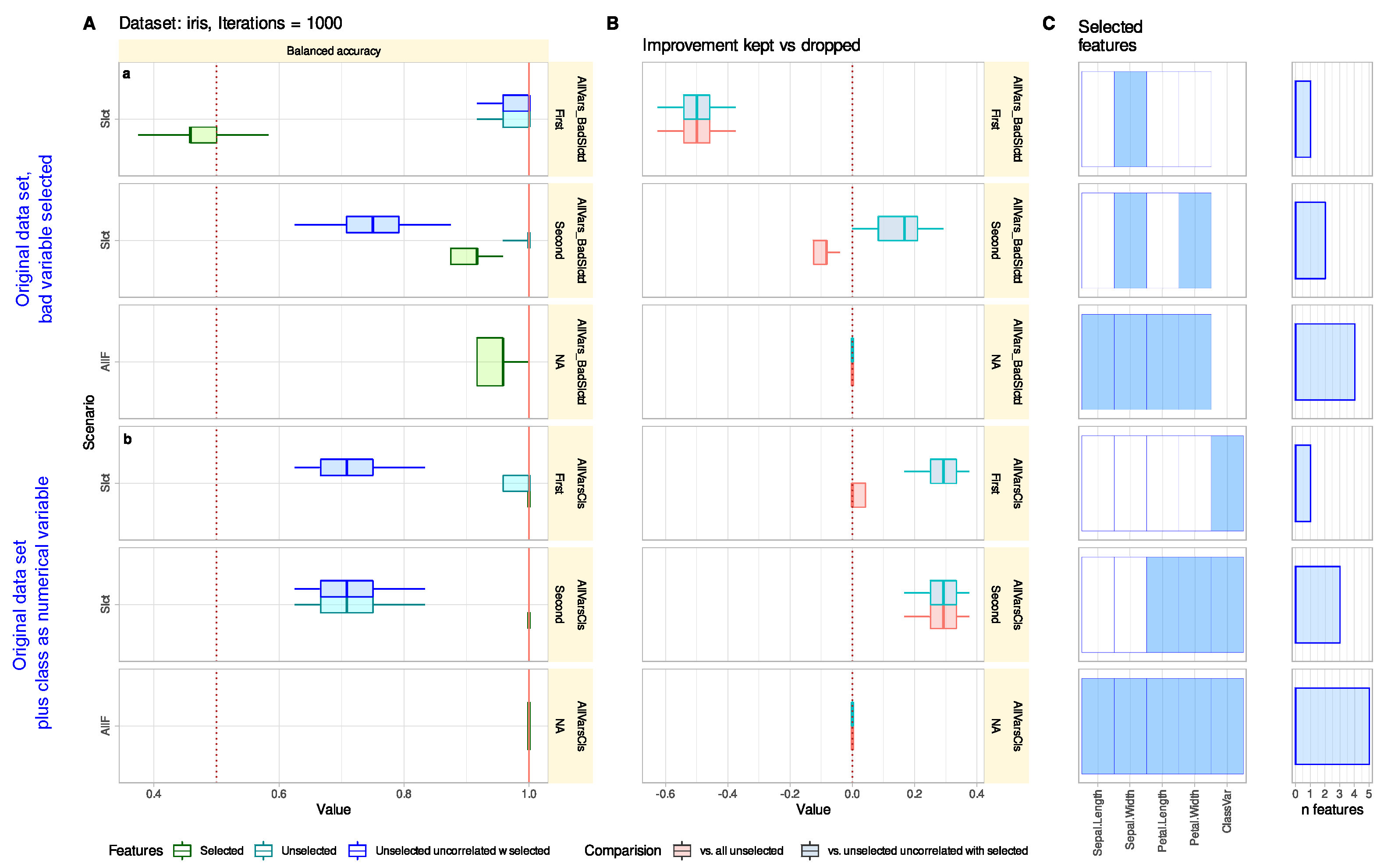
3.1.2. Reconsidering Unselected Features Captures Information When Bad or Trivial Features Were Initially Selected

If the data set contained a variable that is the class membership information, either by mistake or by accidental coincidence, the feature selection will identify that the variable is sufficient to train a perfect classifier (Figure 2) However, there are reasons that renamed class information, or variables identical to class information by any reason, can be a banality in the specific research domain from which the data set originates, and reconsidering the unselected features leads to petal dimension selection as described above, which allows the selected features to be interpreted in the current research field context.

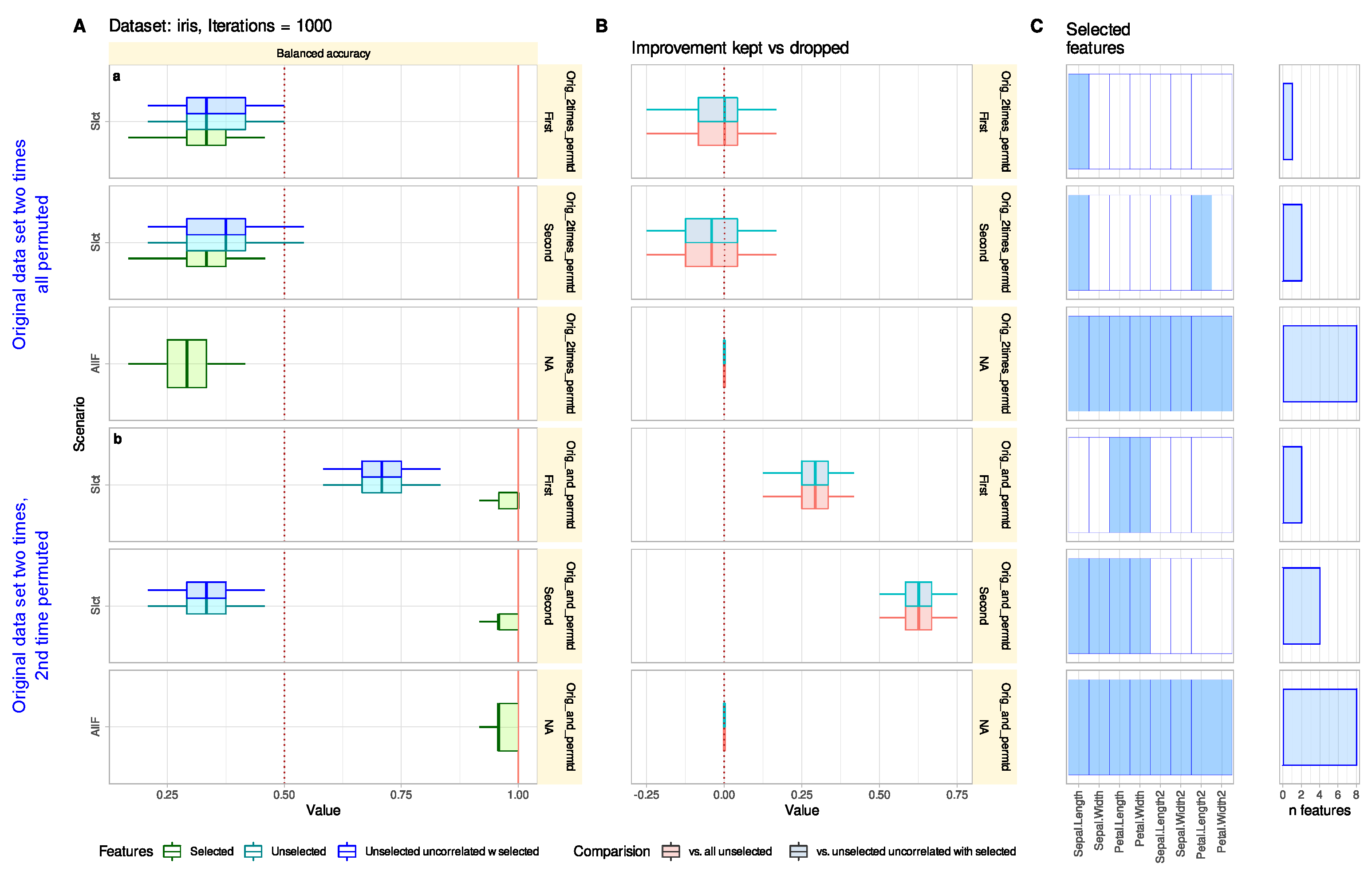
3.1.3. Reconsidering Unselected Features Does Not Tend to Add Uninformative Variables

When permuted versions of the four variables were added to the data set (Figure 3), none of them were selected in either the first or second round of feature selection. In the extreme case, when all variables were permuted (Figure 3 the unsuitability of the then seemingly random selection could be observed immediately from the poor performance of the trained classifiers, with confidence intervals of balanced accuracy 50%. In this case, the difference around zero between the performance of classifiers trained with selected and unselected features clearly indicated that no relevant information had been overlooked in the feature selection.

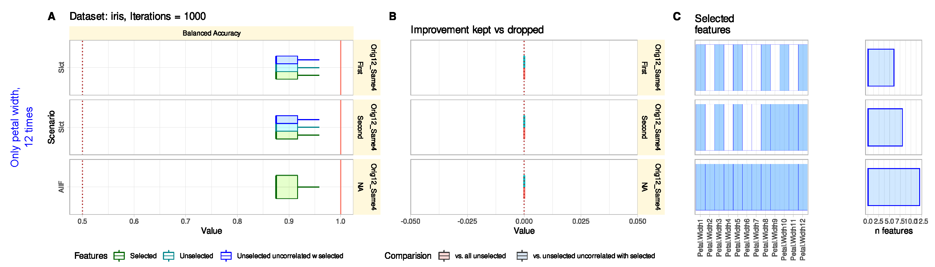
3.1.4. Reconsidering Unselected Features Indicates Relevant Information That May Have Been Missed in The Knowledge Discovery Process

Assembling the data set from similarly informative variables by just repeating the petal width 12 times led to an arbitrary selection of some of the same features (Figure 4), since all features are similarly informative and there is no better feature pick. The classification accuracy was satisfactory because feature selection came at no cost, allowing similar accuracy as when training was conducted with all features. However, training the classifier with the selected features was no better than with the unselected features, and the difference between the balanced accuracies was zero. This clearly indicated an error in feature selection and a need to re-examine the feature set, since it cannot be assumed that the best features were selected from the set of variables. While this may be irrelevant for training classifiers, it is likely relevant for knowledge discovery. Examination of the data set, as indicated by the zero-difference signal, would likely prevent biased interpretation of the selected features that would have gone unnoticed without assessing the classification performance with unselected features.

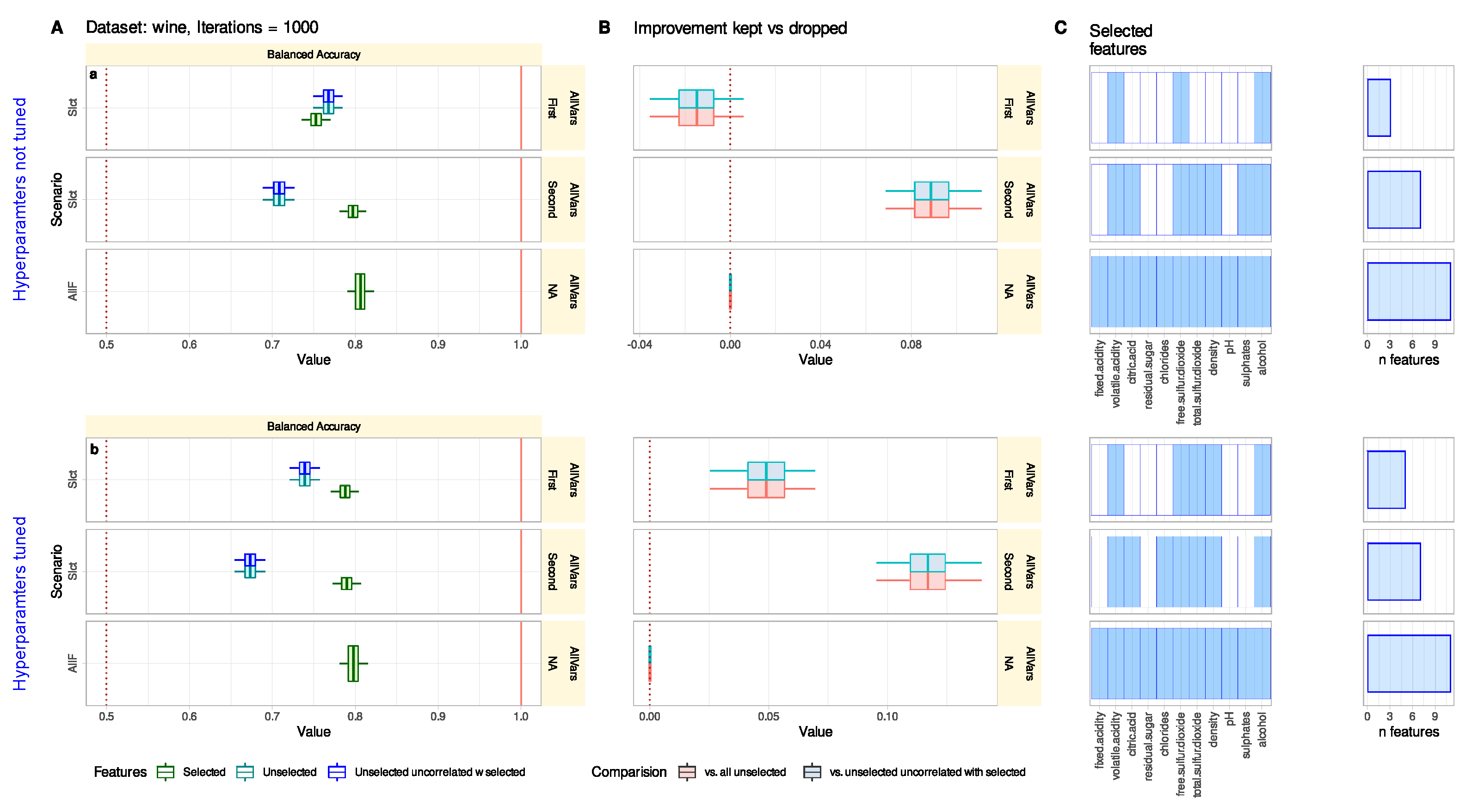
3.2. Wine Quality Data Set

Comparison of Classification Performance with Selected and Unselected Features Can Reveal Feature Selection Problems

When not re-tuning the hyperparameters for the actual data set, feature selection using random forest permutation importance identified alcohol, free sulfur dioxide, and volatile acidity as the best variables for training the algorithm to discriminate between low- and high-quality wines (Figure 5). All of them were included in the result of the fuzzy logic techniques-based identification of relevant predictors of wine quality [31]. Moreover, these are also the variables that were found to be important predictors of wine quality for both wine types in a regression analysis, where red and white wines were evaluated separately [30]. This could have been accepted as a satisfactory result.

However, evaluation of the classification performance obtained when the unselected features were used for training demonstrated that a negative difference (Figure 5A(b)), i.e., it was not better than with the full feature set and, importantly, also not better than with the unselected features. This was indicated by the inclusion of the value zero in the 95% confidence intervals of the differences between the classification performance measures obtained with the selected features versus the full feature set or the non-selected features (Figure 5A(a,b)). The median difference in balanced class assignment accuracy was even smaller than for the unselected characteristics, although it was not significant because the 95% bootstrap confidence interval included the difference of zero.

Following the re-tuning of the random forests for the wine quality data set (see Section 2), the feature selection in the first round already resulted in a larger feature set that was closer to those identified in [30,31] and provided better classification results than the unselected features. This was further improved in the second round when the selected features. The resulting combined feature set thus met both the criterion of achieving classification performance as high as with all features and of selecting those features known from independent evaluations to be relevant to the target.

4. Discussion

This report addresses a typical problem in the analysis of multivariate biomedical data, usually consisting of a set of individuals (cases) belonging to a particular diagnosis (class) and for which multiple measurements have been made (multivariate data). The first question that arises is whether there is any structure in these measurements that is relevant to the class structure and can be used to diagnose (classify) the subjects. To answer this question, a powerful machine-learned classifier can be trained on a subset of the data. If this classifier is able to classify the cases not used in learning (OOB data) such that this classification is close to the true class membership (e.g., a medical diagnosis), this indicates that there is structure in the multivariate data that supports the class structure. This structure could be used to assign future cases to the correct class, e.g., to make an (almost) accurate medical diagnosis for a person about whom the same type of information is available as that on which the algorithm was trained.

However, there are several pitfalls in this context. For example, the diagnosis may be accidentally coded in one or more variables. A typical example is the inclusion of a patient number in the data that contains a numeric code that already indicates the diagnosis. Then, the algorithm is trained on trivial information and is rather useless on future data. Other pitfalls include the problem of correlations and dealing with strongly correlated data. Filtering out correlated variables before machine learning fixes technical sensitivities of algorithms to avoid redundant information. However, this is not necessarily ideal for knowledge discovery. It also requires setting an arbitrary threshold above which the variables are considered highly correlated. A prototypical variable formally selected as the most strongly correlated feature of a group of features may be topically uninformative. On the other hand, selecting a topically meaningful prototype variable may disrupt the data-driven approach to information extraction because it introduces prior assumptions. Intermediate or latent variables computed from the original ones, such as projections onto principal component planes, may be difficult to interpret.

The basic idea presented here is to use the classifier not only for the selected features but also for the unselected features. If the performance of the classifier used is the same for both sets of features, there is no gain in information if only the selected features are used. Moreover, the selected features cannot be claimed to capture the nature of the mechanisms underlying the class structure of the data set. The selected features qualify for valid topical interpretation, if the performance of the classifier is better for the selected features. This is the case if the difference between the performance measures obtained when the algorithm was trained with either the selected features or the unselected features is positive and its 95% confidence interval in cross-validation runs does not include the difference of zero. In such a case, the feature selection can also be considered successful for knowledge discovery or explainable AI. The selected features qualify for valid topical interpretation.

Thus, this report emphasizes that there can be two different goals for feature selection (Figure 6). First, the technical goal of looking for the smallest number of features with which an algorithm can be trained to classify the data with sufficient accuracy (“technical feature selection” (TFS)). Second, the goal of knowledge discovery or XAI, where the features required for successful AI training are also interpreted in the topical context of the research data. In this scenario, the set of features must allow the, e.g., medical, field expert to understand how a machine system for class assignment, e.g., diagnosis, proceeds in order to arrive at a sufficiently accurate diagnosis. (“explainable feature selection” (XFS)). This might require more features than are technically necessary for a successful classification to enable a logical chain of reasoning that explains the class assignment within the particular research area. Thus, there can be different solutions for feature selection depending on the topical context and final aim of the analysis. The proposed approach facilitates explainable AI [2] because experts in the field will better understand an AI’s decision if the key features on which the decision is based make sense to them in the context of their expertise, rather than simply accepting that the “black box” algorithm can use the information to make a diagnosis, to remain in the medical example.

Moreover, as demonstrated with the wine quality data set, the proposed method implicitly provides a signal for pathologies in feature selection that might escape attention without the reexamination of the unselected features. In machine learning reports, usually only the performance of the classifiers trained with the selected features is compared to the performance obtained when all variables were used for training. Given that feature selection methods can produce biased results [14,15], the proposed method provides a signal to identify missing informative variables and ensure that the most appropriate features were indeed selected for classifier training. To ensure that the best features were selected, the classifier performance when the unselected features were used for training should also be reported. There are valid reasons why performances may not be different, e.g., strongly correlated variables across selected and unselected features. However, this can be easily identified and interpreted to provide a complete picture of the information contained in the selected features compared to all variables. Moreover, the present example with the wine quality data set reemphasizes that random forests benefit from hyperparameter tuning, despite the suggestions to the contrary cited above and consistent with a recent case, published separately [23].

Limitations of the present assessments include the limited choice of machine-learning methods. While the proposed method should be generally suitable for the machine learning-based feature selection, here it was tested only with the OOB permutation feature importance of random forests. In addition, only one measure of classification performance was used, namely balanced accuracy. In the present experiments, the area under the receiver operating characteristic [34] was calculated in parallel, but it did not provide any additional insight, but merely repeated the observations based on the balanced accuracy, and therefore, for brevity, it is not included in the report. It is advisable to test the utility of further classification performance measures in the present XFS context separately when needed.

It should be noted that the present evaluations did not aim at benchmarking feature selection procedures for classification problems, but mainly at the importance of re-testing unselected features before declaring a machine learning-based analysis of a data set complete. In a review of feature selection methods for bioinformatics, especially for disease risk prediction [4], a classification was proposed according to which the approach proposed in the present report, especially to consider the unselected features, would belong to the class of feature selection algorithms that are independent of the details of the particular classifier algorithm. The other methods, on the other hand, depend on the details of the classifier algorithm. In particular, the approach presented here does not depend on the details of a particular feature selection algorithm or on a particular method for computing feature importance. In [35], different methods for evaluating the performance of different algorithms are compared with the result that none of them has a clear advantage. Moreover, the present experiments were conducted with classification problems. The re-evaluation of unselected features in regression problems has not been explicitly addressed. This would require the specification of modified signals, since balanced accuracy addresses classification, while an analogous measure must be found for regression before extending the currently proposed method to regression problems.

5. Conclusions

This work is particularly concerned with the features that are discarded by feature selection algorithms. When a classification task is attempted with such features omitted, there are two possible outcomes: The task fails or the task is possible even with the features not considered. If the task fails with the features not considered, then the conclusion is valid that the feature selection has chosen the best features for the task. If the classification is still possible, then either other features can be selected or the feature selection algorithm is not working correctly. If the algorithm is working correctly, then feature set can be extended to features that well describe the data generation process from an expert’s point of view. Thus, the present proposal makes a distinction between whether the feature set can be described as containing relevant information for class assignment or whether as containing the only relevant information for class assignment. The former allows the unselected features to be included in the mechanistic interpretation, while the latter excludes them, i.e., adds a logical “NOT” to the argument in the sense of “these features are relevant, but not those”. Thus, we propose, in line with [4], that extracting a subset of the most relevant features (through feature selection) could help researchers to understand the biological process(es) that underlie the disease.

Reconsideration of originally unselected items in multivariate data sets is proposed as a method to enhance the topical interpretation of variables emerging from feature selection aimed at knowledge discovery or explainable machine learning. This can be useful to filter out uninformative or trivial information or to add relevant topical information from variables originally overlooked in the feature selection. In addition, it can help to detect pathologies and errors in the feature selection that occasionally fail to identify the most appropriate variables. The method is generic to feature selection methods based on the supervised machine learning-based and can be implemented in the feature selection workflows.

References

1. Guyon, I. An introduction to variable and feature selection. J. Mach. Learn. Res. 2003, 3, 1157–1182. [Google Scholar]
2. Lotsch, J.; Kringel, D.; Ultsch, A. Explainable Artificial Intelligence (XAI) in Biomedicine: Making AI Decisions Trustworthy for Physicians and Patients. BioMedInformatics 2022, 2, 1. [Google Scholar] [CrossRef]
3. Miller, G.A. The magical number seven plus or minus two: Some limits on our capacity for processing information. Psychol. Rev. 1956, 63, 81–97. [Google Scholar] [CrossRef] [PubMed] [Green Version]
4. Pudjihartono, N.; Fadason, T.; Kempa-Liehr, A.W.; O’Sullivan, J.M. A Review of Feature Selection Methods for Machine Learning-Based Disease Risk Prediction. Front. Bioinform. 2022, 2, 927312. [Google Scholar] [CrossRef]
5. Saeys, Y.; Inza, I.; Larranaga, P. A review of feature selection techniques in bioinformatics. Bioinformatics 2007, 23, 2507–2517. [Google Scholar] [CrossRef] [Green Version]
6. Yu, L.; Liu, H. Feature Selection for High-Dimensional Data: A Fast Correlation-Based Filter Solution. In Proceedings of the Twentieth International Conference on Machine Learning (ICML-2003), Washington, DC, USA, 21–24 August 2003. [Google Scholar]
7. Aboudi, N.E.; Benhlima, L. Review on wrapper feature selection approaches. In Proceedings of the 2016 International Conference on Engineering & MIS (ICEMIS), Agadir, Morocco, 22–24 September 2016; pp. 1–5. [Google Scholar]
8. Chen, C.W.; Tsai, Y.H.; Chang, F.R.; Lin, W.C. Ensemble feature selection in medical datasets: Combining filter, wrapper, and embedded feature selection results. Expert Syst. 2020, 37, e12553. [Google Scholar] [CrossRef]
9. Santosa, F.; Symes, W.W. Linear Inversion of Band-Limited Reflection Seismograms. Siam J. Sci. Stat. Comput. 1986, 7, 1307–1330. [Google Scholar] [CrossRef]
10. Ho, T.K. Random Decision Forests. In Proceedings of the 3rd International Conference on Document Analysis and Recognition, Montreal, QC, Canada, 14–16 August 1995. [Google Scholar] [CrossRef]
11. Breiman, L. Random Forests. Mach. Learn. 2001, 45, 5–32. [Google Scholar] [CrossRef] [Green Version]
12. Kursa, M.B.; Rudnicki, W.R. Feature Selection with the Boruta Package. J. Stat. Softw. 2010, 36, 1–13. [Google Scholar] [CrossRef] [Green Version]
13. Liaw, A.; Wiener, M. Classification and Regression by randomForest. R N. 2002, 2, 18–22. [Google Scholar]
14. Parr, T.; Turgutlu, K.; Csiszar, C.; Howard, J. Beware Default Random Forest Importances 2018. Available online: https://explained.ai/rf-importance (accessed on 3 September 2022).
15. Strobl, C.; Boulesteix, A.L.; Zeileis, A.; Hothorn, T. Bias in random forest variable importance measures: Illustrations, sources and a solution. BMC Bioinform. 2007, 8, 25. [Google Scholar] [CrossRef]
16. Ultsch, A.; Lotsch, J. Computed ABC Analysis for Rational Selection of Most Informative Variables in Multivariate Data. PLoS ONE 2015, 10, e0129767. [Google Scholar] [CrossRef] [Green Version]
17. Juran, J.M. The non-Pareto principle; Mea culpa. Qual. Prog. 1975, 8, 8–9. [Google Scholar]
18. Lotsch, J.; Ultsch, A. Random Forests Followed by Computed ABC Analysis as a Feature Selection Method for Machine Learning in Biomedical Data; Advanced Studies in Classification and Data Science; Springer: Singapore, 2020; pp. 57–69. [Google Scholar]
19. Ihaka, R.; Gentleman, R. R: A Language for Data Analysis and Graphics. J. Comput. Graph. Stat. 1996, 5, 299–314. [Google Scholar] [CrossRef]
20. R Core Team. R: A Language and Environment for Statistical Computing. Available online: https://www.R-project.org/ (accessed on 3 September 2022).
21. Kuhn, M. Caret: Classification and Regression Training. 2018. Available online: https://cran.r-project.org/package=caret (accessed on 3 September 2022).
22. Lötsch, J.; Malkusch, S.; Ultsch, A. Optimal distribution-preserving downsampling of large biomedical data sets (opdisDownsampling). PLoS ONE 2021, 16, e0255838. [Google Scholar] [CrossRef]
23. Lötsch, J.; Mayer, B. A Biomedical Case Study Showing That Tuning Random Forests Can Fundamentally Change the Interpretation of Supervised Data Structure Exploration Aimed at Knowledge Discovery. BioMedInformatics 2022, 2, 544–552. [Google Scholar] [CrossRef]
24. Good, P.I. Resampling Methods: A Practical Guide to Data Analysis; Birkhauser: Boston, MA, USA, 2006. [Google Scholar]
25. Tille, Y.; Matei, A. Sampling: Survey Sampling. 2016. Available online: https://cran.r-project.org/package=sampling (accessed on 3 September 2022).
26. Brodersen, K.H.; Ong, C.S.; Stephan, K.E.; Buhmann, J.M. The Balanced Accuracy and Its Posterior Distribution. In Proceedings of the 2010 20th International Conference on Pattern Recognition (ICPR), Istanbul, Turkey, 23–26 August 2010; pp. 3121–3124. [Google Scholar] [CrossRef]
27. Anderson, E. The irises of the Gaspe peninsula. Bull. Am. Iris Soc. 1935, 59, 2–5. [Google Scholar]
28. Fisher, R.A. The use of multiple measurements in taxonomic problems. Ann. Eugen. 1936, 7, 179–188. [Google Scholar] [CrossRef]
29. Bannerman-Thompson, H.; Bhaskara Rao, M.; Kasala, S. Chapter 5-Bagging, Boosting, and Random Forests Using R. In Handbook of Statistics; Rao, C.R., Govindaraju, V., Eds.; Elsevier: Amsterdam, The Netherlands, 2013; Volume 31, pp. 101–149. [Google Scholar] [CrossRef]
30. Gupta, Y.K. Selection of important features and predicting wine quality using machine learning techniques. Procedia Comput. Sci. 2018, 125, 305–312. [Google Scholar] [CrossRef]
31. Nebot, A.; Mugica, F.; Escobet, A. Modeling Wine Preferences from Physicochemical Properties using Fuzzy Techniques. In Proceedings of the 5th International Conference on Simulation and Modeling Methodologies, Technologies and Applications—SIMULTECH, Colmar, France, 21–23 July 2015. [Google Scholar] [CrossRef] [Green Version]
32. Schober, P.; Boer, C.; Schwarte, L.A. Correlation Coefficients: Appropriate Use and Interpretation. Anesth. Analg. 2018, 126, 1763–1768. [Google Scholar] [CrossRef]
33. Spearman, C. The proof and measurement of association between two things. Am. J. Psychol. 1904, 15, 72–101. [Google Scholar] [CrossRef]
34. Peterson, W.; Birdsall, T.; Fox, W. The theory of signal detectability. Trans. Ire Prof. Group Inf. Theory. 1954, 4, 171–212. [Google Scholar] [CrossRef]
35. Khaire, U.M.; Dhanalakshmi, R. Stability of feature selection algorithm: A review. J. King Saud Univ.-Comput. Inf. Sci. 2022, 34, 1060–1073. [Google Scholar] [CrossRef]
Figure 1. Feature selection and classification performance evaluation with different feature sets in the iris data set [28]. The graph is divided into subgraphs a–c from top to bottom. Experiments were performed (a) with the original data, (b) with the iris data set omitting one highly correlated variable, and (c) with the data set adding all variables twice. Each subgraph is organized in three further subgraphs, showing from top to bottom (i) the results when using the features selected in the default feature selection, (ii) the features added when performing a second feature selection on the unselected features from the first selection, and (iii) when training the algorithm with the full feature set. The boxes show the 25th, 50th (blue vertical line), and 75th percentiles of balanced accuracies obtained in 1000 repeated runs with a random selection of 67% from the training data set and 80% from a validation data set separated from the data set before feature selection. Whiskers span the 95% confidence interval from the 2.5th to the 97.5th percentiles. (A): Balanced accuracy obtained with a random forests classifier trained with (i) the selected features, (ii) the unselected features, and (iii) the unselected features that were not highly correlated with the selected features, with the correlation threshold set at a very strong correlation of ρ > 0.9. (B): Difference in balanced accuracy when algorithms were trained with the selected versus unselected features. (C): Selected features (blue) and unselected features (white). Features excluded from the experiments due to very strong correlation are shown in gray.
Biomedinformatics 02 00047 g001
Figure 2. Feature selection and classification performance evaluation with different feature sets in the iris data set [28]. The graph is divided into subgraphs a–b from top to bottom. Experiments were performed (a) with the original data but sepal length was defined to be selected in a first run of feature selection, (b) with the iris data set where the class information was added as a numerical variable. Each subgraph is organized in three further subgraphs, showing from top to bottom (i) the results when using the features selected in the default feature selection, (ii) the features added when performing a second feature selection on the unselected features from the first selection, and (iii) when training the algorithm with the full feature set. The boxes show the 25th, 50th (blue vertical line), and 75th percentiles of balanced accuracies obtained in 1000 repeated runs with a random selection of 67% from the training data set and 80% from a validation data set separated from the data set before feature selection. Whiskers span the 95% confidence interval from the 2.5th to the 97.5th percentiles. (A): Balanced accuracy obtained with a random forests classifier trained with (i) the selected features, (ii) the unselected features, and (iii) the unselected features that were not highly correlated with the selected features, with the correlation threshold set at a very strong correlation of ρ > 0.9. (B): Difference in balanced accuracy when algorithms were trained with the selected versus unselected features. (C): Selected features (blue) and unselected features (white).
Biomedinformatics 02 00047 g002
Figure 3. Feature selection and classification performance evaluation with different feature sets in the iris data set [28]. The graph is divided into subgraphs a - b from top to bottom. Experiments were performed (a) with doubling each variable and randomly permuting all variables, (b) doubling the data set and randomly permuting the second version of each variable while leaving the first versions in their original stage. Each subgraph is organized in three further subgraphs, showing from top to bottom (i) the results when using the features selected in the default feature selection, (ii) the features added when performing a second feature selection on the unselected features from the first selection, and (iii) when training the algorithm with the full feature set. The boxes show the 25th, 50th (blue vertical line), and 75th percentiles of balanced accuracies obtained in 1000 repeated runs with a random selection of 67% from the training data set and 80% from a validation data set separated from the data set before feature selection. Whiskers span the 95% confidence interval from the 2.5th to the 97.5th percentiles. (A): Balanced accuracy obtained with a random forests classifier trained with (i) the selected features, (ii) the unselected features, and (iii) the unselected features that were not highly correlated with the selected features, with the correlation threshold set at a very strong correlation of ρ > 0.9. (B): Difference in balanced accuracy when algorithms were trained with the selected versus unselected features. (C): Selected features (blue) and unselected features (white).
Biomedinformatics 02 00047 g003
Figure 4. Feature selection and classification performance evaluation with different feature sets in the iris data set [28]. Experiments were performed only on petal width, added 12 times to the data set. The graph is organized in three subgraphs, showing from top to bottom (i) the results when using the features selected in the default feature selection, (ii) the features added when performing a second feature selection on the unselected features from the first selection, and (iii) when training the algorithm with the full feature set. The boxes show the 25th, 50th (blue vertical line), and 75th percentiles of balanced accuracies obtained in 1000 repeated runs with a random selection of 67% from the training data set and 80% from a validation data set separated from the data set before feature selection. Whiskers span the 95% confidence interval from the 2.5th to the 97.5th percentiles. (A): Balanced accuracy obtained with a random forests classifier trained with (i) the selected features, (ii) the unselected features, and (iii) the unselected features that were not highly correlated with the selected features, with the correlation threshold set at a very strong correlation of ρ > 0.9. (B): Difference in balanced accuracy when algorithms were trained with the selected versus unselected features. (C): Selected features (blue) and unselected features (white).
Biomedinformatics 02 00047 g004
Figure 5. Feature selection and classification performance evaluation with different feature sets in the wine quality data set from https://www.kaggle.com/datasets/shelvigarg/wine-quality-dataset (accessed 2 November 2022). The graph is divided into subgraphs a–b from top to bottom. Experiments were performed (a) with non-tuned (a) and tuned (b) hyperparameters. The two subgraphs show from top to bottom (i) the results when using the features selected in the default feature selection, (ii) the features added when performing a second feature selection on the unselected features from the first selection, and (iii) when training the algorithm with the full feature set. The boxes show the 25th, 50th (blue vertical line), and 75th percentiles of balanced accuracies obtained in 1,000 repeated runs with a random selection of 67% from the training data set and 80% from a validation data set separated from the data set before feature selection. Whiskers span the 95% confidence interval from the 2.5th to the 97.5th percentiles. (A): Balanced accuracy obtained with a random forests classifier trained with (i) the selected features, (ii) the unselected features, and (iii) the unselected features that were not highly correlated with the selected features, with the correlation threshold set at a very strong correlation of ρ > 0.9. (B): Difference in balanced accuracy when algorithms were trained with the selected versus unselected features. (C): Selected features (blue) and unselected features (white).
Biomedinformatics 02 00047 g005
Figure 6. Flowchart showing the proposed feature selection workflow, with a distinction of the final goal into (i) “technical feature selection” (TFS), where the goal can be defined as training a powerful classifier, and (ii) “explainable feature selection” (XFS), where the goal can be defined that the selected features should be interpretable by a domain expert. Based on the evaluation of whether the entire input data space has a structure that matches the class structure of the output data space, for TFS the selected features are sufficient if the classifier computes the classification with the same accuracy as with all features in the data set. However, relevant information that makes the feature sets interpretable by the expert in the field may be lost in the process. For XFS, the selected features should therefore be interpretable by an expert in the field, i.e., they should contain relevant variables that provide information about the processes underlying the class structure. This can be facilitated by including the initially unselected features in the interpretation, as proposed in this report, or alternatively by reducing the data set to a bare informative minimum.
Biomedinformatics 02 00047 g006
Publisher’s Note: MDPI stays neutral with regard to jurisdictional claims in published maps and institutional affiliations.