Article

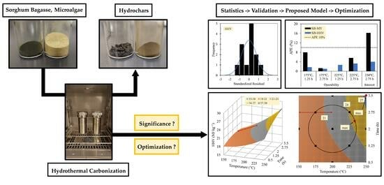
Significance and Optimization of Operating Parameters in Hydrothermal Carbonization Using RSM–CCD

Graduate School of Bioresources, Mie University, Tsu 514-8507, Japan
*
Author to whom correspondence should be addressed.
Thermo 2024, 4(1), 82-99; https://doi.org/10.3390/thermo4010007
Submission received: 16 January 2024 / Revised: 12 February 2024 / Accepted: 14 February 2024 / Published: 18 February 2024
(This article belongs to the Special Issue Lifetime Prediction of Polymeric Materials)

Abstract

:
To ascertain the significance of temperature and residence time of hydrothermal carbonization (HTC) in controlling hydrochar production, multiple regression was employed based on central composite design (CCD) to model the responses of mass yield (MY) and higher heating value (HHV). The hydrothermal reaction was explored at temperatures and times ranging from 150 to 250 °C and 0.5 to 3.5 h. Sorghum bagasse (SB) and microalgae (MA) were used to complex the reaction due to their differences in organic constituents. Simultaneously, the operating parameters were optimized by maximizing the response values under domain constraints in the HHV models. The results show that at least temperature and time in the linear system played a significant role in determining the solids recovery and the energy generation of hydrochars (p-values = 0.00), regardless of the biomass type. Moreover, the optimum conditions of SB and MA hydrochars can be achieved by increasing the temperature to the limit of 250 °C and prolonging the time to 3.5 and 3.25 h, respectively. Both respective conditions resulted in maximum HHVs of 27.54 and 35.83 MJ kg−1.

Graphical Abstract

1. Introduction

Hydrothermal carbonization (HTC) is an artificial coalification process that converts organic compounds into carbonaceous materials in hot pressurized water. The process is largely governed by important operating parameters such as temperature and residence time [1]. The reaction occurs in subcritical water at a relatively low temperature of 150–250 °C, accompanied by an autogenous pressure elevation of about 2–6 MPa [2,3]. Various residence times are practically used, ranging from 5 to 240 min [4], although the reaction seems evident within the first 30 min [5]. Temperature plays a role in reducing the dielectric properties of water. Owing to the diminishing of hydrogen bonds and the formation of ionization products, such as hydronium (H3O+) and hydroxide ions (OH), the dissociation constant expands by three orders of magnitude as the critical point approaches, which makes temperature a determinant of acid- and base-catalyzed reactions [6]. Meanwhile, the retention time enhances the severity of the reaction at a given temperature [7].
In some cases, the effects of operating parameters cannot be observed for some biomasses due to insignificant responses. For example, using residual corn cob and biogas digestate, Zhang et al. [5] and Cao et al. [8] reported that the residence times of 0.5–5 h (at 250 °C) and 0.5–6 h (at 210 °C) did not cause significant changes in the heating values of the hydrochars produced. The deviation values were shown to be less than 1.5 and 0.3 MJ kg−1, respectively. Such circumstances may render further experimental studies intensive and time-consuming [9]. Therefore, pre-identifying the significance of the operating parameters becomes essential, and an appropriate experimental design will be required for assessment.
To further investigate the operating parameters, extensive studies on fuel properties such as mass yield (MY) and higher heating value (HHV) may well describe the conversion process. Particularly for optimization, HHV is the most important response that displays the maximum amount of energy generation and determines the conversion efficiency [10,11]. For example, Prins et al. [12] found that biomasses with different heating values were recommended to approach the highest gasification efficiency under different temperatures. Moreover, HHV has direct implications for chemical structures as it can be approximated by proximate and ultimate characteristics [13,14]. An adiabatic calorimeter analysis is often performed to determine HHV. However, the analysis is considered time-consuming and expensive for a large number of runs [10]. Thereby, building an empirical model is a key tool in analyzing and optimizing the conversion process while avoiding time-consuming experiments.
The response surface method (RSM) is an experimental design that simultaneously allows the significance estimation and the optimization between factors and responses. The model fitting involves not only the main and interaction effects but also the quadratic effects. Accordingly, RSM design can provide an idea of the local shape of the response surface [15,16]. A k-factor three-level factorial design (3k FD) is least required for detecting pure quadratic effects in RSM, although not for their estimation. On the other hand, the 3k FD suffers from the major drawbacks of a large number of experimental runs and a lack of rotatability (a non-uniformity of prediction errors). Prior to a study, little or no knowledge may be present regarding the domain that contains the optimum response. Therefore, such an experimental design matrix may obscure the investigation in any direction. A modified design, such as central composite design (CCD), exists to overcome these concerns. CCD features a variance of the predicted response, which is a function of the distance from the center point instead of a function of the direction [15,17].
Based on this overview, this study explores the operating parameters of temperature and residence time using RSM–CCD as a multivariate statistical method. Multiple regression and analysis of variance (ANOVA) are performed for the model approach and diagnostic tests. Sorghum bagasse (SB) and microalgae (MA) are used to complex the biomass types by representing lignocellulosic (LBM) and non-lignocellulosic biomass (NLBM). The objectives of this study are (1) to estimate the significance of temperature and time in controlling MY and HHV properties, and (2) to predict the optimum conditions that result in maximum output from the empirical HHV models.

2. Materials and Methods

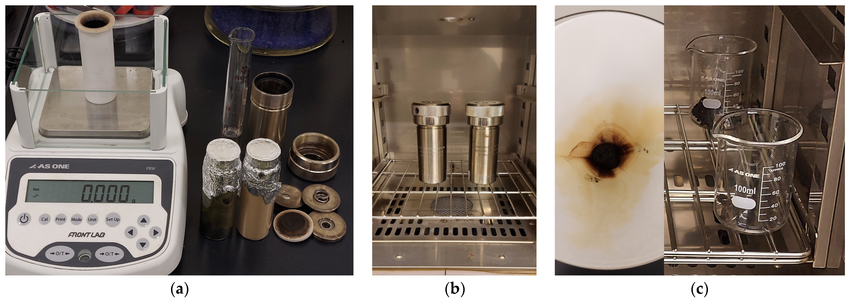
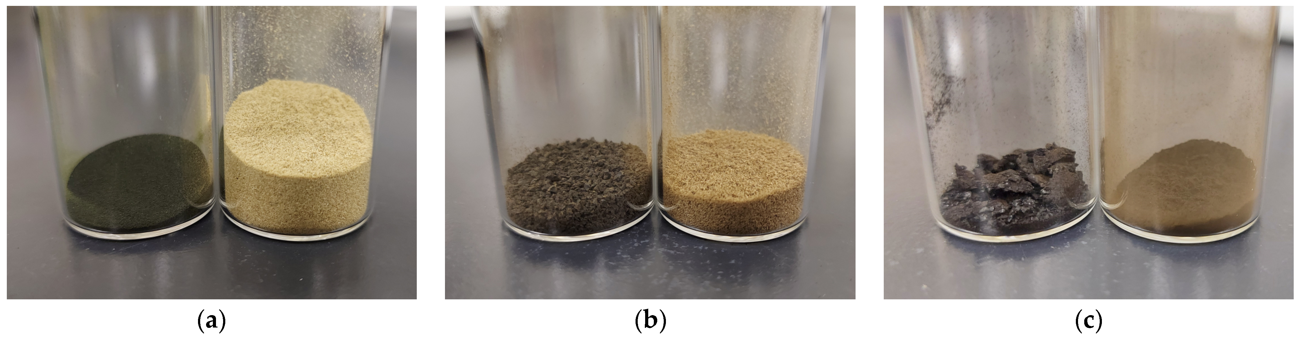
2.1. Sample Preparation

All plant parts of SB were collected from the experimental farm of Mie University, Japan, except the roots. SB was washed, air-dried, mechanically pulverized using a high-speed blender (YKB, AS ONE Corp., Osaka, Japan) at 28,000 rpm for 1 min, and sieved until a uniform powder size of less than 150 μm was obtained. Meanwhile, MA (Chlorella sp.) was purchased in powder form under the trademark of Sunlife Co. Ltd. All raw biomasses were dried in a laboratory oven at 105 °C for 24 h to homogenize the moisture content. The homogenized samples were then stored in a desiccator prior to further experiments. The biochemical composition of the similar biomasses is reviewed in Table 1.

2.2. Hydrothermal Carbonization Experiment

In each batch of HTC experiments, a mixture of 3.5 g dried biomass and 35 g deionized water was synthesized in a 45 mL digestion vessel (Model 4744, Parr Instrument Co., Moline, IL, USA), followed by oven-assisted heating (OF-300V, AS ONE Corp., Osaka, Japan) (see Figure 1a,b). The heating treatment applied temperatures and residence times ranging from 150 °C to 250 °C and 0.5 to 3.5 h, with CCD factor levels described later in Section 2.4. After completion, the vessel was aerated using a fan to speed the cooling to 27 °C. The slurry obtained was subjected to gravity filtration to separate the residual solids from the aqueous phase (see Figure 1c). Finally, the solids were dried at 105 °C for 24 h to recover the final products, referred to as hydrochars (see Figure 2).

2.3. Data Analysis

Two responses of MY and HHV were evaluated as the representative fuel properties of hydrochars produced. MY (in %) shows the amount of solids that can be recovered after HTC. The response was calculated from the ratio between the mass of hydrochar produced, mH (in kg), and dried biomass, mB (in kg), which is expressed as follows:
M Y = m H m B × 100 % ,
Meanwhile, HHV (in MJ kg−1) was sought using an adiabatic calorimeter (OSK 150, Ogawa Sampling Co., Ltd., Tokyo, Japan) to measure heat release, which includes the latent heat of the evaporation. A sample weighing 0.3 g was subjected to complete combustion for each experiment. The bomb was installed under a pressurized oxidative environment by injecting O2 until it reached 3 MPa. HHV was calculated based on Equation (2), which also involves its correction factors:
H H V = c W Δ T M + m W m P C P Δ m R C R 10 6 × m S ,
where mS, mW, and mP are the masses of sample, water, and wrapping paper (in kg). The mass of water in the bucket is fixed at 1.5 kg. ∆mR is the mass loss of ignition wire after combustion (in kg). M is the equivalent mass of water, standardized at 0.3222 kg by combusting benzoic acid. cW is the specific heat capacity of water, which is 4200 J kg−1 °C−1. CP and CR are the heat capacities of paper and wire (J kg−1). The heat capacities are 15,070 × 103 and 3035 × 103 J kg−1, respectively. ∆T is the temperature rise of water after combustion (in °C).

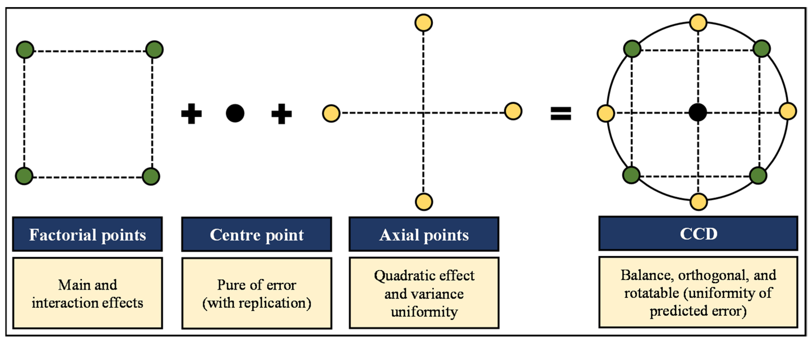
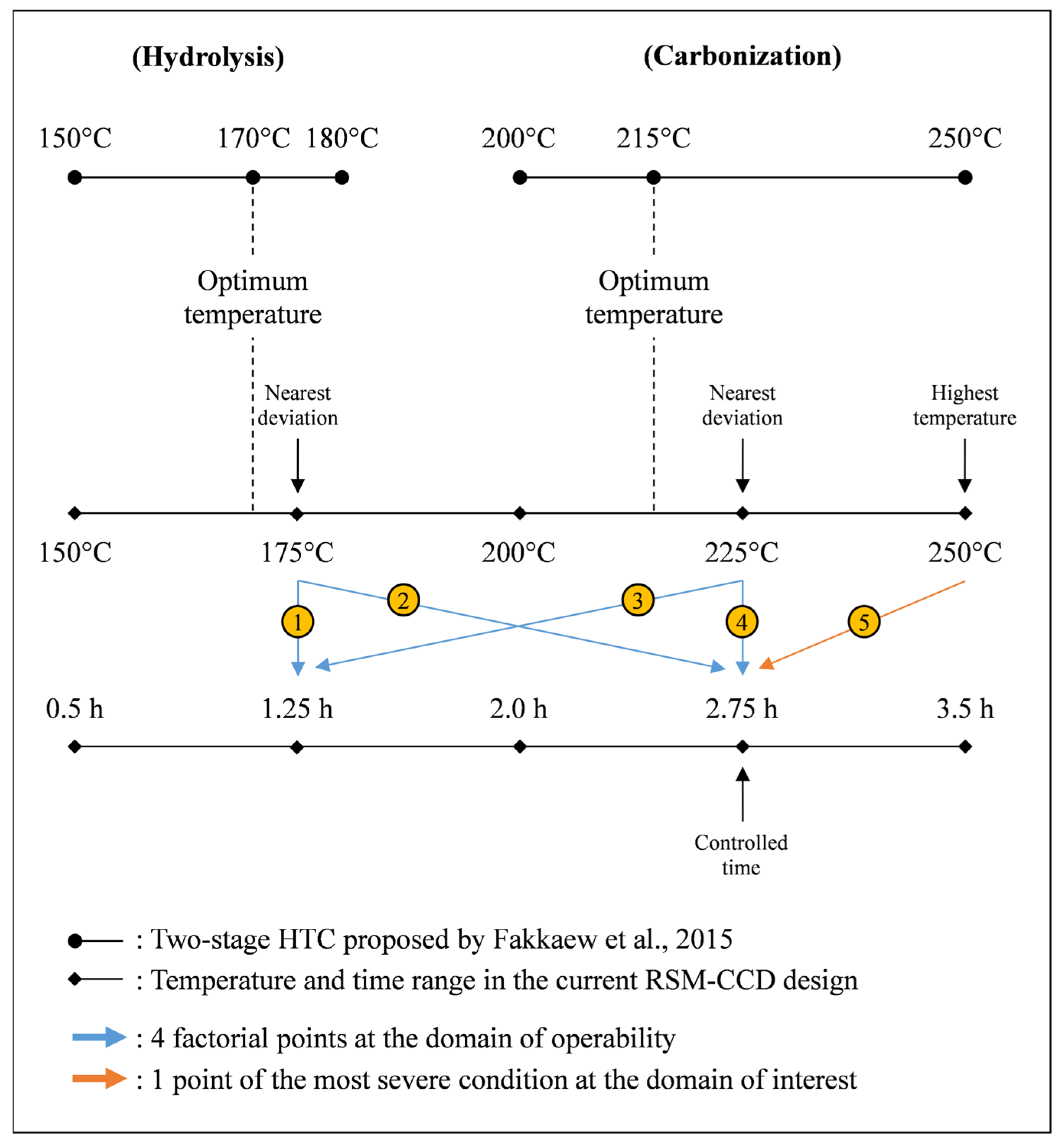
2.4. Experimental Design and Diagnostic Test

RSM was adopted to evaluate the curvature effect on the correlation between operating parameters and fuel properties. The CCD was implemented by having a fractional factorial with two levels (±1) from the center point (0), which was augmented with a group of axial points spaced |α| ≥ 1.414 (domain of operability). The space design was chosen to meet the desired properties of being balanced, orthogonal, and rotatable [15]. Temperature and time were evaluated as operating parameters or factors, ranging from 150 °C to 250 °C and 0.5 to 3.5 h (domain of interest). The experimental design with five coded factor levels and their actual values is shown in Table 2. The full run consisted of five center points, four factorial points, and four axial points (α = ±2) (see Table 3 and Appendix A Figure A1). The axial points were customized by 2, instead of the original value of 1.414, to maximize the viability limit of uniformity of the predicted errors [17].
The general linear model (GLM) was applied as a statistical option using IBM SPSS 28.0 software. The full quadratic regression function was then estimated as expressed by Equation (3) [16,23]:
y = β 0 + i = 1 k β i x i + i = 1 k β i i x i   2 + 1 i j k β i j x i x j + ε ,
where k is the number of factors. β0 is the intercept coefficient. βi, βii, and βij are the coefficients of linear, quadratic, and interaction systems, respectively. y and xi,j are the pertinent responses and factors, respectively. ε is the mean error or residual term (assumed to be zero if normally distributed). Meanwhile, diagnostic tests were premised on the fulfillment of several principles proposed by Sarstedt and Mooi [24], namely (1) model fit (goodness of fit), (2) assumption of regression model least in a linear coefficient, (3) residual assumptions of regression model, and (4) multicollinearity among factors. ANOVA was used to assess the overall model and its factor systems, considering a confidence level of 95%. The coefficient of determination (R2), the probability value (p-value) of Fischer distribution (F-test), and the residual plots were subsequently evaluated.

2.5. Data Validation

The models were validated by assigning new datasets to see the accuracy of the predicted data (see Appendix A Figure A2). Four new observational data were drawn from factorial points within the domain of operability. One datum was taken from an additional point at x1 = 2 (250 °C) and x2 = 1 (2.75 h), beyond the domain of operability but still occupying the domain of interest. The relative error between the observed (yo) and predicted responses (yp) was scored by the absolute percentage error, APE (in %). The scoring possesses an intuitive interpretability and is scale-independent. To avoid measurement bias, the response should be strictly positive and have no zero or near-zero values [25,26]. APE is expressed as the following equation:
A P E = y o y p y o × 100 % ,

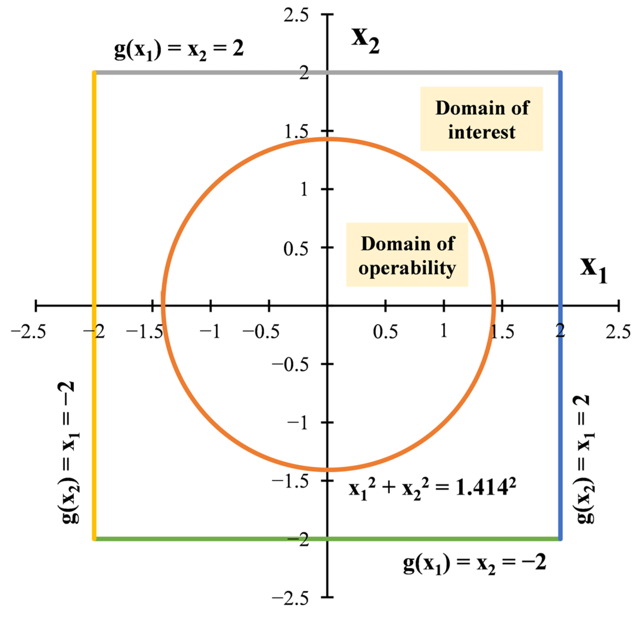
2.6. Optimum Conditions

The optimum condition of HTC was determined by maximizing the HHV response, which was indicated by the critical point. The coordinate was determined through the first derivative of the regression function being equal to zero (see Equation (5)). Such a critical point is likely to be found in a model with maximum, minimum, or saddle profiles [16]. Supposing the coordinate of the critical point lies outside the domain of interest, the maximum point can be found by the constraint optimization. The regression function is thus moved in the −∇y or +∇y direction as infinite steps of x1 and x2 until the contour hits the domain boundary [27,28]. In this study, there were two methods used: (1) single variable (for domain of interest) and (2) Lagrange multiplier (for domain of operability).
y x 1 = 0 ,   y x 2 = 0 ,
For the domain of interest, the constant functions of the square-shaped boundary and the highest and lowest domain ranges were simply substituted into the regression function as coordinate pairs (see Equations (6) and (7) and Figure 3). The highest response among all the boundary sides was determined as the maximum point. Occasionally, if the substitution of the constant function generates a quadratic form, the other coordinate pair is sought from its first derivative, which is equal to zero, as seen in Equation (8).
g x 1 = x 2 = c ,   g x 2 = x 1 = c ,
D i = x 1 , x 2 | 2 x 1 2 , 2 x 2 2 ,
y x 1 , c x 1 = 0 ,   y c , x 2 x 2 = 0 ,
On the other hand, for the domain of operability, the Lagrange multiplier solved the boundary function (g) that has the same input variables as the regression function (y(x1,x2)) and can be expressed as g(x1,x2) = c. The equation is proposed from the tangency between the regression function and the boundary function, whose gradients are parallel to each other, as follows [28]:
y x 1 , x 2 = λ g x 1 , x 2 ,
where λ is the proportionality constant, called the Lagrangian. The boundary function in circular shape is defined in Equation (10) (see Figure 3). To specify, the domain radius was assigned as the original axial point (|α|), which is 1.414 (see Equation (11)).
g x 1 , x 2 = x 1   2 + x 2   2 = 1.414 2 ,
D o = x 1 , x 2 | x 1   2 + x 2   2 1.414 2 ,

3. Results and Discussion

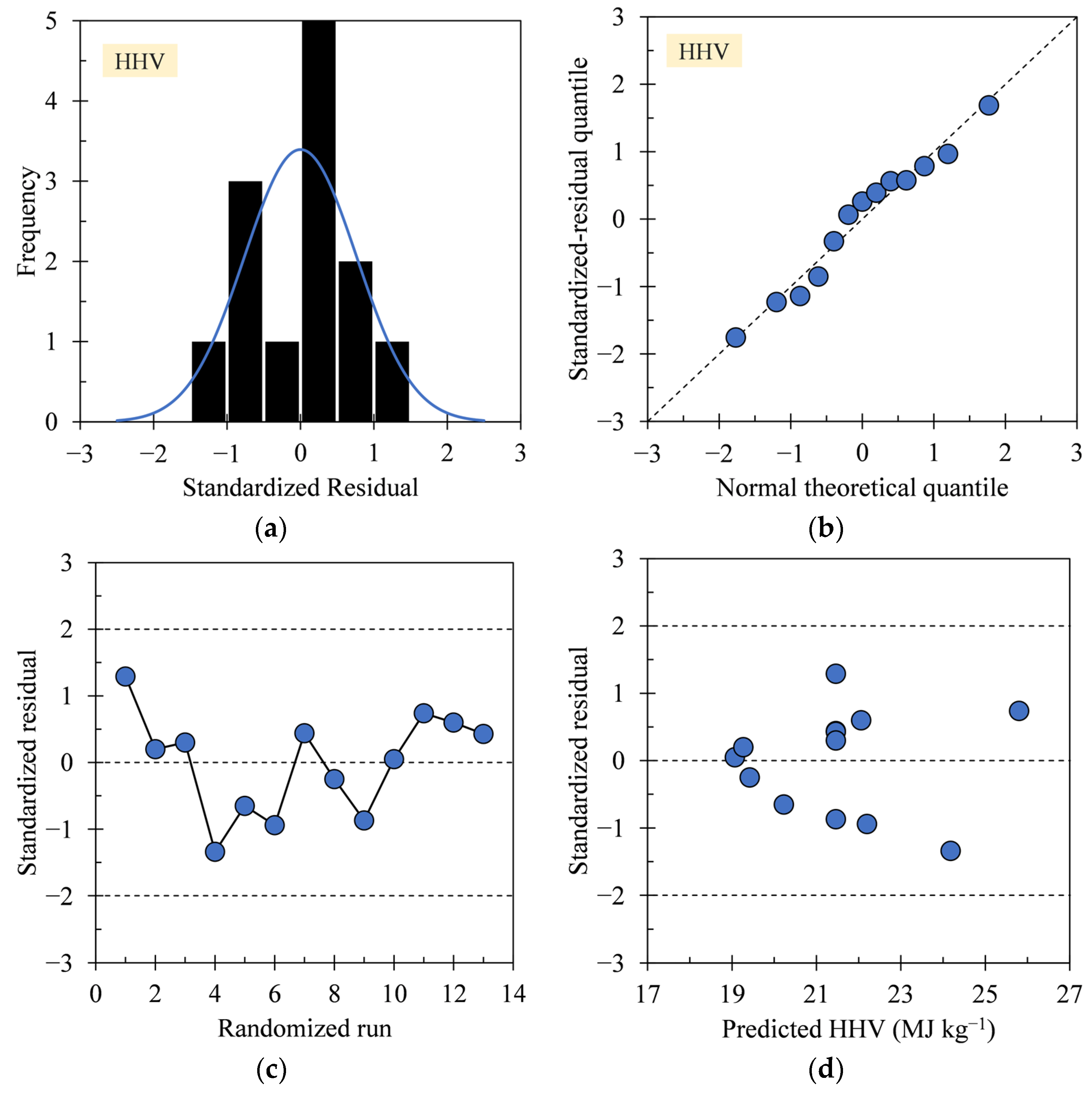
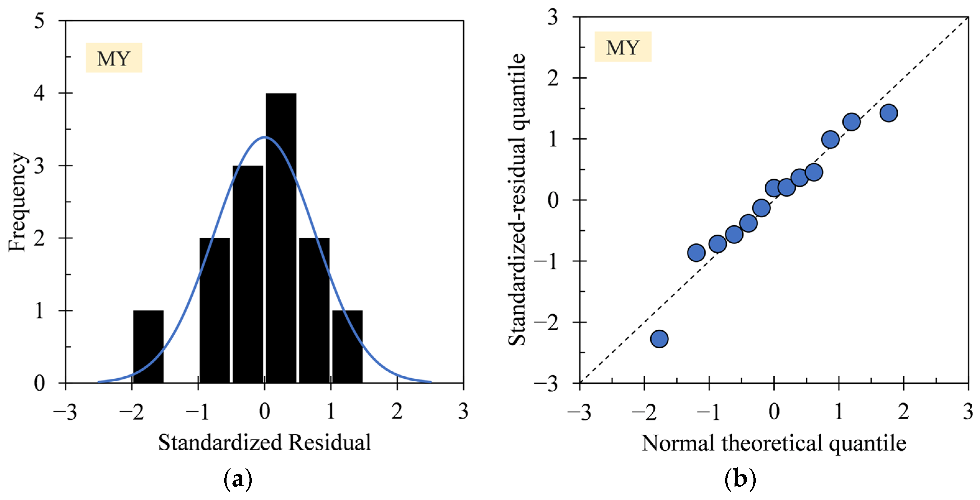
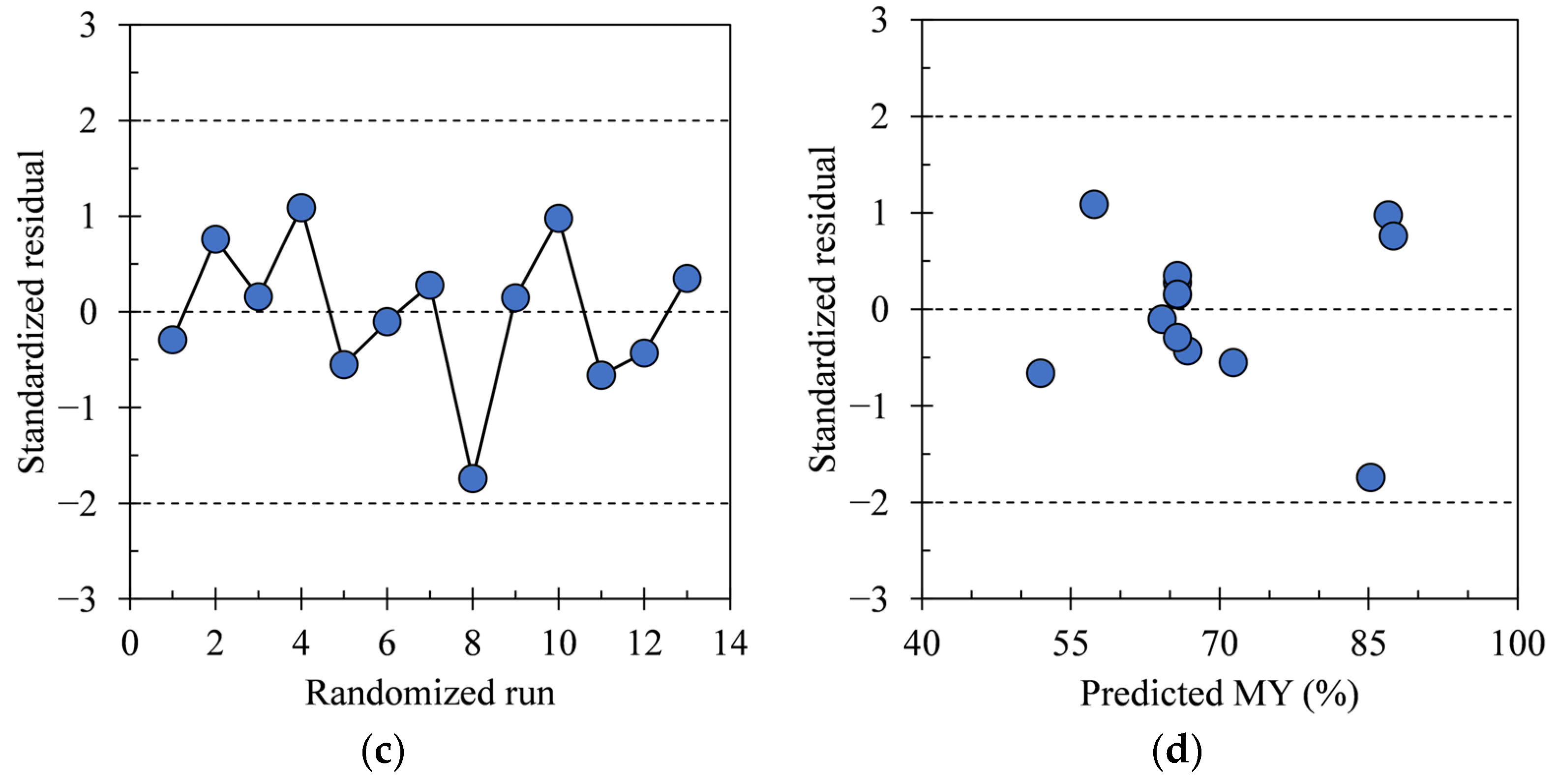
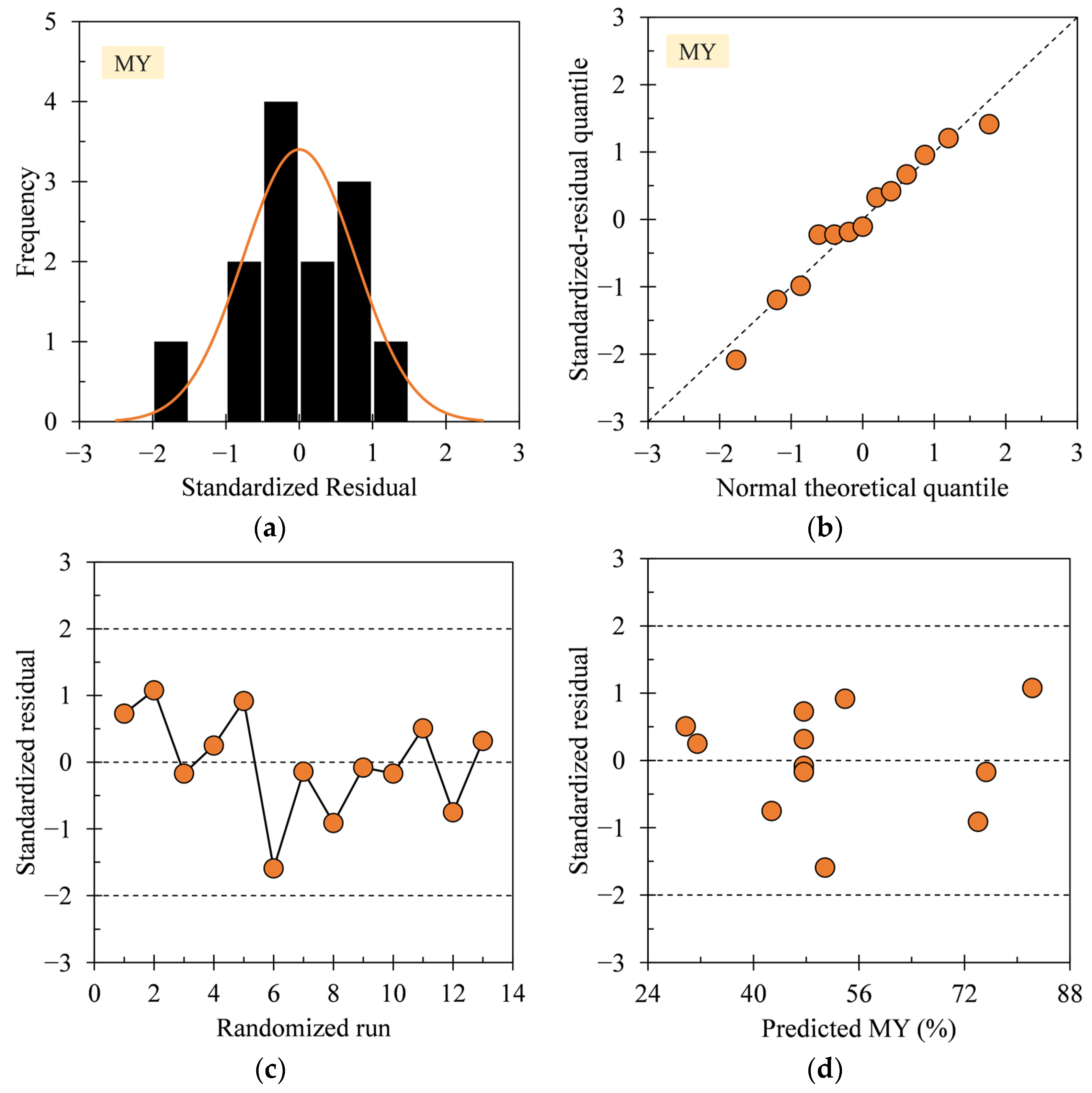
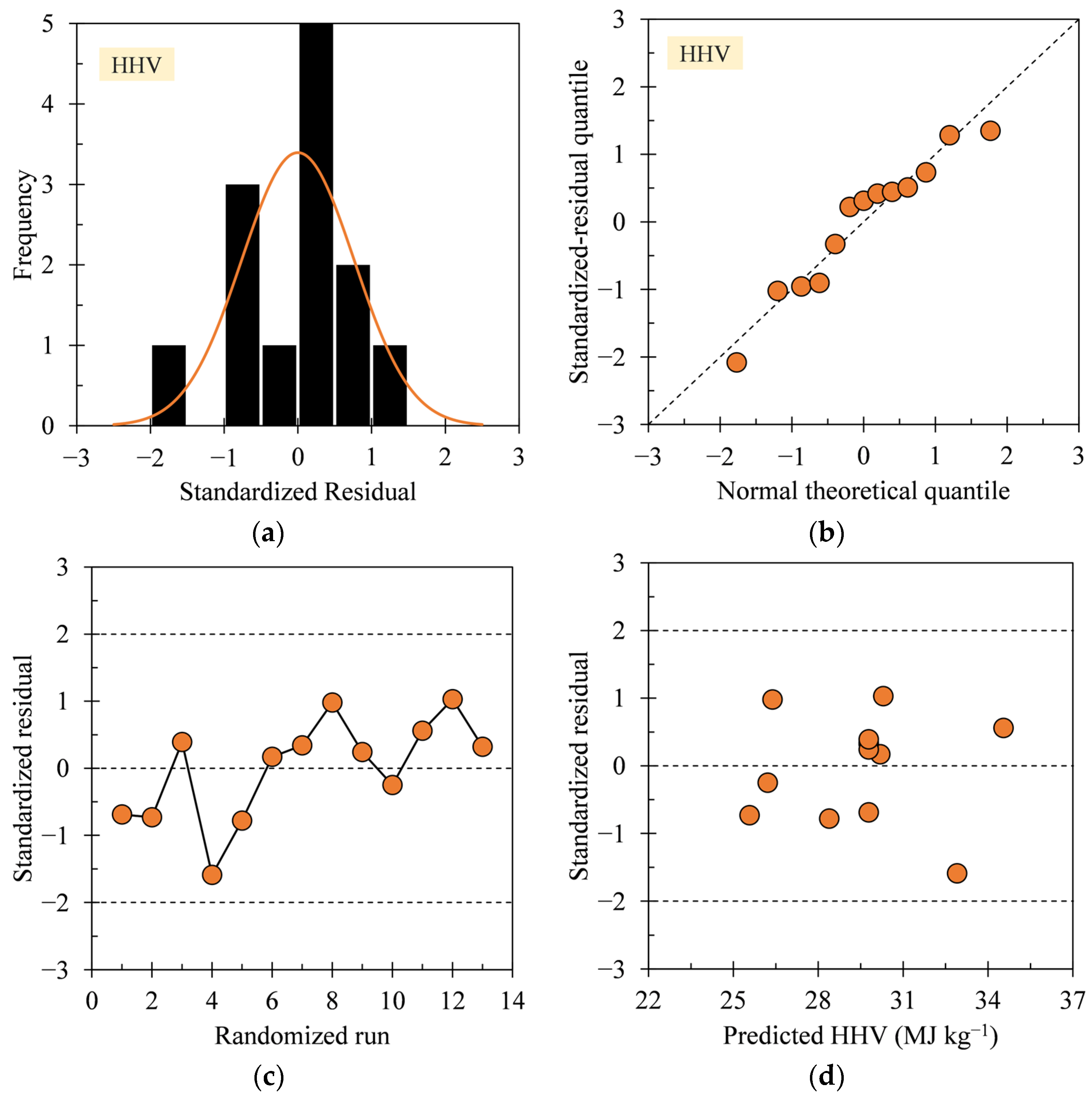
3.1. Regression Model Diagnosis

The goodness of fit and the regression significance of the overall models were assessed by the ANOVA global test, as shown in Table 4. Based on the R2 results, approximately 95.0–99.5% of the variance in all response models could be explained by the temperature and residence time of HTC, regardless of biomass type. The adequacy was confirmed by the corresponding F-ratios of much greater than 1. Concerning the null hypothesis (βi = βij = βii = 0) versus the alternative hypothesis (at least one β is non-zero), all p-values of the response models provided evidence of 0.00, meaning that the null hypothesis was rejected. These findings suggest that all regression models fitted the data points significantly and had at least one non-zero estimated coefficient [24,29]. In addition, the least coefficients were evidenced to meet the assumption of being specified in a linear way by having significant p-values of 0.00 for all linear systems (see Table 5) [24].
Graphical residual analysis was conducted to detect any potential issues in the regression assumptions, as exemplified in Figure 4. The HHV response of SB hydrochars was used as a representative for diagnosis (see Appendix A Figure A3, Figure A4 and Figure A5 for the other MY and HHV responses). The histogram in Figure 4a demonstrates a more or less bell-shaped distribution, confirming the normal distribution of random errors and a strong deterministic relationship. Thus, the mean error term (ε) was assumed to be zero, albeit not perfect. The histogram result corresponded to the reasonably clear linear pattern on the normal Q-Q plot without severe skewness and tail (see Figure 4b) [15,24]. Meanwhile, the run sequence plot in Figure 4c indicates no violation of the independent error assumption (having no auto-correlation), which is characterized by the points of standardized residuals overlapping the zero line repeatedly across the randomized runs. Consequently, the response model can avoid misleading due to over-optimistic predictions [30]. The scatter plot in Figure 4d shows the points of the standardized residuals against the predicted responses, which spread randomly around the zero line and form an unsystematic pattern. The result agrees with the assumption of homoscedasticity that the model had constant error variance and sufficient constituent factors [15,30]. Additionally, no red warning flags of outliers were found beyond the conservative cutoff of standardized residuals by ±2 [31], as illustrated in Figure 4c,d. The satisfaction for outliers reflects the absence of issues due to measurement variability or experimental error. Overall, since the other response models had relatively similar graphical tendencies and complied with the three residual assumptions, the factor coefficients in each model are sufficient to explain responses without causing appreciable residuals.
In detecting multicollinearity among the factor sets, variance inflation factors (VIFs) were assigned and found to converge around 1 (see Table 4), which were much smaller than the rule of thumb of 10, indicating the absence of multicollinearity [29]. This implies that the temperature and residence time did not determine each other (uncorrelated), and the effects of their factor systems were not confounded. Hence, all response models are reliable in terms of further interpretability concerning the significance masking [24,29].

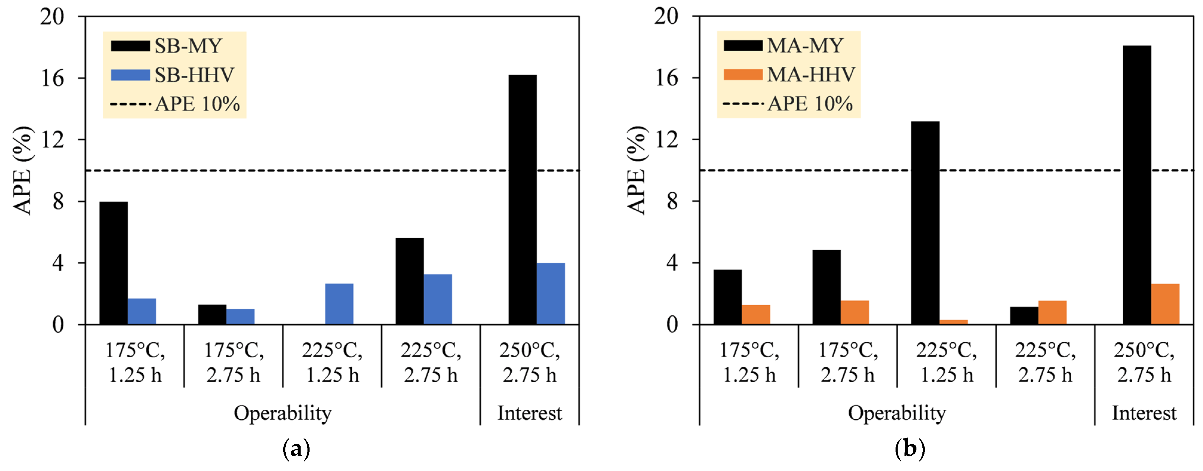
3.2. Data Validation

The new datasets for validation are listed in Table 6. Data points, which were distributed in different domains, give insight into the extent to which the models can be safely interpreted and optimized. The accuracy rating for the mean absolute percentage error (MAPE) was compared equivalently to the resulting APE scores, whose categories are divided into highly accurate (<10%), good (10–20%), reasonable (20–50%), and inaccurate (>50%), as proposed by Lewis [32]. In this study, an error percentage greater than 10% was designated as a red flag for the corresponding domain to be considered unsafe for interpretation and optimization. Figure 5 exhibits that almost all APEs were categorized as having high accuracy in the domain of operability, indicating that the domain is safe for interpreting the MY and HHV surface plots and optimizing the HTC operating parameters therein. The APE gave errors between 0.05 and 7.97% for MY (except one point belonging to MA; 13.17%) and 0.30 and 3.27% for HHV, regardless of biomass type. On the other hand, the domain of interest is indicated to be only reliable for interpreting and optimizing the HHV response, which also suggests that the optimization by HHV can be applied in all experimental domains. This was supported by the APEs of HHV, which showed 4.00% (SB) and 2.65% (MA) and were categorized as high accuracy, unlike those of the MY response, scoring above the threshold at 16.21% and 18.08%.

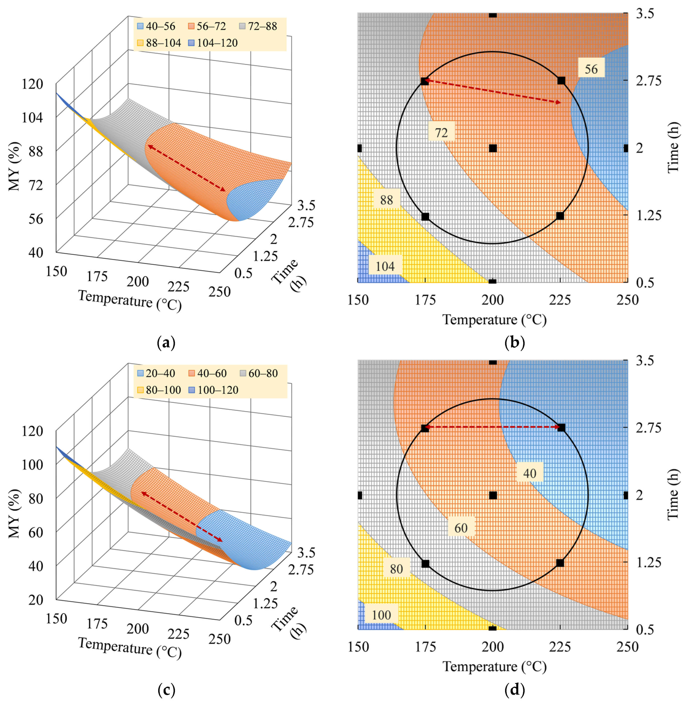
3.3. Interpretation of MY Model

Two- and three-dimensional surface plots of MY are depicted for SB and MA hydrochars in Figure 6. Both plots were proposed according to Equations (12) and (13). The recoverable solids of both hydrochars were observed to decrease as the temperature and time of HTC increased. The trends conformed to the significant antagonistic effects of all linear systems that had p-values of 0.00 and negatively signed coefficients (−β1 and −β2) (see Table 5). Such changes affirm the clear contribution of hydrous degradation through promoting ionic reactions and lowering water viscosity, particularly by temperature, since reactions due to residence time alone remain unclear [33,34]. In proportion to the coefficient magnitude, MA hydrochars presented lower yields of about 20–80% compared to SB at 40–88% in the domain of operability. This implies that fewer solids can be further utilized from MA as a fuel feedstock. Reasonably, proteins and lipids, which are abundant in NLBM, were reported to depend on other contents in reconstituting the solids, as opposed to holocellulose and lignin in LBM [35,36]. The amorphous structure of NLBM might also favor the susceptibility of MA to thermal degradation [37].
The local minima of SB and MA hydrochars appeared around a residence time of 2.75 h in the domain of operability from the concave-up curvatures, as depicted by the red dashed lines. The states were associated with the significant synergistic effects of the time-related quadratic systems (p-values of β22 = 0.00). Thereby, more solids survived above this time period at a given temperature. This phenomenon could be explained by the ongoing polymerization of soluble compounds in the aqueous phase, eventually leading to the precipitation of insoluble solids [34]. The highest increment was predicted to be 8% (SB) and 5% (MA) when the data were extended beyond the domain of operability.
Although not clearly visible due to the insignificance, the residence time of local minima decreased as the temperature increased. The time shift from 2.75 to 2.50 h was slightly more prominent in the SB plot when the temperature ranged between 175 °C and 225 °C, compared to the MA, which was steady at around 2.75 h. This tendency agrees with the smaller p-value of the SB interaction system (p-values of β12 = 0.32, 0.90), rendering the SB plot slightly twisted. The saturation of free radicals probably affected the condensation–polymerization of SB-soluble fragments at low temperatures, thus requiring a longer reaction time to precipitate [34].
M Y S B = 65.76 8.76 x 1 5.18 x 2 + 0.93 x 1   2 + 2.84 x 2   2 + 1.75 x 1 x 2 ,
M Y M A = 47.63 11.39 x 1 9.89 x 2 + 1.21 x 1   2 + 3.72 x 2   2 + 0.20 x 1 x 2 ,

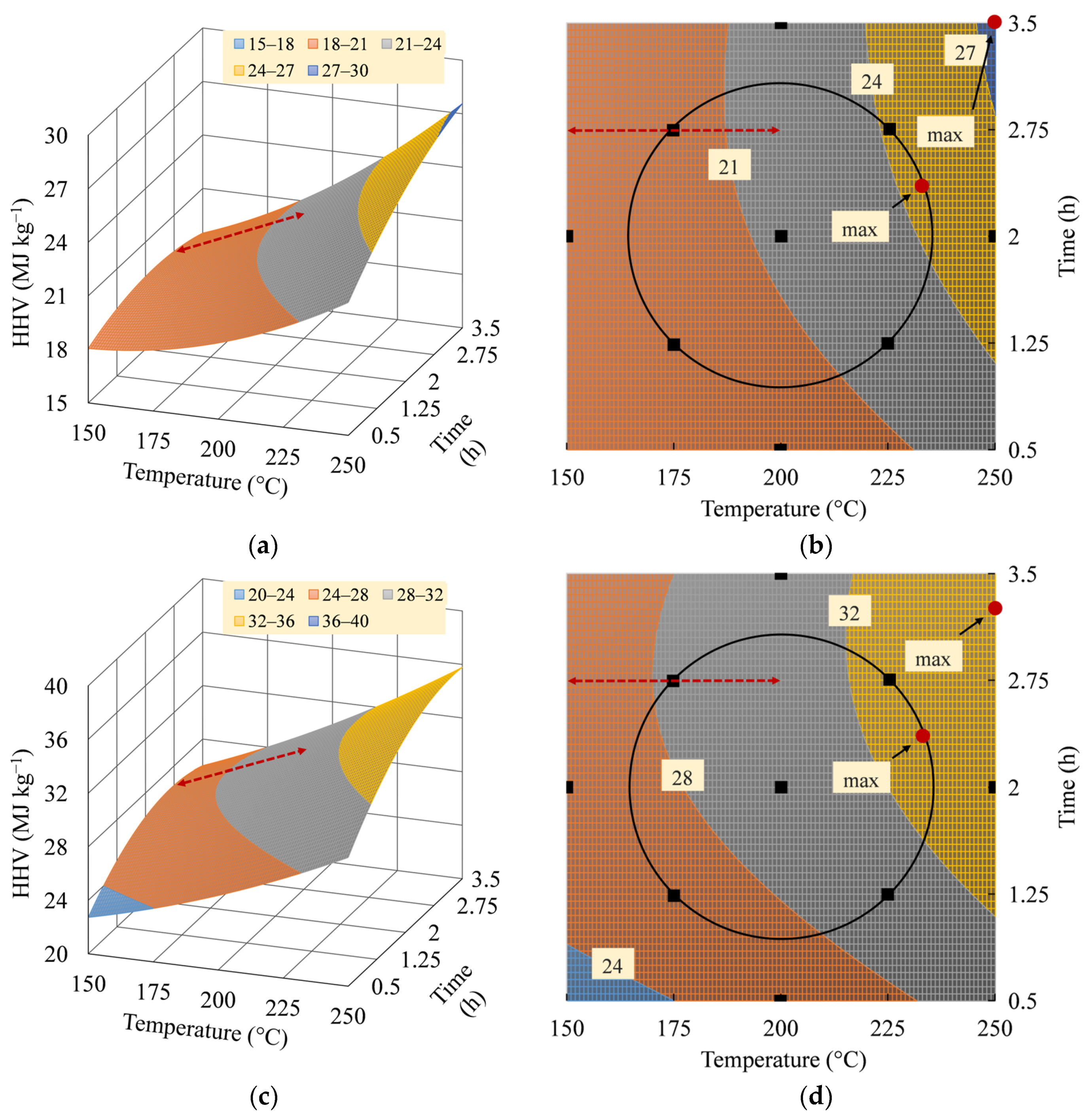
3.4. Interpretation of HHV Model

Two- and three-dimensional surface plots of HHV are shown in Figure 7 for SB and MA hydrochars, respectively. The regression functions are expressed in Equations (14) and (15). The heating values of both hydrochars showed monotonic trends that increased along with temperature and residence time. The trends were a consequence of the significant synergistic effects of the linear systems (p-values of β1 and β2 = 0.00) (see Table 5). Carbon enrichment widely explained the increase in HHV through deoxygenation reactions such as dehydration and decarboxylation [38,39]. Consistent with the resulting coefficient magnitude, MA hydrochars exhibited heating values about 30% greater than SB. The HHV ranged from 24 to 36 (MA) and 18 to 27 MJ kg−1 (SB) within the domain of interest. The higher heat that could be released by MA hydrochars indicates a potential for broader fuel applications. The difference in HHV between the two hydrochars could be also partly caused by the chemical structures of the hydrocarbons formed. The open-chain structures, carbon chain length, carbon saturation, and amorphicity were reported to facilitate higher heat release, as compared to their counterpart structures [40,41,42].
Noticeably, the quadratic systems in the HHV responses showed significant synergistic and antagonistic effects in relation to temperature and residence time (p-values of β11 = 0.01 (SB), 0.02 (MA); p-values of −β22 = 0.03, 0.00), respectively. Although the turning points of the concave-down curvatures were faint for both hydrochars, the local maxima appeared around 2.75 h, as depicted by the red dashed lines. Retention with longer times resulted in a slight decrease in HHV of less than 1 MJ kg−1. Nevertheless, the attenuation of HHV disappeared progressively with carbon enrichment above 200 °C. The decrease in heating value might be owing to the deposition of oxygenated functional groups during partial hydrolysis at lower temperatures and higher residence times [13,43].
Unfortunately, the interaction effects of temperature and time on the local maxima could not be further observed regarding the insignificant p-values of 0.14 (SB) and 0.18 (MA) and the disappearance of the local peaks at higher temperatures. This infers that the carbonization reaction, which was particularly induced by temperature, prevailed in compensating for the adverse effects of oxygen deposition on HHV.
H H V S B = 21.46 + 1.68 x 1 + 0.70 x 2 + 0.24 x 1   2 0.20 x 2   2 + 0.29 x 1 x 2 ,
H H V M A = 29.78 + 2.08 x 1 + 1.18 x 2 + 0.15 x 1   2 0.46 x 2   2 + 0.18 x 1 x 2

3.5. Optimum Operating Parameters

Based on visual inspection of Figure 7, the HHV surface plots of the SB and MA hydrochars display a rising-ridge surface, implying that the global maxima or minima were beyond the domain of interest (–2 ≤ x1,2 ≤ 2) [15,16]. They were evidenced by the critical coordinates of the first derivative, which were located at (–3.17, –0.55) and (–6.89, –0.07), respectively. The negative coordinates corresponding to the global minima also did not satisfy the optimization requirement of maximum output. Therefore, the HHV was then maximized and governed locally in the domain of operability and interest.
By implementing the Lagrange multiplier method, the optimum operating parameters in the domain of operability were found to be almost the same for SB and MA hydrochars, which were around 233 °C for 2.4 h (see Table 7). They were predicted to possess maximum HHVs of 24.61 and 33.39 MJ kg−1, as denoted by the red dots inside the circular boundary in Figure 7. The optimum conditions were observed to vary when the optimization was extended to the domain of interest. Using the single-variable method, the maximum HHVs of SB and MA hydrochars were predicted to be 27.54 and 35.83 MJ kg−1, as shown by the red dots between the square and circular boundaries. Both were achieved at the most severe temperature of 250 °C, while their residence times were different at 3.50 and 3.25 h, respectively.

4. Conclusions

The significance and optimization of temperature and residence time were successfully investigated for the HTC of SB and MA. The MY and HHV responses of hydrochars were modeled using the RSM–CCD method. Diagnosis of the regression models revealed a good fulfillment of the goodness of fit, regression assumptions, and multicollinearity. Temperature and time were estimated to significantly control the hydrothermal process (p-values = 0.00–0.03), particularly in their linear and quadratic systems. Both operating parameters showed antagonistic and synergistic relationships with the MY and HHV, respectively. Holistically, under the whole experimental domain, the optimum operating parameters for HTC of SB and MA were reliably achieved at the most severe temperature of 250 °C, with different residence times of 3.5 and 3.25 h. The respective HHV was predicted to be maximized at 27.54 and 35.83 MJ kg−1.

Author Contributions

Conceptualization, N.L. and K.T.; methodology, N.L.; software, N.L. and K.T.; validation, N.L., T.F. and K.T.; formal analysis, N.L.; investigation, N.L.; resources, K.T.; data curation, N.L.; writing—original draft preparation, N.L.; writing—review and editing, K.T.; visualization, N.L.; supervision, T.F., X.W. and K.T.; project administration, K.T.; funding acquisition, K.T. All authors have read and agreed to the published version of the manuscript.

Funding

This research was funded by the Japan Society for the Promotion of Science (JSPS) under the Grants-in-Aid for Scientific Research (KAKENHI) program, grant number JP22K05905.

Data Availability Statement

All data used are referenced and are available within the manuscript and the Appendix A.

Conflicts of Interest

The authors declare no conflicts of interest.

Appendix A

Figure A1. A visual depiction of the two-factor CCD model for determination of total runs, with the least 5 center replications.
Thermo 04 00007 g0a1
Figure A2. Diagram of determining the new datasets, cross-referenced with Fakkaew et al. [44].
Thermo 04 00007 g0a2
Figure A3. Graphical residual analysis for the MY response of SB hydrochars. (a) Histogram; (b) Normal Q-Q plot; (c) Run sequence plot; (d) Scatter plot.
Thermo 04 00007 g0a3aThermo 04 00007 g0a3b
Figure A4. Graphical residual analysis for the MY response of MA hydrochars. (a) Histogram; (b) Normal Q-Q plot; (c) Run sequence plot; (d) Scatter plot.
Thermo 04 00007 g0a4
Figure A5. Graphical residual analysis for the HHV response of MA hydrochars. (a) Histogram; (b) Normal Q-Q plot; (c) Run sequence plot; (d) Scatter plot.
Thermo 04 00007 g0a5

References

  1. Wang, T.; Zhai, Y.; Zhu, Y.; Li, C.; Zeng, G. A review of hydrothermal carbonization of biomass waste for hydrochar formation: Process conditions, fundamentals, and physicochemical properties. Renew. Sustain. Energy Rev. 2018, 90, 223–247. [Google Scholar] [CrossRef]
  2. Kannan, S.; Gariepy, Y.; Raghavan, G.S.V. Optimization and characterization of hydrochar produced from microwave hydrothermal carbonization of fish waste. Waste Manag. 2017, 65, 159–168. [Google Scholar] [CrossRef] [PubMed]
  3. Boutaieb, M.; Guiza, M.; Roman, S.; Cano, B.L.; Nogales, S.; Ouderni, A. Hydrothermal carbonization as a preliminary step to pine cone pyrolysis for bioenergy production. C. R. Chim. 2020, 23, 607–621. [Google Scholar] [CrossRef]
  4. Shen, Y. A review on hydrothermal carbonization of biomass and plastic waste to energy products. Biomass Bioenergy 2020, 134, 105479. [Google Scholar] [CrossRef]
  5. Zhang, L.; Liu, S.; Wang, B.; Wang, Q.; Yang, G.; Chen, J. Effect of residence time on hydrothermal carbonization of corn cob residual. BioResources 2015, 10, 3979–3986. [Google Scholar] [CrossRef]
  6. Savage, P.E. Organic chemical reactions in supercritical water. Chem. Rev. 1999, 99, 603–622. [Google Scholar] [CrossRef]
  7. Perez, D.L.; Mayanga, P.C.T.; Abaide, E.R.; Zabot, G.L.; Castilhos, F.D. Hydrothermal carbonization and liquefaction: Differences, progress, challenges, and opportunities. Bioresour. Technol. 2022, 343, 126084. [Google Scholar]
  8. Cao, Z.; Hulsemann, B.; Wust, D.; Oechsner, H.; Lautenbach, A.; Kruse, A. Effect of residence time during hydrothermal carbonization of biogas digestate on the combustion characteristics of hydrochar and the biogas production of process water. Bioresour. Technol. 2021, 333, 125110. [Google Scholar] [CrossRef]
  9. Mariyam, S.; Alherbawi, M.; Pradhan, S.; Al-Ansari, T.; McKay, G. Biochar yield prediction using response surface methodology: Effect of fixed carbon and pyrolysis operating conditions. Biomass Convers. Biorefin. 2023, 2023, 1–14. [Google Scholar] [CrossRef]
  10. Xing, J.; Luo, K.; Wang, H.; Gao, Z.; Fan, J. A comprehensive study on estimating higher heating value of biomass from proximate and ultimate analysis with machine learning approaches. Energy 2019, 188, 116077. [Google Scholar] [CrossRef]
  11. McKendry, P. Energy production from biomass (part 1): Overview of biomass. Bioresour. Technol. 2002, 83, 37–46. [Google Scholar] [CrossRef] [PubMed]
  12. Prins, M.J.; Ptasinski, K.J.; Janssen, F.J.J.G. From coal to biomass gasification: Comparison of thermodynamic efficiency. Energy 2007, 32, 1248–1259. [Google Scholar] [CrossRef]
  13. Tahir, M.H.; Zhao, Z.; Ren, J.; Naqvi, M.; Ahmed, M.S.; Shah, T.U.H.; Shen, B.; Elkamel, A.; Irfan, R.M.; Rahman, A.U. Fundamental investigation of the effect of functional groups on the variations of higher heating value. Fuel 2019, 253, 881–886. [Google Scholar] [CrossRef]
  14. Khunphakdee, P.; Korkerd, K.; Soanuch, C.; Chalermsinsuwan, B. Data-driven correlations of higher heating value for biomass, waste and their combination based on their elemental compositions. Energy Rep. 2022, 8, 36–42. [Google Scholar] [CrossRef]
  15. Trutna, L.; Spagon, P.; Castillo, E.D.; Moore, T.; Hartley, S.; Hurwitz, A. Chapter 5: Process improvement. In NIST/SEMATECH Engineering Statistics Handbook; Tobias, P., Trutna, L., Eds.; National Institute of Standards and Technology: Gaithersburg, MD, USA, 2003. [Google Scholar]
  16. Bezerra, M.A.; Santelli, R.E.; Oliveira, E.P.; Villar, L.S.; Escaleira, L.A. Response surface methodology (RSM) as a tool for optimization in analytical chemistry. Talanta 2008, 76, 965–977. [Google Scholar] [CrossRef]
  17. Sahoo, P.; Barman, T.K. 5—ANN modelling of fractal dimension in machining. In Mechatronics and Manufacturing Engineering; Davim, J.P., Ed.; Woodhead Publishing: Cambridge, UK, 2012; pp. 159–226. [Google Scholar]
  18. Arif, A.B.; Budiyanto, A.; Diyono, W.; Hayuningtyas, M.; Marwati, T.; Sasmitaloka, K.S.; Richana, N. Bioethanol production from sweet sorghum bagasse through enzymatic process. IOP Conf. Ser. Earth Environ. Sci. 2019, 309, 012033. [Google Scholar] [CrossRef]
  19. Wahyono, T.; Firsoni, F. The changes of nutrient composition and in vitro evaluation on gamma irradiated sweet sorghum bagasse. Sci. J. Appl. Isot. Radiat. 2016, 12, 69–77. [Google Scholar] [CrossRef]
  20. Cabrita, A.R.J.; Fernandes, J.G.; Valente, I.M.; Almeida, A.; Lima, S.A.C.; Fonseca, A.J.M.; Maia, M.R.G. Nutritional composition and untargeted metabolomics reveal the potential of Tetradesmus obliquus, Chlorella vulgaris and Nannochloropsis oceanica as valuable nutrient sources for dogs. Animals 2022, 12, 2643. [Google Scholar] [CrossRef]
  21. Coelho, D.; Pestana, J.; Almeida, J.M.; Alfaia, C.M.; Fontes, C.M.G.A.; Moreira, O.; Prates, J.A.M. A high dietary incorporation level of Chlorella vulgaris improves the nutritional value of pork fat without impairing the performance of finishing pigs. Animals 2020, 10, 2384. [Google Scholar] [CrossRef]
  22. Queiroz, V.A.V.; Silva, C.S.D.; Menezes, C.B.D.; Schaffert, R.E.; Guimaraes, F.F.M.; Guimaraes, L.J.M.; Guimaraes, P.E.D.P.; Tardin, F.D. Nutritional composition of sorghum [Sorghum biocolor (L.) Moench] genotypes cultivated without and with water stress. J. Cereal Sci. 2015, 65, 103–111. [Google Scholar] [CrossRef]
  23. Gaxiola, J.E.B.; Ross, A.B.; Dupont, V. Multi-variate and multi-response analysis of hydrothermal carbonization of food waste: Hydrochar composition and solid fuel characteristics. Energies 2022, 15, 5342. [Google Scholar] [CrossRef]
  24. Sarstedt, M.; Mooi, E. Regression analysis. In A Concise Guide to Market Research; Springer: Berlin, Germany, 2014; pp. 193–233. [Google Scholar]
  25. Kim, S.; Kim, H. A new metric of absolute percentage error for intermittent demand forecasts. Int. J. Forecast. 2016, 32, 669–679. [Google Scholar] [CrossRef]
  26. Chicco, D.; Warrens, M.J.; Jurman, G. The coefficient of determination R-squared is more informative than SMAPE, MAE, MAPE, MSE and RMSE in regression analysis evaluation. Peer J. Comput. Sci. 2021, 7, e623. [Google Scholar] [CrossRef]
  27. University of Texas. Available online: https://web.ma.utexas.edu/users/m408m/Display14-8.shtml (accessed on 25 December 2022).
  28. Vadlamani, S.K.; Xiao, T.P.; Yablonovitch, E. Physics successfully implements Lagrange multiplier optimization. Proc. Natl. Acad. Sci. USA 2020, 117, 26639–26650. [Google Scholar] [CrossRef] [PubMed]
  29. Forthofer, R.N.; Lee, E.S.; Hernandez, M. 13–Linear regression. In Biostatistics, 2nd ed.; Forthofer, R.N., Lee, E.S., Hernandez, M., Eds.; Academic Press: Burlington, NJ, USA, 2007; pp. 349–386. [Google Scholar]
  30. Yang, H. Visual assessment of residual plots in multiple linear regression: A model-based simulation perspective. Mult. Linear Regres. Viewp. 2012, 38, 24–37. [Google Scholar]
  31. Eric, S. An introduction to graphical analysis of residual scores and outlier detection in bivariate least squares regression analysis. In Proceedings of the Annual Meeting of the Southwest Educational Research Association, New Orleans, LA, USA, 25 January 1996. [Google Scholar]
  32. Lewis, C.D. Industrial and Business Forecasting Methods: A Practical Guide to Exponential Smoothing and Curve Fitting; Butterworth Scientific: London, UK, 1982. [Google Scholar]
  33. Moller, M.; Nilges, P.; Harnisch, F.; Schroder, U. Subcritical water as reaction environment: Fundamentals of hydrothermal biomass transformation. ChemSusChem 2011, 4, 566–579. [Google Scholar] [CrossRef]
  34. Funke, A.; Ziegler, F. Hydrothermal carbonization of biomass: A summary and discussion of chemical mechanism for process engineering. Biofuels Bioprod. Biorefin. 2010, 4, 160–177. [Google Scholar] [CrossRef]
  35. Li, Y.; Liu, H.; Xiao, K.; Liu, X.; Hu, H.; Li, X.; Yao, H. Correlations between the physicochemical properties of hydrochar and specific components of waste lettuce: Influence of moisture, carbohydrates, proteins, and lipids. Bioresour. Technol. 2019, 272, 482–488. [Google Scholar] [CrossRef]
  36. Xiao, K.; Liu, H.; Li, Y.; Yi, L.; Zhang, X.; Hu, H.; Yao, H. Correlations between hydrochar properties and chemical constitution of orange peel waste during hydrothermal carbonization. Bioresour. Technol. 2018, 265, 432–436. [Google Scholar] [CrossRef]
  37. Zhuang, X.; Zhan, H.; Song, Y.; He, C.; Huang, Y.; Yin, X.; Wu, C. Insights into the evolution of chemical structures in lignocellulose and non-lignocellulose biowastes during hydrothermal carbonization (HTC). Fuel 2019, 236, 960–974. [Google Scholar] [CrossRef]
  38. Saha, S.; Islam, M.T.; Calhoun, J.; Reza, T. Effect of hydrothermal carbonization on fuel and combustion properties of shrimp shell waste. Energies 2023, 16, 5534. [Google Scholar] [CrossRef]
  39. Smith, A.M.; Singh, S.; Ross, A.B. Fate of inorganic material during hydrothermal carbonisation of biomass: Influence of feedstock on combustion behaviour of hydrochar. Fuel 2016, 169, 135–145. [Google Scholar] [CrossRef]
  40. Demirbas, A.; Al-Ghamdi, K. Relationships between specific gravities and higher heating values of petroleum components. Pet. Sci. Technol. 2015, 33, 732–740. [Google Scholar] [CrossRef]
  41. Sarikoc, S. Fuels of the diesel-gasoline engines and their properties. In Diesel and Gasoline Engines; Viskup, R., Ed.; IntechOpen: London, UK, 2020. [Google Scholar]
  42. Gong, C.; Huang, J.; Feng, C.; Wang, G.; Tabil, L.; Wang, D. Effects and mechanism of ball milling on torrefaction of pine sawdust. Bioresour. Technol. 2016, 214, 242–247. [Google Scholar] [CrossRef] [PubMed]
  43. Jain, A.; Balasubramanian, R.; Srinivasan, M.P. Hydrothermal conversion of biomass waste to activated carbon with high porosity: A review. Chem. Eng. J. 2016, 283, 789–805. [Google Scholar] [CrossRef]
  44. Fakkaew, K.; Koottatep, T.; Polprasert, C. Effects of hydrolysis and carbonization reactions on hydrochar production. Bioresour. Technol. 2015, 192, 328–334. [Google Scholar] [CrossRef]
Figure 1. Schematic of hydrochar production. (a) Blending dried biomasses and deionized water in PTFE liner; (b) Activating HTC by inducting vessels thermally; (c) Separating slurry by filter paper before proceeding with final drying.
Thermo 04 00007 g001
Figure 2. The appearance of SB (right) and MA (left) biomasses and representative hydrochars. (a) Raw state; (b) 175 °C and 2.75 h (CCD dataset); (c) 250 °C and 2.75 h (validation dataset).
Thermo 04 00007 g002
Figure 3. Experimental domains of operability (circular) and interest (square) with their boundary functions.
Thermo 04 00007 g003
Figure 4. Graphical residual analysis for the HHV response of SB hydrochars. (a) Histogram; (b) Normal Q-Q plot; (c) Run sequence plot; (d) Scatter plot.
Thermo 04 00007 g004
Figure 5. APE scores of MY and HHV validation in each experimental domain. (a) SB hydrochars; (b) MA hydrochars.
Thermo 04 00007 g005
Figure 6. Descending-valley contour of MY: (a) 3D and (b) 2D plots of SB hydrochars; (c) 3D and (d) 2D plots of MA hydrochars.
Thermo 04 00007 g006
Figure 7. Raising-ridge contour of HHV: (a) 3D and (b) 2D plots of SB hydrochars; (c) 3D and (d) 2D plots of MA hydrochars.
Thermo 04 00007 g007
Table 1. Summary of the biochemical composition of SB and MA biomasses on a dry basis.
BiomassCarbohydrate (%) 1Protein (%)Lipid (%)Fiber (%) 2Ash (%)Reference
SB23.092.050.9063.930.11[18]
5.205.401.8579.108.45[19]
MA20.0243.909.7916.409.89[20]
35.6242.808.731.0511.80[21]
1 Carbohydrate (%) = 100% − Protein − Lipid − Fiber − Ash [22] (w/w in a dry matter basis). 2 Fiber (NDF) consists of lignin and non-starch carbohydrates, such as cellulose and hemicellulose.
Table 2. Factors and levels of hydrothermal carbonization experiments with CCD.
FactorSymbolCoded and Un-Coded Factor Level
−2 (−α)−1012 (α)
Temperature (°C)x1150175200225250
Residence time (h)x20.501.252.002.753.50
Table 3. Full-run experimental design and obtained responses.
Factor (x)Response (y)Remark
MY (%)HHV (MJ kg−1)
x1x2SBMASBMA
−1−179.4971.1319.3326.62Factorial point
1−163.8845.7821.8730.23Factorial point
−1169.5556.8220.0028.20Factorial point
1160.9432.2723.7132.53Factorial point
−2090.2374.7119.0926.15Axial point
2049.8031.3226.0634.68Axial point
0−289.9885.7519.3425.39Axial point
0265.3740.3422.2730.55Axial point
0066.6947.1821.6129.86Center point
0066.9148.6621.6129.86Center point
0066.2747.3721.1529.84Center point
0066.3047.0921.5729.87Center point
0064.8049.9721.9129.61Center point
Table 4. Summary of the regression models from ANOVA.
SourceResponse (y)F-Ratiop-ValueR2
SBMASBMASBMA
ModelMY26.4959.780.00 *0.00 *0.9500.977
HHV70.22261.730.00 *0.00 *0.9800.995
* shows statistical significance at p-value < 0.05 (confidence level of 95%).
Table 5. Coefficients and collinearities for each factor system of the response models.
Response (y)Factor SystemCoefficient (β)p-ValueCollinearity (VIF)
SBMASBMASBMA
MYInterceptβ0: 65.7647.630.00 *0.00 *
x1: Temperatureβ1: −8.76−11.390.00 *0.00 *1.001.00
x2: Timeβ2: −5.18−9.890.00 *0.00 *1.001.00
x12β11: 0.931.210.220.111.091.09
x22β22: 2.843.720.00 *0.00 *1.091.09
x1x2β12: 1.750.200.320.901.001.00
HHVIntercept21.4629.780.00 *0.00 *
x1: Temperature1.682.080.00 *0.00 *1.001.00
x2: Time0.701.180.00 *0.00 *1.001.00
x120.240.150.01 *0.02 *1.091.09
x22−0.20−0.460.03 *0.00 *1.091.09
x1x20.290.180.140.181.001.00
* shows statistical significance at p-value < 0.05 (confidence level of 95%).
Table 6. Observed and predicted results based on new datasets for validation.
SampleFactor (x)MY (%)HHV (MJ kg−1)Remark
x1x2ObservationPredictionObservationPrediction
SB−1−178.9385.2219.7519.41Operability
−1170.4471.3620.4420.23
1−164.1764.2021.6222.19
1160.7557.3423.4024.17
2145.7153.1227.9826.86Interest
MA−1−171.5174.0426.7326.39Operability
−1156.6053.8627.9628.39
1−144.9450.8630.2830.19
1131.1231.4832.4132.91
2129.2023.9236.5935.62Interest
Table 7. Optimum conditions for each domain based on the maximized HHV.
Factor and ResponseDomain of OperabilityDomain of Interest
SBMASBMA
Temperature (°C)233.24 (1.33) 1233.10 (1.32)250.00 (2.00)250.00 (2.00)
Residence time (h)2.36 (0.48)2.37 (0.50)3.50 (2.00)3.25 (1.67)
HHV (MJ kg−1)24.6133.3927.5435.83
1 Values in the subscript parentheses are coded temperatures and times.
Disclaimer/Publisher’s Note: The statements, opinions and data contained in all publications are solely those of the individual author(s) and contributor(s) and not of MDPI and/or the editor(s). MDPI and/or the editor(s) disclaim responsibility for any injury to people or property resulting from any ideas, methods, instructions or products referred to in the content.

