1. Introduction
DSC is a differential technique that measures the difference in heat flow rate between a pan containing a sample and an empty reference pan. It is assumed that the physical properties of the sample and reference pan are negligible, meaning that the measured heat flow is just the heat flow into the sample, which is reasonable if the weight and shape of the two pans are close to each other (see Experimental for discussion of what this means). DSC is used to measure the heat capacity of materials on a milligram scale (10–100 mg). However, DSC does not measure heat capacity directly, but rather uses the experimental sample mass, m (mg); measured heat flow, Δ
Q/Δ
t (J/s); and temperature change, T (°C or K), to calculate the specific heat capacity
cp, as shown in Equation (1).
As can be seen in Equation (1), the accuracy of the measurement requires the ability to accurately measure heat flow and heating rate. All DSC instruments use temperature sensors (thermocouple, thermopile, resistance thermometer, etc.) in contact with the sample pan to measure temperature. Because the temperature sensor is not in direct contact with the sample, the temperature calibration of the sensor is typically performed with melting point standards in the same type of pan and heating rate used for sample measurements. A reasonable assumption is that temperature control and measurement are accurate and reproducible during a series of experiments.
Deviations from the literature values in
cp using existing procedures generally fall in the range of ±2–5% [
1]. This means that there is an error of ±2–5% in the absolute value of the heat flow signal since a minimal amount of error can be attributed to the sensors or the differences in pans, given a properly functioning instrument and properly prepared samples, which crucially involves minimizing the difference in pan mass. The bulk of the error is caused by changes in the heat flow baseline over time (minutes to hours). These changes include:
Drift in the absolute value of the DSC heat flow signal;
Baseline slope (over a temperature range);
Curvature of the baseline (over a temperature range).
Currently, two very different approaches are used to minimize the effect of baseline drift in the DSC. These include the ASTM method and Modulated DSC (MDSC®). These methods are briefly discussed below and are followed by a detailed description/illustration of the proposed Heat–Cool method.
Possibly the most commonly used method for measuring heat capacities using DSC is outlined by the ASTM ( ASTM E1269-11 (2018)) [
2]. Due to baselines that are dependent on instrument design, the absolute value of the heat flow signal cannot be used outright, so the ASTM procedure corrects for this by performing a blank experiment prior to the experiment on the sample, with both experiments performed under the same conditions including heating rate. This changes Equation (1) to
While this improves results, calculated heat capacities are still not always highly accurate (agreeing with the literature). In order to correct for this, the current standard procedure adds a heat capacity calibration factor based on the heat capacity of a well-characterized material, often sapphire. The origin of this corrective factor is due to undetermined heat flow between the sample pan and the surroundings, including the purge gas and the cell walls. Using
D to denote the heat flow difference between the baseline measured in the blank and the sample (
s) or standard (
st), the final form of the heat capacity calculation becomes
The heat capacity of the standard for use in this equation is collected from the literature values. After the application of this correction, this procedure generally allows for deviations from the accepted literature values in the range of ±2–5%.
The major drawback of the ASTM method is that it requires three separate experiments. The first measurement is with empty pans to define the baseline of the DSC, the second measurement is with a sapphire disc of known mass for calibration, and the third measurement is with the material of interest. This is costly in terms of time and can introduce additional uncertainties. The highly sensitive nature of DSC means that even small details, such as the positioning of the pan in the DSC, can create detectable variability. When multiple experiments are used to calculate the heat capacity, such variability compounds limit the accuracy and precision of this procedure.
MDSC®
Modulated DSC was introduced in 1992 and immediately had an advantage over standard DSC because baseline artifacts such as drift, slope, and curvature had no effect on the measurement of heat capacity. MDSC
® eliminates the effect of baseline change by using the heat flow signal to calculate heat capacity. Instead of using the absolute value of the heat flow signal, MDSC
® uses the ratio of the change in heat flow (heat flow modulation amplitude,
Ampmhf) divided by the change in heating rate (modulated heating rate amplitude,
Ampmhr) to calculate
cp. Similar to the ASTM method, this ratio is multiplied by a calibration constant (
Kcp) obtained with sapphire or another heat capacity standard to obtain quantitative specific heat capacity
cp.
Heat–Cool DSC
We explore an alternative method that can obtain high accuracy data (agreeing with the literature) in a single experiment through the measurement of heat flow during one heating and cooling cycle. The central idea is that rather than performing a separate blank experiment to calculate the difference in heat flow between the blank and the sample, one can take the difference between the heat flow during heating and cooling of the same sample in the same experiment.
Here, qm is the normalized heat flow, the heat flow per sample mass.
In the case where the heating and cooling rates are the same but their signs are opposite gives
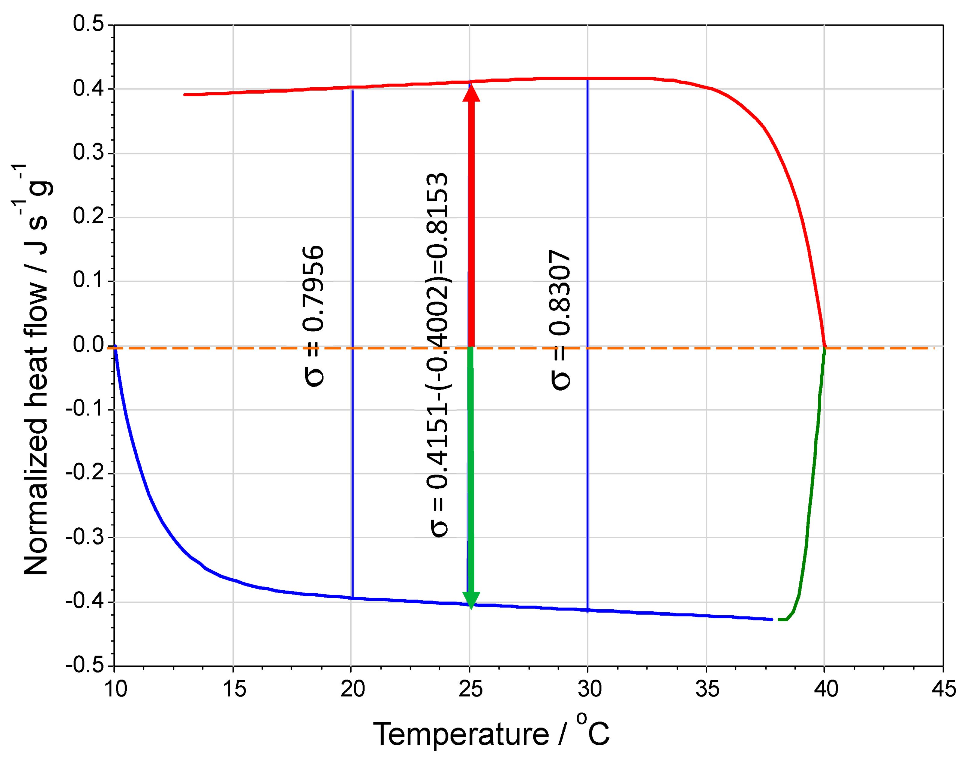
Here, σ has been defined as the difference in the normalized heating and cooling heat flows at the temperature of interest. It should be noted that the heat flow signals in the DSC are measured from the heat flow of zero (see Figure 2) and have opposite signs for heating and cooling, which leads to the addition of the two signals on subtraction.
The similarity of Equation (6) to Equation (2) reflects how both procedures perform some correction to account for the baseline behavior. However, one of the advantages of the Heat–Cool method is that it eliminates the need for the separate blank run, instead accounting for the effects of the baseline through measurements on only the sample.
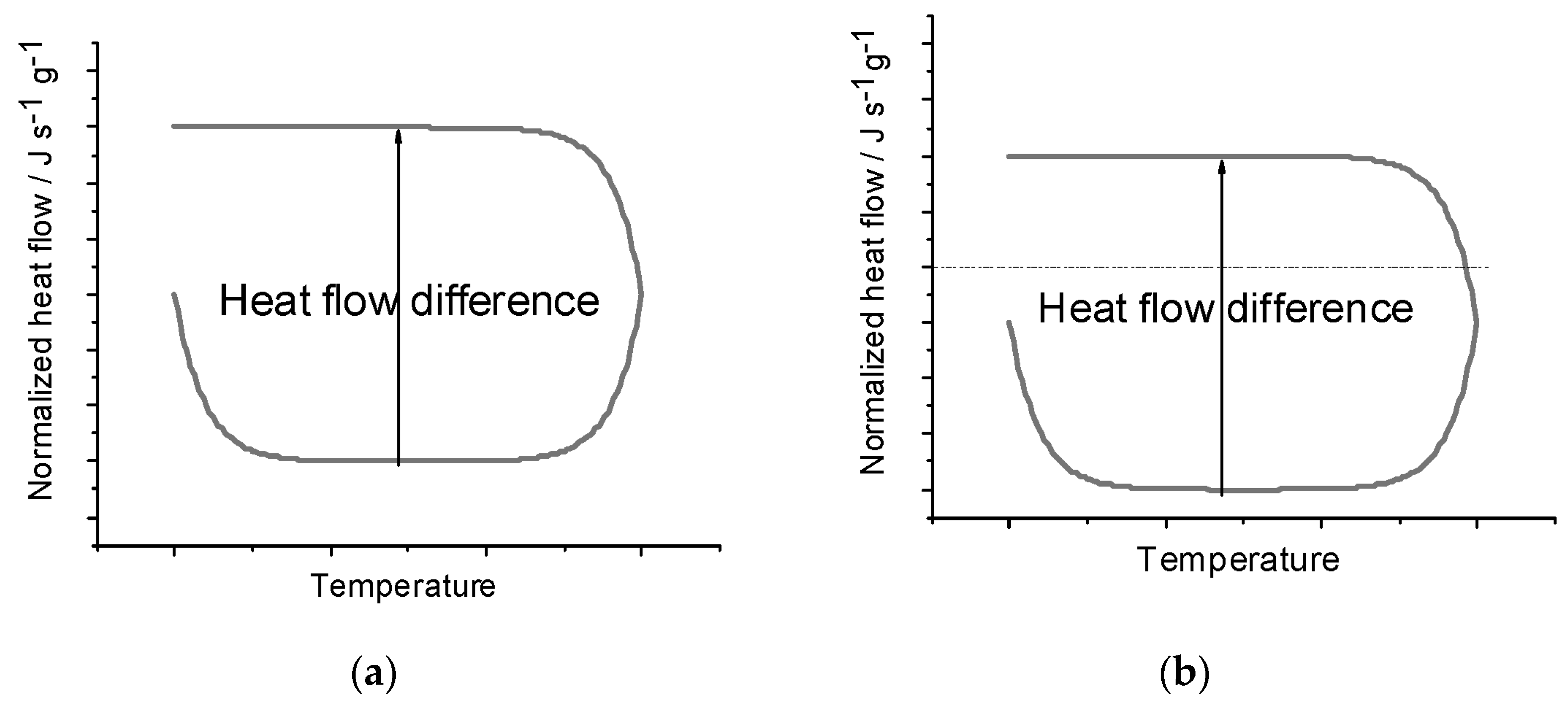
Figure 1a demonstrates what an ideal heating and cooling DSC curve would look like and how the heat flow difference is measured. Dividing the heat flow difference by the difference in the heating rates and the mass yields the specific heat capacity.
Figure 1b shows the same curve under the effects of a baseline shift and shows how the heat flow difference is unaffected. Since a constant baseline shift will shift both the heating and cooling curves in the same direction, the heat flow difference is unaffected, and thus, the heat capacity also is unaffected. Additionally, the Heat–Cool method outperforms the ASTM method by reducing the time to complete the experiment, which can consequently reduce uncertainty from longer timescale environmental shifts in the lab over the course of a day.
Schenker and Stager [
3] undertook a study to compare several dynamic methods to measure heat capacity: Modulated DSC (MDSC), dynamic DSC (DDSC), and steady-state DSC (SSADSC). Their use in a SSADSC experiment of a saw-tooth modulation, basically a heating–cooling cycle, yielded an expression for heat capacity that roughly mimics our Equation (5). However, as SSADSC is a modulated experiment, a variety of instrumental parameters have to be set to conduct the measurement. Determining the parameters requires additional effort compared to simply asking the instrument to run at fixed heating then cooling rates and measuring the heat flow signals obtained, as described in our Heat–Cool procedure. So, again, we hold that the use of the DSC in a normal manner, avoiding modulated techniques, is experimentally simpler.
In addition to conserving time through fewer experiments, the Heat–Cool method provides excellent accuracy, as discussed below. Like the ASTM and MDSC® methods, a heat capacity calibration constant/corrective factor could be used, but in our experience, under typical conditions, a Heat–Cool measurement differs from the literature values, generally under |2%| even without the extra correction. Such a corrective term might modestly improve measurements, though it would add additional sources of uncertainty and the measurement time required due to the additional experiment required. Consequently, a corrective term was not used for our measurements, and is not generally required for measurements.
Another benefit of the Heat–Cool method is that it provides an easy way to measure the heat capacity of a sample over a modest temperature range rather than at a single temperature. Over the course of a single experiment, the heat flow difference, and hence, in this case, the specific heat capacity, can be calculated at different temperatures, as seen in
Figure 2, allowing for the estimation of the temperature dependence of heat capacities of materials, at least over a modest temperature range. For liquids, there is a natural limiting range of temperatures for these measurements, and that results from the vapor pressure of liquid and the capacity of the sample pan to contain vapor loss as the vapor pressure of the liquid increases with temperature.
Materials table.
| | Water | Sapphire | Methanol | Ethanol | Propan-1-ol |
| Mole weight/g mol−1 | 18.02 | 101.96 | 32.04 | 46.069 | 60.10 |
| CAS # | 7732-18-5 | 1344-28-1 | 67-56-1 | 64-17-5 | 71-23-8 |
| Source | Anton Paar Ultra-pure certified
Used as received a | TA Instruments Sapphire disks as received a | Sigma-Aldrich
99.8%
Used as received a | Pharmco 99.9% Used as received a | Sigma-Aldrich
99.7%
Used as received a |
| a Manufacturer’s data |
2. Experimental
Liquid specific heat capacities at 20.0, 25.0, 30.0 °C were measured using a TA DSC 250 with TA Tzero® hermetic aluminum pans (P/N 901671.901) and lids (P/N 901683.901). Nitrogen was the DSC cell purge gas. Standard heat flow calibrations were made using indium and sapphire. Samples and reference pans were weighed using a Cahn C-33 microbalance to a precision of ±0.001 mg. A series of reference and sample pans were made such that the weights of the two pans were always within 0.025 mg of each other. Multiple sample pans were made for each of the studied materials. Relatively large samples, on the order of 30 mg, yielded the most reproducible results. Moving to larger samples that came close to filling the pans provided much more reproducible results. Also, as the heat capacities of liquids are generally small, the larger sample provided greater detectable signals. Samples were prepared by adding the liquid dropwise to the sample pan with a syringe. This amount of material also minimized the headspace in the pan that reduced any signal from vaporization. Samples were repositioned after each experiment in order to randomize the effects of sample positioning. The DSC cell was periodically cleaned and polished to minimize the effects of cell oxidation. The measurement was made by heating and cooling at 10 °C min−1 over the temperature ranges between 0 and 70 °C. Heat flow data from measurements of a temperature range of 20 to 40 °C were used to calculate specific heat capacity. The measurement began with a minimum of a 2 min isothermal at the initial temperature points before the heating and cooling ramps. At 10 °C/min, it takes approximately 2 min for the baseline to completely stabilize after the start of the heating and cooling segments.
The Tzero® calibration available on the DSC 250 provides a baseline with a <10 μW power variation (manufacturer’s specifications), meaning that the heat flow signals can be measured accurately from zero without further calibration. Uncertainty in the heating–cooling rate is ±0.01 °C min −1, and the temperature precision at a specific point on the heat flow curve is ±0.05 °C.
The manufacturer notes that the uncertainty in the scan rate is on the order of ±0.01 deg min
−1 and also notes that the precision of the heat flow is an order of <20 μW, which would be <20 μJ s
−1. The heat flow data are most conveniently read from the computer screen presenting the heat flow signal. The temperature accuracy of the DSC 250 instrument (manufacturer’s data) is ±0.05 deg °C. The heating and cooling heat flows have opposite signs, which means a difference between them is additive. The data can be read from the computer screen to five decimal places. In practice, the heat flow differences were rounded to four decimal places when calculating the heat capacities. However, in light of repeat measurements, the final results were rounded to two decimal places, which is consistent with observed standard deviations. Consider the propagated uncertainty using Equation (6). Taking as a typical heat–cool heat flow rate difference 0.3333 J s
−1g
−1 with an uncertainty of ±0.0003 J s
−1g
−1 leads to a propagated numerator uncertainty of ±0.0003 J s
−1g
−1 (√2), which is ±0.0004 J s
−1g
−1. Given that the denominator is the difference in two but equal heating–cooling rates, [(10-(-10))] deg min
−1 subject to an uncertainty of ±0.1 deg min
−1, by propagation of uncertainty, the uncertainty in the denominator is ±0.1√2 deg min
−1 = ±0.014 deg min
−1. Thus, the uncertainty in typical
cp calculation via Equation (6) would be
For a cp of 1.7 J K−1g−1, the uncertainty would be ±0.012 J K−1g−1. The cp data reported in the various tables herein are given to two decimal places. The reported Δcp values are about 10 times the values calculated via the propagated uncertainty above because of the variation in repeated measurements.
3. Results
Example: calculate the isobaric specific heat capacity of propan-1-ol at 25.0 °C from the data in
Figure 2. There is a measured normalized heat flow difference of 0.8153 J s
−1 g
−1. Using Equation (6), the specific the heat capacity is
This is the result reported in
Table 1e for trial 1. Given the selected heating rate, the calculation involves numerically multiplying the difference σ by three since the denominator becomes 3
−1 K s
−1.
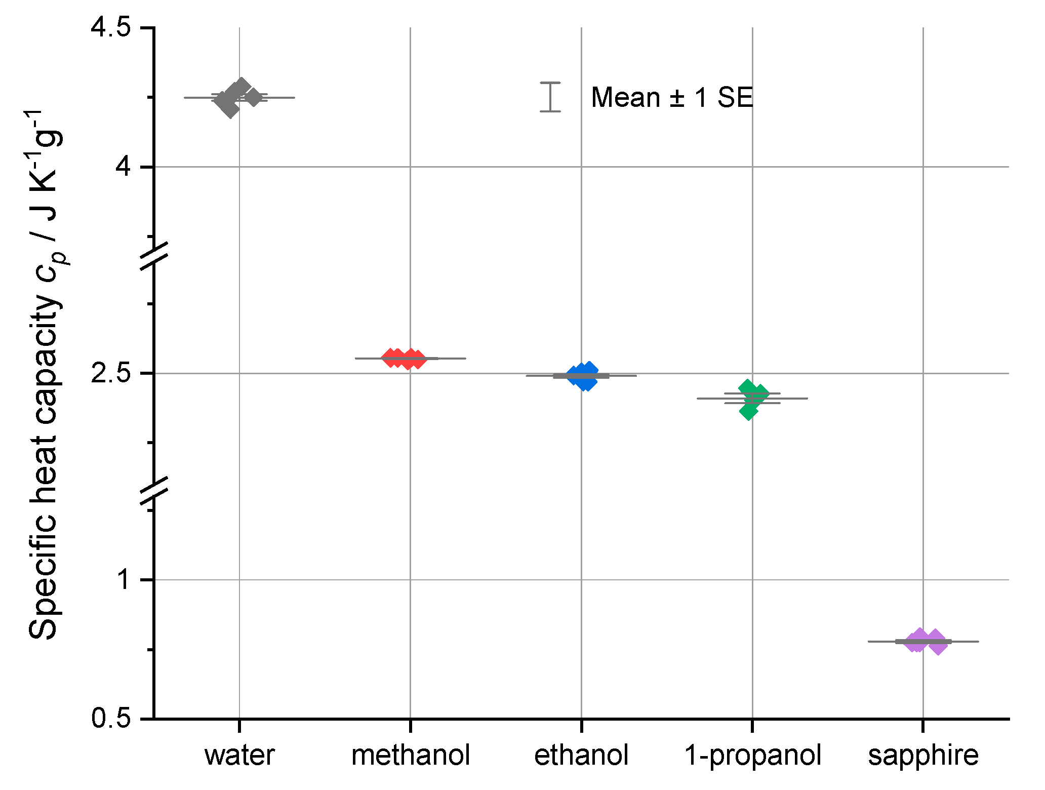
The raw heat flow data necessary to calculate the heat capacities of the samples measured by the Heat–Cool method for water, sapphire, methanol, ethanol, and propan-1-ol are presented in
Table 1a–e, as are the calculated specific heats.
From the earlier propagated uncertainty calculation value of δcp of ±0.012 J K−1 g−1, the standard deviation values for the cp values obtained by repeated measurements are significantly larger and suggest the values should only be reported to two decimal places.
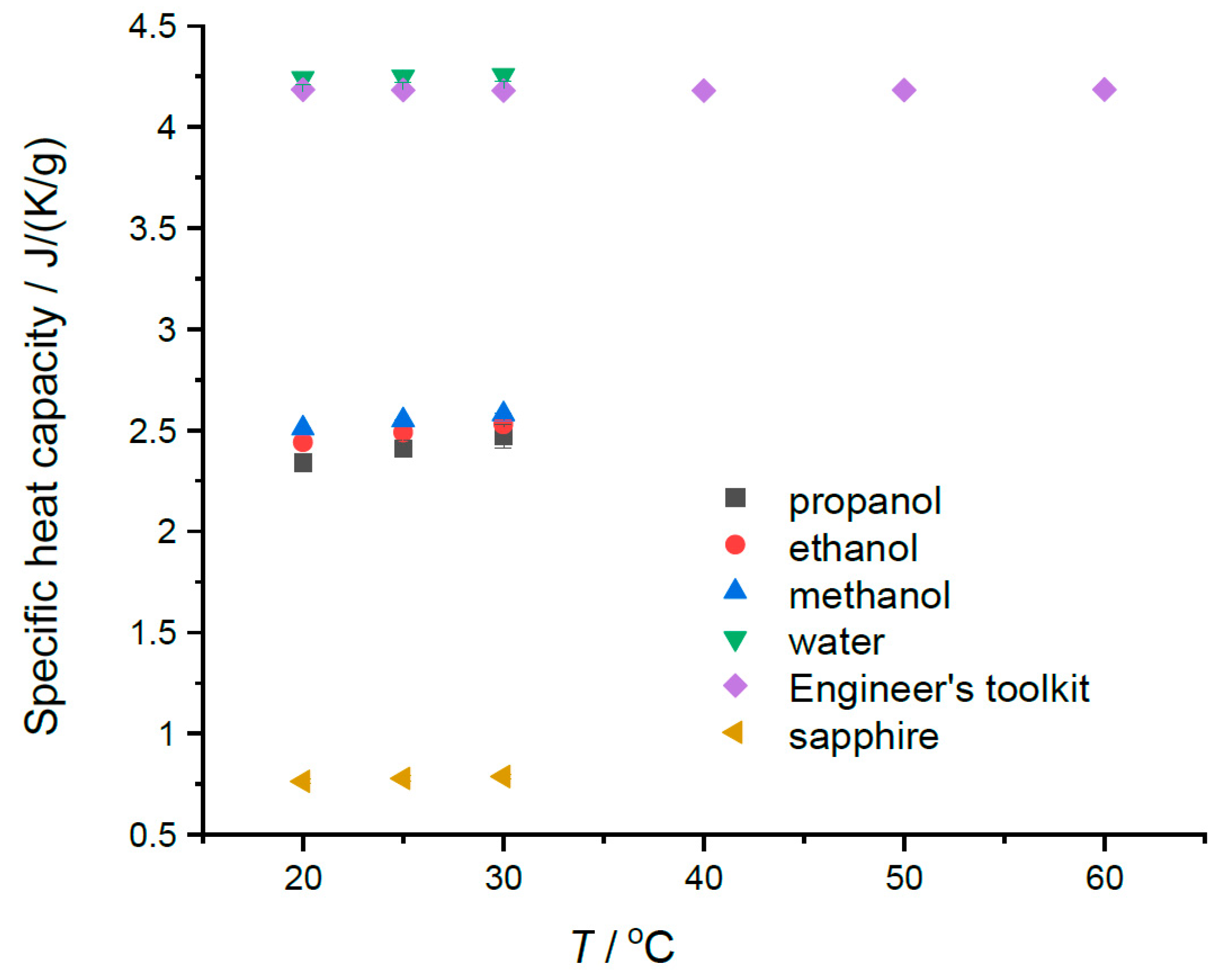
The modest temperature dependence of the specific heats in the region of 20 to 30 °C can be seen in
Table 1a–e and in
Figure 3. A weak but discernible temperature dependence is noted for the alcohols, as well the fact that the specific heats of alcohols are largest for the lowest mass alcohol, methanol. The opposite is true for molar heat capacity values. The specific heat of sapphire does show increasing values in this temperature range. Our water data seem to show very slight increasing values with temperature in this range; however, the uncertainties in the values (±0.03) suggest that the sensitivity of the instrument in this range is not great enough to detect the known decrease of 0.004 J K
−1 g
−1 for the specific heat capacity for water in the region of 20 to 40 °C.
Figure 3 indicates a minimum value between 30 and 40 °C. The relevant data are provided in
Table 1a. However, the alcohol results do suggest that the Heat–Cool method can, with care, measure the temperature dependences of liquid-specific heat capacities over modest temperature ranges.
5. Conclusions
The Heat–Cool method is presented as a simpler procedure to measure liquid heat capacities with DSC. The ease of use and agreement with the literature in the range of 1–2% are illustrated.
The major sources of uncertainty in the Heat–Cool method when measuring liquids seem to come from mass tolerances between the reference and sample pans, how samples are prepared in the DSC pan, and interferences in the DSC cell. The last one mainly entails minor oxidation inside the cell and can be managed easily enough through proper maintenance and periodic cleaning of the cell. However, how the pans are manufactured remains a noticeable source of uncertainty since current production tolerances are large enough to produce noticeable differences in the pan weights. Selecting matching pans by weight prior to sample preparation reduces this uncertainty. Sample preparation is a significant factor for controlling uncertainty in the experiment, which primarily entails maintaining a large ratio between the sample mass and the pan mass so that the majority of the measured heat flow signal is attributable to the sample. These uncertainties are not unique to the Heat–Cool method, but they become the largest contributors since the realized deviation from the literature values—hence, the uncertainty in estimating the Heat–Cool method—is significantly lower than other current methods.
When measuring the heat capacities of liquids, preparation is even more significant because of the potential for the heat of vaporization of the liquid contribution to the recorded heat flow. The amount of liquid added to the sample pan affects the volume of the headspace above the liquid, which significantly affects the vapor pressure and the amount of sample that can vaporize. As a result, it is important to use a large volume of liquid to reduce the headspace in the sample pan and reduce two phase effects.
Ultimately, the Heat–Cool method poses the opportunity to improve data quality and ease of use of DSC for measuring liquid and solid heat capacities. In addition to simply reducing uncertainty in heat capacity measurements, the Heat–Cool method is robust enough to allow for the collection of heat capacities, even of liquids, as functions of temperature, perhaps even above their boiling point. There is significant potential for the adoption of this method to improve how this key thermodynamic property is measured.


