Article

Assessment of Semi-Empirical Soot Modelling in Turbulent Buoyant Pool Fires from Various Fuels

Institut P’, Fluides-Thermique-Combustion, Centre National de la Recherche Scientifique, Ecole Nationale Supérieure de Mécanique et d’Aérotechnique, Université de Poitiers, 86961 Chasseneuil du Poitou, France
*
Author to whom correspondence should be addressed.
Thermo 2023, 3(3), 424-442; https://doi.org/10.3390/thermo3030026
Submission received: 23 May 2023 / Revised: 18 July 2023 / Accepted: 1 August 2023 / Published: 7 August 2023
(This article belongs to the Topic Heat Transfer Enhancement and Applications)

Abstract

:
The objective of this work is to assess the accuracy and limitations of two different semi-empirical soot models: the Laminar Smoke Point (LSP) and soot-yield approach. A global soot formation model based on the LSP concept is embedded within FDS6.7. Quantitative comparisons were made from turbulent buoyant pool fires between several computational results and well-instrumented experimental databases on the soot volume fraction, mass loss rate, heat release rate and gas temperature. The LSP model in combination with soot oxidation and surface growth is validated for most of the methane, ethylene and heptane turbulent buoyant pool fires, covering a wide range of fuel likely to form soot. This paper aims to broaden the scope of the validation of the available semi-empirical soot modelling. For the porous methane and ethylene burner, the LSP model was found to provide a better description of the soot volume fraction. The overall visual soot distribution is also numerically reproduced with the soot-yield approach, but as expected, there are some differences between the prediction and the measurement regarding the magnitude of soot volume fraction. The computed radiant heat flux was compared with experimental data for heptane flame, showing that predictions using both the LSP and soot-yield models were found to be twice the value of experimental data, although the measured HRR (Heat Release Rate) is reliably reproduced in the numerical simulation. For the heptane buoyant pool fires, a sufficient accuracy of the numerical model is confirmed only in some of the locations as compared to the experimental results. It is demonstrated that neither the temperature nor the soot volume fraction can be reliably calculated in the necking flame flapping region when the pyrolysis rate of condensed fuel (heptane) is coupled with radiation/convection heat feedback. This implies that an accuracy of prediction on the turbulent buoyant pool fires depends on the studied fire scenario regardless of the semi-empirical soot models.

1. Introduction

For a heavily sooting fire at hazardous scales of 1 m, the majority of the luminous thermal radiation in fire plume is derived from the visible part of the flame with a temperature above 500 °C. Sooting fire modelling is a challenging task because of the complexity of interactions between several processes and the large range of length and time scales involved. The fire spread over condensed fuel surface is significantly affected by soot due to great strength of flame radiation [1]. There is a large body of literature on soot formation in laminar flame for both liquid and gaseous fuels. Non-buoyant ethylene laminar jet diffusion flames have been modelled by assuming the nucleation and growth of soot are first-order functions of acetylene concentrations [2]. Anderson et al. [3] have shown that even a small quantity of aromatic hydrocarbons in the fuel can significantly increase soot emissions. Extensive efforts are devoted in CFD (Computational Fluid Dynamics) codes to the semi-empirical soot models, providing a good compromise between detailed chemistry and empirical models in terms of generality and computational cost. Leung et al. [4] in their study of laminar flame developed a soot growth rate based on the formation of two and three-ringed aromatic species from single-ring aromatic species using a simplified reaction mechanism. For reactive free buoyant plumes, various semi-empirical models involving the inception, coagulation, surface growth and oxidation processes rely partially on two pre-exponential factors and experimental calibrations [5]. Good progress has been achieved over the last decades in the soot modelling of turbulent flames. Research [6] on soot formation in turbulent kerosene/air jet diffusion flames suggests that the growth of aromatics is the rate-limiting step rather than the formation of the first ring. Soot production in fire plumes is a highly complex subject due to the spatially varying formation and oxidation processes, the influence of turbulent fluctuations as well as effects of temperature and nature of fuel. A global soot model (LSP) is combined with a probability density function in Large Eddy Simulation to account for unresolved subgrid-scale fluctuations of turbulent flames [7] by imposing a mass low rate of fuel. It is now well recognised that the main challenge in modelling the soot of heptane fires is to take into account the interaction of radiation and soot formation in the turbulent regime [8]. The consensus provided by previous studies [1,2,3,4,5,6,7,8] is that soot formation and oxidation models in combustion systems have a profound influence on the prediction of thermal radiation, which affects fire growth.
In this work, the global soot model [7], which is based on the classic principle of smoke point height to account for the fuels likely to produce soot in well or under-ventilated conditions, is implemented in FDS6.7 (Fire Dynamics Simulator) [9] in which an empirical model such as the soot-yield approach is used for specific combustion conditions as well-ventilated fires. It is worthwhile to note that most of the cases studied in the past [10,11] were made for two-dimensional, axisymmetric jet flames by using the acetylene/benzene based-soot model depending on detailed PAH (PolyAromatic Hydrocarbons) chemistry. However, it is difficult to perform the computations for three-dimensional turbulent fire with a coupling between the pyrolysis rate of condensed fuel, e.g., heptane, and radiation/convection heat feedback by using the acetylene/benzene based-soot model. Soot chemistry involved in large-scale fires for providing the local concentration of soot precursory species, such as acetylene (C2H2), benzene (C6H6), phenyl (C6H5) and OH•, is often complex and not totally numerically resolved by using an EDC (Eddy Dissipation Concept) combustion model [9]. Application in three-dimensional turbulent pool fires from a porous burner [10] and liquid fuel [11,12] are presented in the current work by using a Laminar Smoke Point (LSP) model. The advantage of the present soot model is that the LSP height of any practical fuel can be measured, although the exact elementary reactions of various flammable materials are generally unknown. This provides a general and practical solution for three-dimensional turbulent fire simulations in soot modelling with the best tradeoff between accuracy and cost. Numerical results show that the profiles of the temperature and soot have a relatively fair agreement with the available experimental data for a porous burner, but the results vary significantly with a liquid fire such as heptane. When the computed radiant heat flux was compared with experimental data for heptane flames, the predicted value is found to be twice the one of the measurements. The scope of the validation of FDS6.7 to model sooting fires at a large scale with the available semi-empirical soot modelling is broadened.

2. Numerical Modelling

The transient equations of mass, momentum, energy and species conservation are the basis of the hydrodynamic model. A detailed description of the three-dimensional physics-based model can be found in the FDS6 user guide [9]. This section provides mainly a comprehensive methodology to take into account the various thermo-physical phenomena involved in fire.

2.1. Combustion Model

Reactions from Westbrook [13] are used to estimate carbon monoxide production thanks to the two following sequential semi-global steps:
C m H n + m 2 + n 4 O 2 m C O + n 2 H 2 O
C O + 1 2 O 2 C O 2
We calculate the turbulent reaction rate with an extended Eddy Dissipation Concept (EDC) [9].
ω ˙ i = ρ d Y i d t = ρ ξ τ m i x ( Y i Y i 0 ) + ( 1 ξ ) d Y i d t
Here, ρ denotes the density, and Yi denotes the species mass fraction. At the start of a time step, each cell has an initial concentration, Y i 0 , of species such as reactants, products, and inerts that exist with some degree of mixing. For a diffusion flame, each cell is completely unmixed at the start of a time step. Once mixed, species can react based on specified kinetic parameters—reactions may be infinitely fast or governed by an Arrhenius rate law. Fast chemistry is used for the primitive fuel oxidation (cf. Equation (1)), and the mixed reactor known as the fine structure region is treated as a perfectly stirred reactor. At any point in time, the composition of the computational cell may be determined by combining the unmixed and mixed portions via the unmixed fraction, ξ , which is defined as the fraction of mass within the cell existing as either 0 or 1. We use a key mixing timescale, τ m i x , to relate approximately the three processes of diffusion, subgrid-scale advection, and buoyant acceleration [9]. In a Large Eddy Simulation, turbulence is modelled using a Deardorff’s approach via eddy viscosity to which the diffusion time is attached. The modified Arrhenius parameters from Andersen [14] are used to create a mixed reaction mechanism; in this way, fast chemistry is combined with a finite-rate reversible carbon monoxide reaction (2).

2.2. Soot Formation Model

In FDS6.7 [9], a simple soot conversion model is based on the fraction of fuel mass that is converted into soot within a thin flame zone. The soot formation rate, ω ˙ s , is derived from the fuel reaction rate via soot yield as:
ω ˙ S = d ρ Y S d t = y s o o t _ y i e l d W F W S ω ˙ F
Here, WF and Ws denote the fuel and soot molar weight, respectively. A soot-yield value, ysoot_yield, can be experimentally determined only in well-ventilated conditions, e.g., 0.037 for heptane and 0.043 for ethylene [15]. However, these values change significantly for under-ventilated fires, and they cannot be experimentally determined.
Physically, along the height of a laminar diffusion flame, three soot regions can be observed: soot inception, soot surface growth and soot oxidation with the respective source forms:
ω ˙ i = ω ˙ s , N + ω ˙ s , G + ω ˙ s , O
In the second approach, soot concentrations obey a reaction equation where soot formation rate is determined from Laminar Smoke Point (LSP) relations depending on the nature of the fuel [7].
ω ˙ s , N = A f ρ 2 T 2.25 f f s t 1 f s t exp ( 2000 / T )
Here, f represents the conserved Schvab–Zeldovich mixture fraction, which is involved in the soot inception process.
f = Y F + Y P 1 + s
Regarding Af, the pre-exponential factor, it is the only parameter which takes into account the propensity of the fuel to produce soot. For ethylene, Af has been initially set at 4.1 × 10⁻⁵ with an LSP height of 0.106 m in the laminar flame modelling [7]. According to Equation (8), which is its reverse proportionality relationship, Af for heptane is computed equal to 2.9 × 10⁻⁵ from an LSP height of 0.147 [16].
A f , F u e l A f , C 2 H 4 = L C 2 H 4 L F u e l
In the case of a multi-component mixture, the average pre-exponential factor of the mixture, Af,mix, can be calculated from the molar fraction of each individual component, Xi, as,
A f , m i x = A f , i × X i
Physically, there is no fundamental difference in the soot inception process between the various global approaches [17,18,19]. Thus, the soot surface growth term in Equation (5) taken from the work of Moss [18] is combined with the soot inception model of Delichatsios [19]. The surface growth rate [18] is usually evaluated as follows:
ω ˙ s , G = C γ ρ T 1 / 2 X F exp ( T γ / T ) N 1 / 3 ( ρ Y s ) 2 / 3
Here, T denotes the local temperature, N denotes the soot number density, and XF denotes the mole fraction of the parent hydrocarbon. The parameters C γ a n d T γ , in the heterogeneous processes of soot surface growth, are experimentally calibrated in a diffusion flame [18]. Regarding soot number density, N, more information is available for the soot particulate surface area per unit mass of soot As with a measured approximate value of 160 m2/g [7]. Equation (11) provides a mean diameter of the primary soot particulates dp.
d p = 6 ρ s A s
dp can be estimated roughly to be 0.02 μ m .
Soot number density per unit mass of mixture N is then evaluated from the soot mass fraction, Ys, by considering soot particulates as spherical:
N = 6 Y s π d p 3 ρ s
Contribution of the soot surface growth to its formation becomes quantitatively important only near the flame sheet in the high-temperature regions due to its higher activation temperature ( T γ = 1.26 × 10 4 K ) [18].
Although several species can be involved in soot oxidation during hydrocarbon diffusion flames, principally O2, O and OH radicals, the soot oxidation reactions collectively sum to:
Csoot + O2 → CO2
The temperature dependence of the soot oxidation rate [20] is expressed as follows:
ω ˙ s , O = 4.7 × 10 10 Y s Y o exp ( 211000 / R T )
Here, R denotes the gas universal constant. LES (Large Eddy Simulation) allows us to capture the strong fluctuations of the buoyancy-induced turbulent flow in terms of temperature and chemical species used in such a semi-empirical soot model.

2.3. Boundary Condition at Interface

Over the surface of the porous burner, the boundary condition at the burner exit plane is prescribed by the distribution of the total mass loss rate.
The evaporation rate of heptane above its liquid surface is governed by Stefan diffusion [21] as a function of the liquid temperature and the fuel vapor pressure.
m ˙ F = ρ D L Nu l n 1 Y F , 1 Y F , i .
In an equilibrium state, the mole fraction of the fuel vapor, YF,i, above the liquid surface is determined from the Clausius–Clapeyron relation. The liquid fuel itself is treated to be thermally thick; a one-dimensional heat conduction equation for liquid temperature is applied. The convective heat flux, q ˙ c o n v " , received at the liquid surface is calculated from near-wall law. In fires, the radiation loss term in the enthalpy equation is generally calculated by solving the Radiation Transfer Equation (RTE) with a ray-based method, such as the discrete ordinate method [9]. This allows us to compute the radiative heat flux, q ˙ r a d " , received at the liquid surface. Since soot is usually the most important combustion product controlling the thermal radiation, the gas behaves as a grey medium, and one absorption coefficient without spectral dependence is employed in RTE [9]. For modelling the evaporation of the liquid fuel as heptane, the thermal properties, absorption coefficient and heat of vaporisation used in the model are specified in Table 1.

3. Results and Discussion

The three-dimensional computational domain for the numerical simulation is shown in Figure 1. A successful fire modelling requires a numerical domain large enough to exclude the negative effect of boundary entrainment on flow field and cautious setup of boundary conditions. In all the calculations, we first test the size of the domain to avoid as much as possible the restriction on the flame spread while taking into account the main soot zone. On the surfaces of the open domain, a free boundary condition was prescribed, and zero gradient conditions are used for the far-field boundary values of the variables. Selected fire models have been verified and validated by Stroup and Lindeman [22]; they found that the large-scale eddies containing energy are fully described when the fire characteristic length spread over about sixteen computational cells. Such mesh size optimisation is meaningful only for the calculation of the fluid motion outside the flame zone. An extremely small grid size lower than 1 mm is required to fully resolve the characteristic flame thickness and complex buoyancy-induced turbulent flow instabilities, making practical fire simulations difficult. A series of grid sizes are tested according to this viewpoint [22], and the finally chosen grid size in an order of 0.5–1 cm usually gives grid-independent prediction for the most three-dimensional turbulent fire simulations, e.g., [23] with the best tradeoff between accuracy and cost. By using 16 processors through the parallel processing of a Linux cluster, the CPU time for a simulation with a physical time of about 30 s is approximately 48–72 h. It should be noted that a systematic deviation is not solely due to errors induced by the cell size. Rather, it is associated with uncertainties in other modelling aspects, such as the turbulent viscosity and combustion models [19].

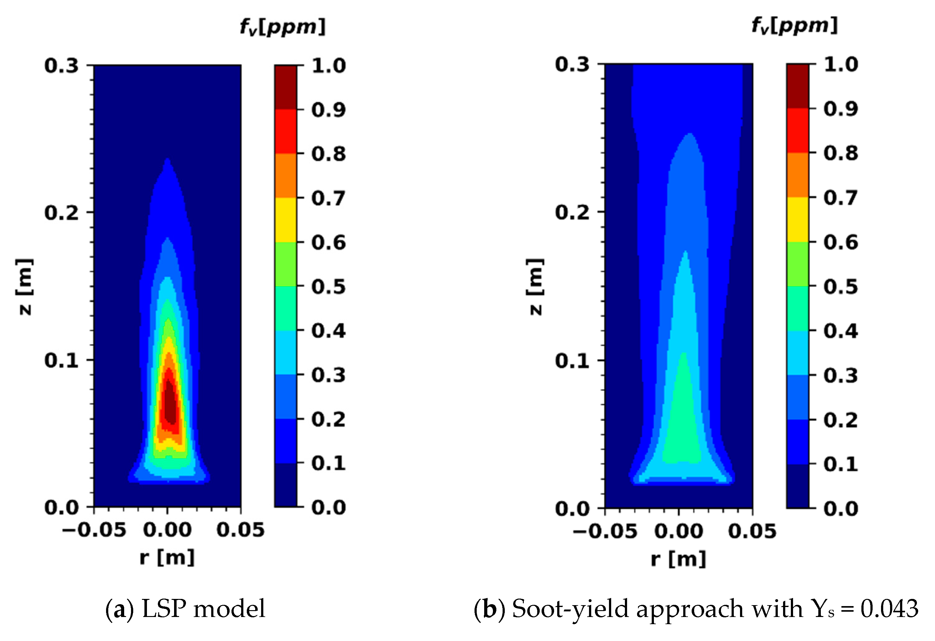
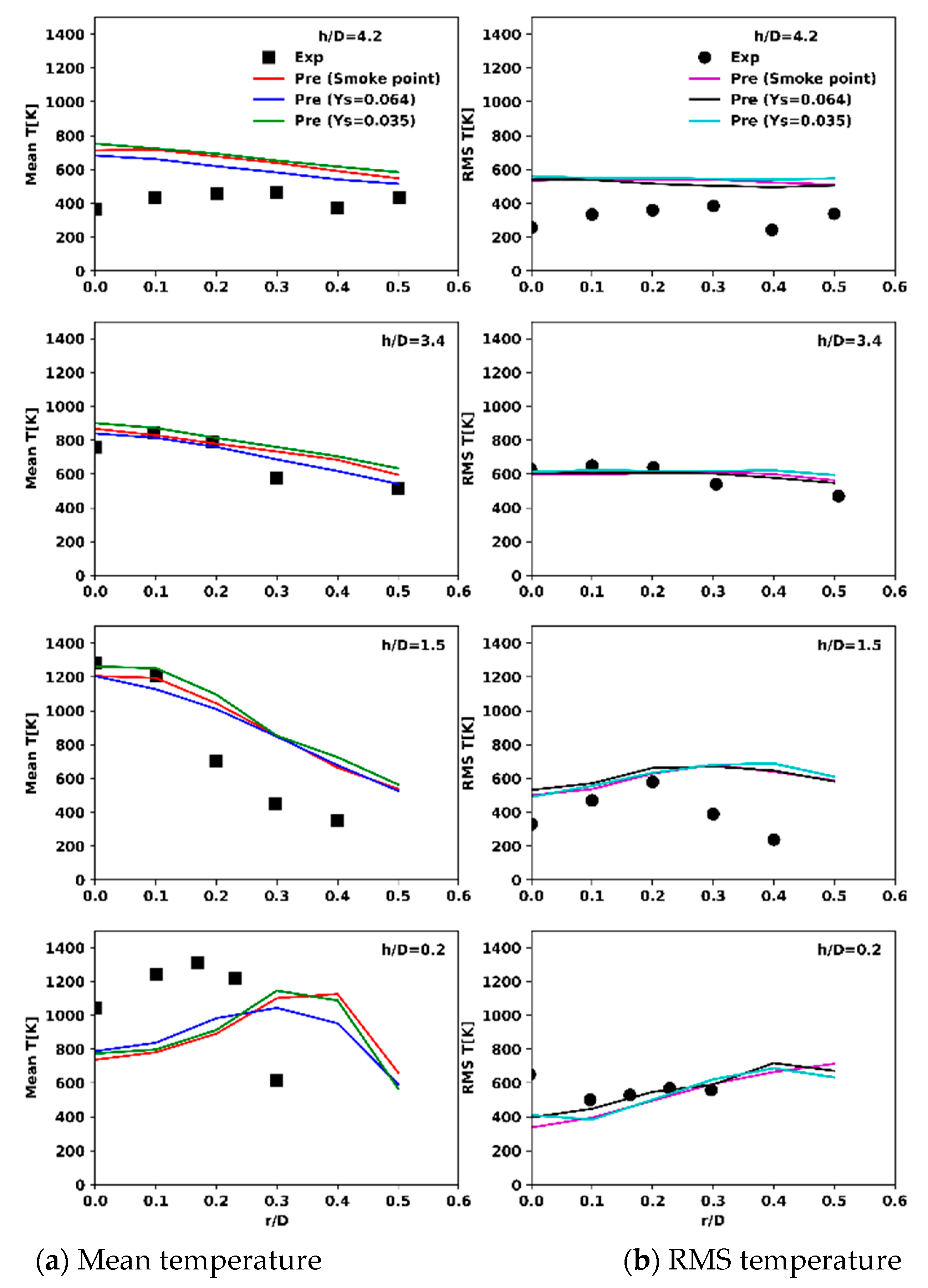
3.1. Methane and Ethylene Pool Fires

An application of the numerical code is first presented for a 7.1 cm porous burner [10] of weakly sooty methane and moderately sooty ethylene turbulent buoyant pool fires. The computational model of the circular burner is square with a 3.55 cm side in order to be equivalent with the burner area of reference [10]. The computational domain size of 1 × 1 × 0.6 m3 is chosen in width/length and height with a uniform grid size of 5 mm. The fuel flow rate is 0.0843 g/s for methane and 0.073 g/s for ethylene, which is prescribed at the fuel inlet; it corresponds to a 4.2 kW heat release rate. The experiments considered here were studied by Xin and Gore [10], in which soot volume fractions were measured by using the planar laser-induced incandescence (LII) technique. Average soot volume fractions were reported at different heights of 1D, 2D, 3D and 4D above the burner, where D is the diameter of the burner which is located at the centre of the bottom.
The temperature profile of a buoyant methane fire is presented in Figure 2a through the numerically computed temperature fields. The results shows a high magnitude of the gas temperature near the leading edge where the entrained air reacts with the fuel, involving a greater heat release above the flame base. The computed visible flame height, defined as the furthest axial location of the isotherm 500 °C [23], is around 0.38 m. The methane flame is considered as a non-smoking flame; however, the purity of the industrial methane gas is usually less than 93% with the composition of impurity as acetylene. By assuming that the 7% impurity contains heavy-sooting acetylene, the Af of industrial methane gas is given at 1 × 10⁻⁵ with Equation (10). Figure 2b shows contours of the calculated soot volume fraction with a peak value of 0.5 ppm. It seems that the purity of methane or its production of soot varies in a large range, and it can show a difference with pure methane gas. The maximum of the soot volume fraction is numerically reproduced in the flame core where we can observe gaseous mixtures that are relatively hot and rich in fuel. In the plume region above the flame, the soot volume fraction diminishes gradually. It can be related to the decrease in temperature of the gas and the dilution with cold air entrained by convection.
The comparison of predicted and measured soot profiles at different heights is shown in Figure 3. The soot volume fraction is measured by using the laser-induced incandescence technique (LII), which relies on the detection of the thermal radiation from the soot particles that have been heated up to the vaporisation temperature. The accuracy of such a measurement method depends on the accuracy of the proportionality constant required for correction due to attenuations of both the laser beam and the collected signal [10]. At 1D height (about 7.1 cm), the predicted symmetrical structure is not observed in the experimental soot distribution. This could be attributed in part to the spatial averaging of the experimental data turbulent wrinkled structures. Furthermore, at this position, an over-prediction of about 10% in the soot peak at the centre is observed, which does not affect the predicted soot volume fraction downstream. At 2D, the numerical soot volume fraction is significantly lower compared to the experimental one, and it shows a sharper peak in comparison with the experimental data. In fact, the EDC type is a temperature-independent combustion model, which lacks the ability to predict the transient phenomena of soot production at the location of 2D where the flame necking phenomenon may take place with the frequencies of flame presence/absence. Overall, the prediction of radial profiles at 3D and 4D far away from the fire source in a consistent or continuous region is in good agreement with the experimental data. This result demonstrates the validity of Equation (9), which could be used for any fuel with unknown chemistry as long as the composition of impurity can be estimated.
The computed temperature fields of ethylene pool fire are shown in Figure 4a,b with a visual similarity compared to the gross structure of the methane case. The average visible height of the flame is roughly 0.4 m, and the maximum flame temperature is 1400 K close to the leading edge. Figure 5a,b presents the numerical soot volume fraction profile for an ethylene diffusion flame comparing LSP (cf. Figure 5a) and soot-yield models (cf. Figure 5b). With the soot-yield approach, the maximum of the soot volume fraction is numerically reproduced at the burner exit plane where the fuel–air mixture is relatively cool and rich in fuel. Physically, the LSP model predicts well the overall distribution of the soot volume fraction since incomplete combustion products such as soot take place above the fuel-rich core where heat is released as the fuel reacts with the entrained air. Ethylene fire results in an increase in the soot formation as compared to the methane case, which is in agreement with the experimental findings.
Figure 6 shows a comparison of the predicted soot volume fraction with the measurement at different heights for the ethylene pool fire. The predicted trends with the LSP model are similar to the measured ones, and the predictions are only in qualitative agreement with the experimental data. An over-prediction of about 20% by the LSP model at 1D near the fire source is observed, which suggests that the model underestimates locally soot oxidation associated with air entrainment and product dilution or overestimates soot nucleation. The quantitative disagreement might be also due to neglect of the soot formation endothermicity in the combustion model. Soot volume fraction distribution is also globally in good agreement with experimental data with the soot-yield approach, but as expected, there are some differences between the prediction and the measurement in the magnitude of soot volume fraction. Such an ethylene-turbulent pool fire is also solved by FLUENT with an Alternative Conditional Source-term Estimation method [7] so as to handle the interaction between turbulent flow and soot chemistry. A similar trend between FLUENT and FDS is found for the prediction of soot volume fraction as compared to the measured ones. This demonstrates the limitation of the current global soot model in the different numerical tools for accurately predicting the soot production of turbulent fires.

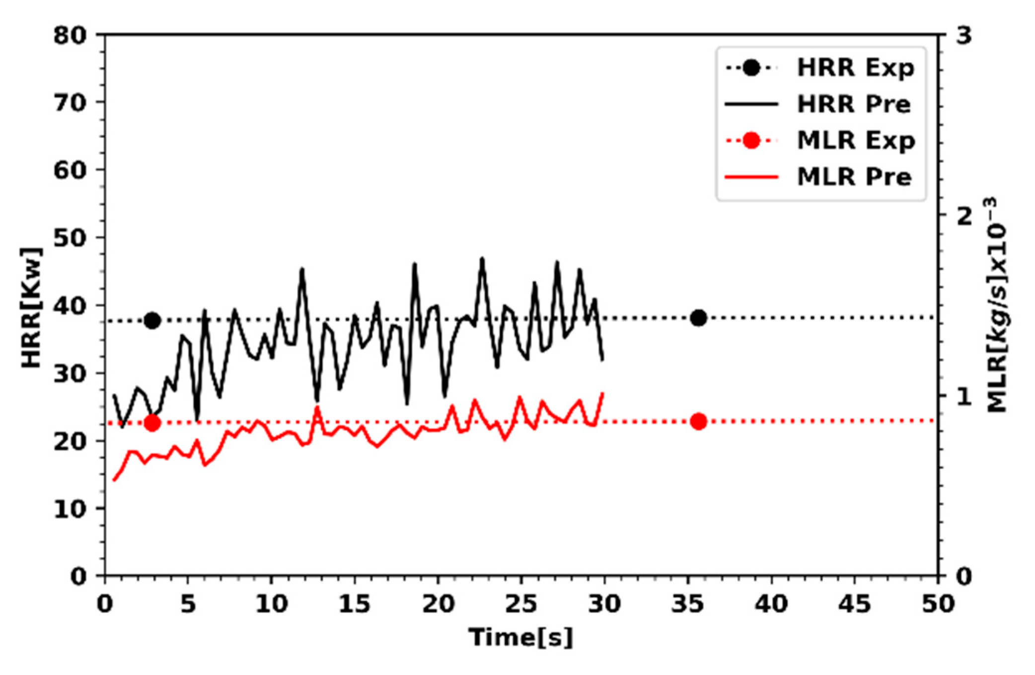
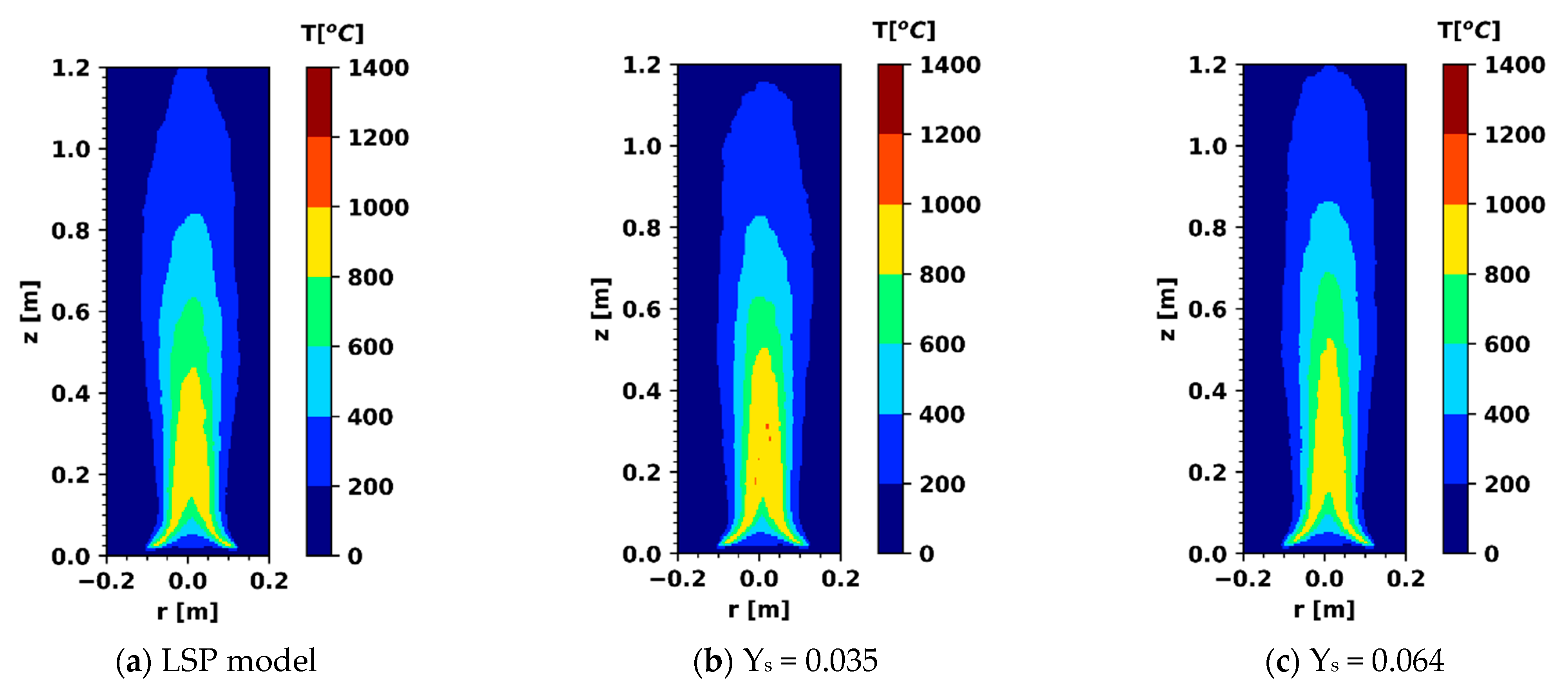
3.2. Heptane Pool Fire of 30 cm

Validation of the model was also performed against the heptane turbulent flames of 30 cm experimentally studied by Klassen [11]. In Figure 7, the red line illustrates the computed mass loss rate (MLR) of heptane fire from Stefan Equation (15), and the black line shows the calculated heat release rate (HRR) from the combustion model (cf. Equation (3)) in addition to the measured mean MLR and HRR. Sufficient volatiles are generated when the temperature of heptane reaches about 60 °C to sustain a burning flame. The heat released from the volatiles combustion is transferred back to the liquid fuel, and the liquid temperature continues to increase with time. The pyrolysis rate (cf. Figure 7) curve shows a growing trend with time, and it asymptotically reaches a peak of about 2 g/s when the liquid temperature approaches a steady state at the time of about 20 s. The computed MLR and HRR profiles with the LSP model are consistent with the measurement in terms of peak value with an under-prediction of about 20%.
The computed time-averaged temperature fields are shown in Figure 8a–c with a peak value of 1300 K occurring in the middle section of the fire and a lower temperature close to the pyrolysis surface. The predicted average visible height of the flame (T > 500 °C) from the LSP model is roughly 1.2 m, which compares well against experimental measurements of 1.31 m. By using the soot-yield approach, the predictions show an elongated flame length from 1 to 1.2 m with a reduction in soot-yield value from 0.064 to 0.035. This suggests that the temperature field is rather sensitive to the choice of soot-yield value.
Figure 9a–c present the calculated soot volume fraction for heptane diffusion flame comparing the LSP model (cf. Figure 9a) and soot-yield approach (cf. Figure 9b,c). We can note a significant difference between the LSP model and soot-yield approach regarding the peak values and general trends. With the soot-yield approach, the maximum soot is reproduced in the fuel-rich core, and the LSP model predicts maximum soot above the fuel-rich core where heat is released as the fuel reacts with the entrained air.
Figure 10a shows a comparison between numerically obtained soot profiles and experimentally measured soot data at four different heights above the pyrolysis surface. The experimental measurements indicate that at the bottom of the fire, few sooting regions are present, and the majority of soot formation takes place at the downstream locations of h/D = 1.5. The predicted peak from the LSP model is significantly higher than the experimentally estimated values at the location of h/D = 0.2, corresponding to a fuel-rich core known as the persistent zone where fuel is relatively cool and little oxygen has penetrated. This implies that at the location of h/D = 0.2 where the flame necking phenomenon takes place, the soot oxidation rate is underestimated with little oxygen at the bottom of the fire. This suggests that a more complex soot oxidation model including OH• radical should improve the result of the LSP model. Whereas, above the fuel surface at h/D = 0.2, the soot volume fraction is well predicted by using a soot-yield value of 0.035. The locations of h/D = 1.5 and 3.4 correspond to the intermittent region where the soot volume fraction is generally close to the measurements with the LSP model, suggesting the applicability of representing homogeneous soot chemistry status by mixture fraction. The location of h/D = 4.2 corresponds to a downstream thermal plume region where the rates of chemical reactions decrease exponentially as the temperature drops and more cold air is entrained. The higher soot volume fraction is mainly attributed to the radially convected soot particulate into the thermal plume due to a time-varying visible flame oscillation. The soot volume fraction downstream the flame tip at r/D = 4.2 is underpredicted by around 100% of the measurement, but far away from the centre, soot volume fraction predictions show similar trends as experimental measurements with deviations.
The computed profiles of RMS soot volume fractions, ( f v 2 ) , are compared with experimental estimations in Figure 10b. The prediction of RMS from LSP is in good agreement with the measurements only in the flame zone (h/D < 3.4). It should be noted that the prediction of RMS from any approach is significantly lower than experimental data in a downstream higher intermittent region at h/D = 4.2. In order to capture accurately the flapping behaviour of the reacting plume, improvements in subgrid soot variance modelling were made in a turbulent combustion model [8], and the comparison between the numerical and the experimental results is also not satisfactory. It seems that all the simplifying assumptions made in the soot model and uncertainties in soot measurements may induce a difference between them.
The time-averaged radial profiles of resolved temperature T and its RMS values, ( T 2 ) , at four heights of h/D = 0.2, 1.5, 3.4 and 4.2 where h is the height above the pyrolysis surface, are compared with experimental data in Figure 11a,b. Predicted temperature profiles from both LSP and soot-yield models are found to generally agree with the experimental data at h/D above 1.5. Whereas at the bottom of the fire, the temperature is either under-predicted at h/D = 0.2 or over-predicted at h/D = 1.5, indicating that LES is not able to accurately capture the necking flame flapping behaviour regardless of the soot model. The RMS component is generally in agreement with the experimental data, except at h/D = 1.5, where they are over-predicted for r/D > 0.2 by a factor of 100%. Since the LSP model relies strongly on temperature, its accurate prediction is imperative to improve soot prediction.

3.3. Heptane Fire of 23 cm

The heptane turbulent flames of 23 cm in diameter were experimentally studied by Garo et al. [12] and also used for validation of the model. Figure 12 illustrates the computed histories of MLR (Mass Loss Rate) and HRR (Heat Release Rate) for heptane pool fire in addition to the measured mean values determined from the evaporation rate of heptane. The pyrolysis rate curve shows a growing trend at the early stage during about 10 s, and it reaches a steady state with a mean value of 0.9 g/s, corresponding to a time-averaged HRR of about 38 kW. The perturbation of buoyancy-induced air flow entering the flame base results in an oscillating MLR with a variability of ±0.1 g/s. The computed pyrolysis rate and its associated HRR are consistent with the experimental data in terms of the time-averaged value.
The numerically computed temperature fields are described in Figure 13a–c. LSP and soot-yield models presents a slight difference regarding the temperature distribution. A low soot-yield value of 0.037 results in an elongated region of higher temperature (T > 900 °C), and inversely, a high soot value of 0.065 results in a decrease in the size of the region of higher temperature due to an enhanced radiation loss. The computed temperature field from the LSP model and the soot-yield value of 0.037 exhibit a similarity. The numerically computed temperature fields are compared with the experimental image as shown in Figure 14, which is only available in the half region (0 < r < 0.12 m). The temperature measurements in the compartment were performed with chromel–alumel thermocouples (type K) of a 0.5 mm wire with an uncertainty of 5–10% by taking into account a multitude of potential errors [23]. Although a similar gross structure of a buoyant fire is observed, an underestimation of about 200 °C is found at the flame base near the leading edge where the fuel and the oxidiser species come together in stoichiometric proportions and react exothermically, giving the maximum temperature. Numerical results exhibit a flame structure that is in agreement with experimental observations.
In order to make quantitative comparisons, Figure 15 shows the computed and the measured profiles of gas temperature along the height, z, at different radial locations (R = 0, 3, 6, 9, 10.5 cm). The computed temperature profiles from LSP and soot-yield models are almost identical in terms of location, shape and maximum value in comparison with the experimental data. There is a relatively good agreement between the prediction of axial profiles and the experimental data regarding the location of the flame sheet, which is characterised by the highest temperature. Near the leading edge at r = 9 and 10 cm, the predicted temperature peak is substantially lower than the experimentally estimated one. There is a substantial difference at r = 3 cm in terms of size of the region of higher temperature above 600 °C. The deviation in numerical gas temperature should be associated with uncertainties in subgrid diffusion as well as combustion models in laminar-like conditions near the leading edge above the flame base.
Figure 16a–c show the computed soot volume fraction (ppm) for the heptane diffusion flame of 23 cm with LSP and soot-yield models. As expected, an increase in soot-yield value from 0.037 to 0.064 results in a higher peak of soot volume fraction and a wider region of high soot volume fraction (>0.9 ppm). The region with the highest soot volume fraction from the LSP model is substantially larger than the estimated values from the soot-yield approach. In general, less soot formation with a soot yield of 0.037 results in an increase in gas temperature (cf. Figure 15).
Figure 17 shows the radiant heat flux over the liquid surface by using different soot models. Radiant heat flux over the fuel surface was measured by means of three Gardon-gauge-type radiometers with a solid angle of 150° for three radial positions of 0, 1/3R and 2/3R. The detailed measurement method can be found in Ref. [12]. As compared with the experimental data, an overestimation of the radiant heat flux by a factor of about two times over the liquid surface is mainly attributed to the predicted higher temperature in the fuel rich part of the flame (cf. Figure 15) regardless of the soot models. Globally, multiplying the soot-yield value by a factor of two, the radiant heat flux peak increases roughly by a factor of 30%. It is demonstrated that neither the temperature (cf. Figure 15) nor the soot volume fraction (cf. Figure 10) can be reliably calculated in the heptane fire simulations [8] even in a reduced scale. Since thermal radiation is a function of both gas temperature with T4 dependence and concentration of soot emitting species, a deviation in calculation of the radiant heat flux is associated with errors in the predicted temperature and soot fields.

4. Conclusions

A comprehensive model has been presented for soot formation in fires using the LSP concept and soot-yield approach. The methodology has been applied to predict soot volume fraction, and a sufficient accuracy of the LSP and soot-yield models is confirmed only for well-ventilated fires by imposing a mass loss rate of fuel. The present LSP model seems not capable of accurately predicting soot production and thermal field in highly oscillating heptane buoyant fires with a size in a range from 23 to 30 cm. A more meaningful and critical validation of the subgrid model would benefit the larger heptane flame. The soot-yield approach on the CFD code was also verified, and its application to turbulent pool fires can be achieved when its value is correctly selected.
Nonetheless, considering the uncertainties in measuring local soot concentration in heptane fires and the complexity of soot chemistry, these results demonstrate the potential of the present model for application in real fires. The soot inception temperature, the maximum temperature above which soot no longer forms, and the range of stoichiometry over which soot forms are all required model input parameters. At the base of non-premixed heptane flames, slight sooting cannot be captured by this model in its current form. In this region, soot formation is initially delayed and likely subject to surface area control; thus, the rate of formation of soot precursors must be taken into account. Near the flame sheet, the mechanism of HACA (Hydrogen Abstraction—Carbon Addition) is the dominant mode for the soot surface growth rate in the high-temperature regions dependent on the available surface area, but coagulation between PAH (PolyAromatic Hydrocarbons) and soot particles is quantitatively significant in the regions of low temperature. The soot oxidation rate is limited by the Arrhenius law for the decomposition of oxygen by the radical OH•. Considering the detailed and soot formation mechanisms are represented by the drastic simplifications and approximations made here, the presented numerical results are satisfactory and acceptable for larger fire simulations. It is worthwhile to note that as a consequence of enhanced radiation/convection heat feedback, turbulent or large-scale fires may produce the excess combustible gas from the pyrolysis of condensed fuel, e.g., heptane. A significant deviation of the numerical results in relation to experimental data can be found in the fuel-rich region for a turbulent or large-scale fire scenario in under-ventilated conditions. The discrepancy can be attributed to the omission of soot oxidation by the radical OH• due to the inadequate oxygen in the fuel-rich region where the detailed mechanisms of soot formation should be devoted.

Author Contributions

Conceptualization, H.-Y.W.; methodology, H.-Y.W.; software, H.-Y.W.; validation, L.A. and H.-Y.W.; formal analysis, B.C.; investigation, L.A.; resources, L.A.; data curation, L.A.; writing—original draft preparation, H.-Y.W.; writing—review and editing, B.C.; visualization, L.A.; supervision, H.-Y.W.; project administration, J.P.G.; funding acquisition, J.P.G. All authors have read and agreed to the published version of the manuscript.

Funding

This research received no external funding.

Data Availability Statement

The datasets generated during and/or analysed during the current study are available from the corresponding author on reasonable request.

Conflicts of Interest

The authors declare no conflict of interest.

References

  1. Guibaud, A.; Consalvi, J.L.; Orlac’h, J.M.; Citerne, O.J.M.; Legros, G. Soot production and radiative heat transfer in opposed flame spread over a polyethylene insulated wire in microgravity. Fire Technol. 2020, 56, 287–314. [Google Scholar] [CrossRef]
  2. Lui, F.; Guo, H.S.; Gregory, J.; Smallwood, J.; Ömer, L. Effects of gas and soot radiation on soot formation in a coflow laminar ethylene diffusion flame. J. Quant. Spectrosc. Radiat. Transf. 2002, 73, 409–421. [Google Scholar]
  3. Anderson, H.; McEnally, C.S.; Pfefferle, L.D. Experimental study of naphthalene formation pathways in non-premixed methane flames poped with alkylbenzenes. Proc. Combust. Inst. 2000, 28, 2577–2585. [Google Scholar] [CrossRef]
  4. Leung, K.M.; Lindstedt, R.P.; Jones, W.P. A simplified reaction mechanism for soot formation in nonpremixed flames. Combust. Flame 1991, 87, 289–305. [Google Scholar] [CrossRef]
  5. Nmira, F.; Consalvi, J.L.; Demarco, R.; Gay, L. Assessment of semi-empirical soot production models in C1-C3 axisymmetric laminar diffusion flames. Fire Saf. J. 2015, 73, 79–92. [Google Scholar] [CrossRef]
  6. Wen, Z.; Yun, S.; Thomson, M.J.; Lightstone, M.F. Modeling soot formation in turbulent kerosene/air jet diffusion flames. Combust. Flame 2003, 135, 323–340. [Google Scholar] [CrossRef]
  7. Yao, W.; Zhang, J.; Nadjai, A.; Beji, T.; Delichatsios, M.A. A global soot model developed for fires: Validation in laminar flames and application in turbulent pool fires. Fire Saf. J. 2011, 7, 371–387. [Google Scholar] [CrossRef]
  8. Chatterjee, P.; Wang, Y.; Meredith, K.V.; Porofeev, S.B. Application of a subgrid soot-radiation model in the numerical simulation of a heptane pool fire. Proc. Combust. Inst. 2015, 35, 2573–2580. [Google Scholar] [CrossRef]
  9. McGrattan, K.; Hostikka, S.; McDermott, R.; Floyd, J.; Weinschenk, C.; Overholt, K. Fire Dynamics Simulator, Technical Reference Guide, 6th ed.; National Institute of Standards and Technology: Gaithersburg, MD, USA, 2018. [Google Scholar]
  10. Xin, Y.; Gore, J.P. GORE, Two-dimensional soot distributions in buoyant turbulent fires. Proc. Combust. Inst. 2005, 30, 719–726. [Google Scholar] [CrossRef]
  11. Klassen, M.; Gore, J.P. Structure and Radiation Properties of Pool Fires; Technical Report NIST-GCR-94-651; US Department of Commerce: Washington, DC, USA, 1994. [Google Scholar]
  12. Garo, J.P.; Vantelon, J.P.; Lemonnier, D. Effect on radiant heat transfer at the surface of a pool fire interacting with a water mist. J. Heat Transf. 2010, 132, 023503. [Google Scholar] [CrossRef]
  13. Westbrook, C.K.; Dryer, F.L. Simplified reaction mechanisms for the oxidation of hydrocarbon fuels in flames. Combust. Sci. Technol. 1981, 27, 31–43. [Google Scholar] [CrossRef]
  14. Andersen, J.; Rasmussen, C.L.; Giselsson, T.; Glarborg, P. Global combustion mechanisms for use in CFD modelling under oxy-fuel conditions. Energy Fuels 2009, 23, 1379–1389. [Google Scholar] [CrossRef]
  15. Hurley, M.J.; Gottuk, D.T.; Hall, J.R., Jr.; Harada, K.; Kuligowski, E.D.; Puchovsky, M.; Torero, J.L.; Watts, J.M., Jr.; Wieczorek, C.J. SFPE Handbook of Fire Protection Engineering; Springer: Berlin/Heidelberg, Germany, 2015. [Google Scholar]
  16. Hunt, R.A. Relation of smoke point to molecular structure. Ind. Eng. Chem. 1953, 45, 602–606. [Google Scholar] [CrossRef]
  17. Frenklach, M.; Wang, H. Detailed modelling of soot particle nucleation and growth. Proc. Combust. Inst. 1990, 23, 1559–1566. [Google Scholar] [CrossRef]
  18. Moss, J.B.; Stewart, C.D.; Young, K.J. Modelling soot formation and burnout in a high temperature laminar diffusion flame burning under oxygen-enriched conditions. Combust. Flame 1995, 101, 491–500. [Google Scholar] [CrossRef]
  19. Delichatsios, M.A. A phenomenological model for smoke point and soot formation in laminar flames. Combust. Sci. Technol. 1994, 100, 283–298. [Google Scholar] [CrossRef]
  20. Lee, K.B.; Thring, M.W.; Beer, J.M. On the rate of combustion of soot in a laminar soot flame. Combust. Flame 1962, 6, 137–145. [Google Scholar] [CrossRef]
  21. Murty Kanury, A. Introduction to Combustion Phenomena; Gordon: New York, NY, USA, 1984; ISBN 0-677-02690-0. [Google Scholar]
  22. Stroup, D.; Lindeman, A. Verification and Validation of Selected Fire Models for Nuclear Power Plant Applications; NUREG-1824, Supplement 1; United States Nuclear Regulatory Commission: Washington, DC, USA, 2013; pp. 37–48. [Google Scholar]
  23. Acherar, L.; Wang, H.Y.; Garo, J.P.; Coudour, B. Impact of air intake position on fire dynamics in mechanically ventilated compartment. Fire Saf. J. 2020, 118, 103210. [Google Scholar] [CrossRef]
Figure 1. Computational domain and coordinate system for the numerical simulation.
Thermo 03 00026 g001
Figure 2. Computed fields of typical temperature (°C) and soot volume fraction above methane burner.
Thermo 03 00026 g002
Figure 3. Comparison between the predicted and measured [10] radial soot volume fraction profiles at 4 different heights for methane burner.
Thermo 03 00026 g003
Figure 4. Computed fields of the typical temperature (°C) above ethylene burner.
Thermo 03 00026 g004
Figure 5. Computed fields of soot volume fraction above ethylene burner.
Thermo 03 00026 g005
Figure 6. Comparison between the predicted and measured [10] radial profiles of soot volume fraction at 4 different heights of 1D, 2D, 3D and 4D above the burner, where D is the diameter of the burner.
Thermo 03 00026 g006
Figure 7. Computed pyrolysis rate and heat release rate for heptane pool fire.
Thermo 03 00026 g007
Figure 8. Computed time-averaged temperature fields with different soot models for heptane pool fire.
Thermo 03 00026 g008
Figure 9. Computed fields of soot volume fraction above heptane pool fire of 30 cm for the different soot models.
Thermo 03 00026 g009
Figure 10. Comparison between the predicted and measured radial soot volume fraction profiles and its RMS component at 4 different heights.
Thermo 03 00026 g010
Figure 11. Comparison between prediction and experiment for the radial distribution of mean temperature and its RMS component at 4 different heights.
Thermo 03 00026 g011
Figure 12. Comparison between the computed and measured MLR and HRR.
Thermo 03 00026 g012
Figure 13. Predicted temperature (°C) fields above heptane pool fire of 23 cm for the different soot models.
Thermo 03 00026 g013
Figure 14. Experimental temperature (°C) field above heptane pool fire of 23 cm.
Thermo 03 00026 g014
Figure 15. Comparison between the numerical and experimental profiles of gas temperature along the axis of the heptane pool fire at five radial positions.
Thermo 03 00026 g015
Figure 16. Predicted fields of soot volume fraction above heptane pool fire of 23 cm by using different soot models.
Thermo 03 00026 g016
Figure 17. Computed and measured radiant heat flux over the heptane surface.
Thermo 03 00026 g017
Table 1. Thermo-physical and combustion properties of heptane.
PropertyHeptane
Conductivity, k (W/m.K)0.17
Density, ρ (kg/m3)684
Heat capacity, Cp (kJ/kg.K)2.24
Pyrolysis heat, Lv (kJ/kg)321
Heat   of   combustion ,   Δ H c (kJ/kg)44,500
Boiling temperature, Tb (°C)98
Absorption coefficient (m−1)40
Disclaimer/Publisher’s Note: The statements, opinions and data contained in all publications are solely those of the individual author(s) and contributor(s) and not of MDPI and/or the editor(s). MDPI and/or the editor(s) disclaim responsibility for any injury to people or property resulting from any ideas, methods, instructions or products referred to in the content.

