
Traditional Yerba Mate Agroforestry Systems in Araucaria Forest in Southern Brazil Improve the Provisioning of Soil Ecosystem Services

Abstract
:1. Introduction
2. Material and Methods
2.1. Study Area and Sampling
2.2. Analysis of Soil ES Indicators
2.3. Analysis of Soil Attributes
2.4. Statistical Analysis
2.5. Analysis of Ecosystem Services Indicators of Soils
3. Results and Discussion
3.1. Soil Quality Variables in the Production Systems
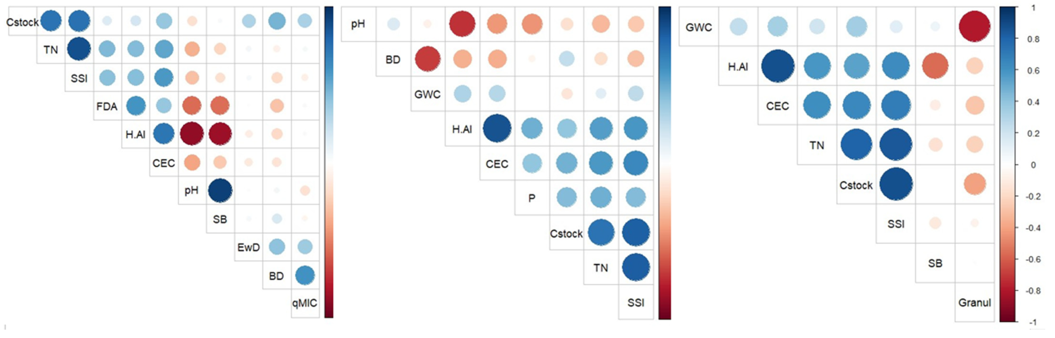
3.2. Correlations among Attributes
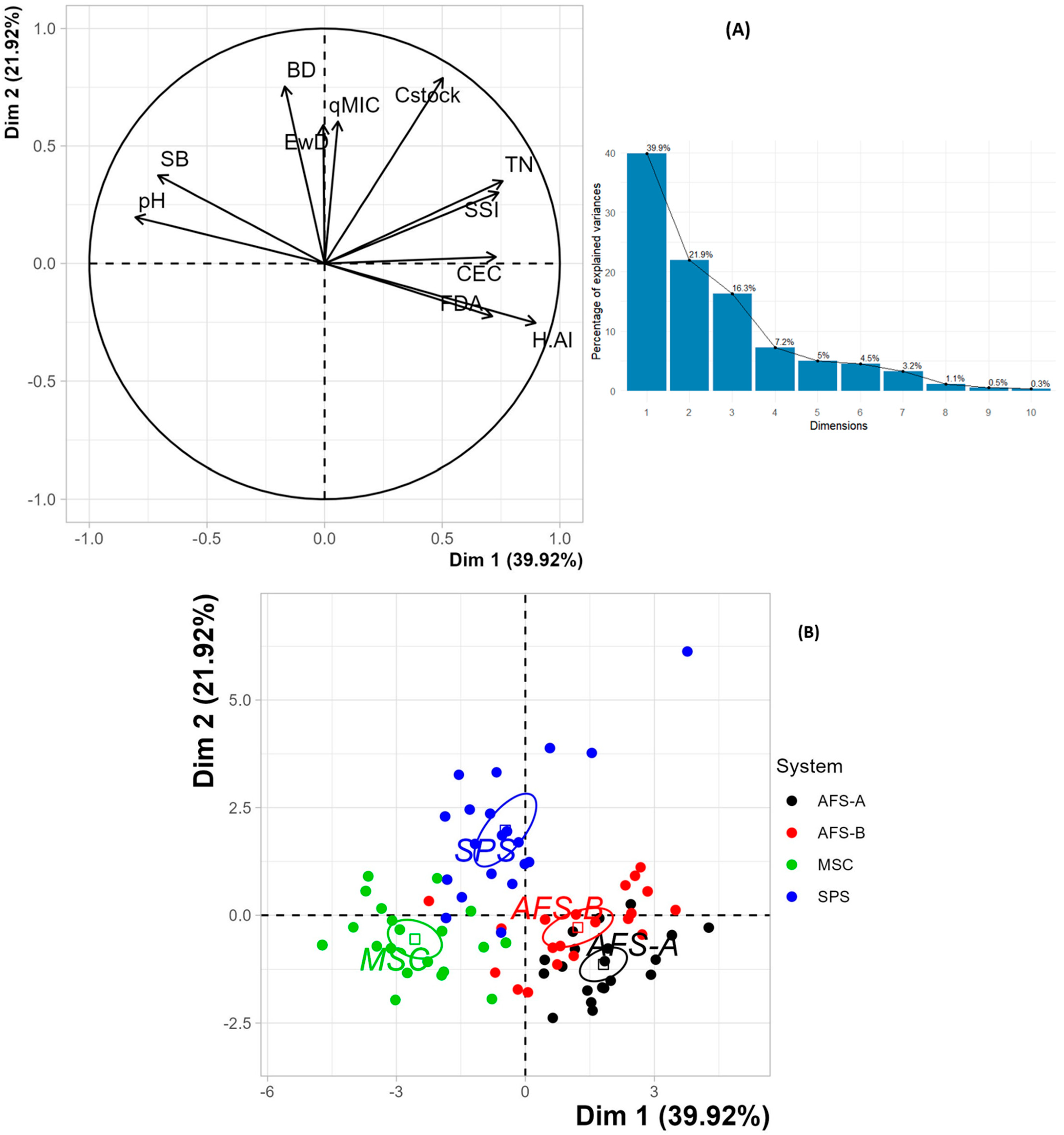
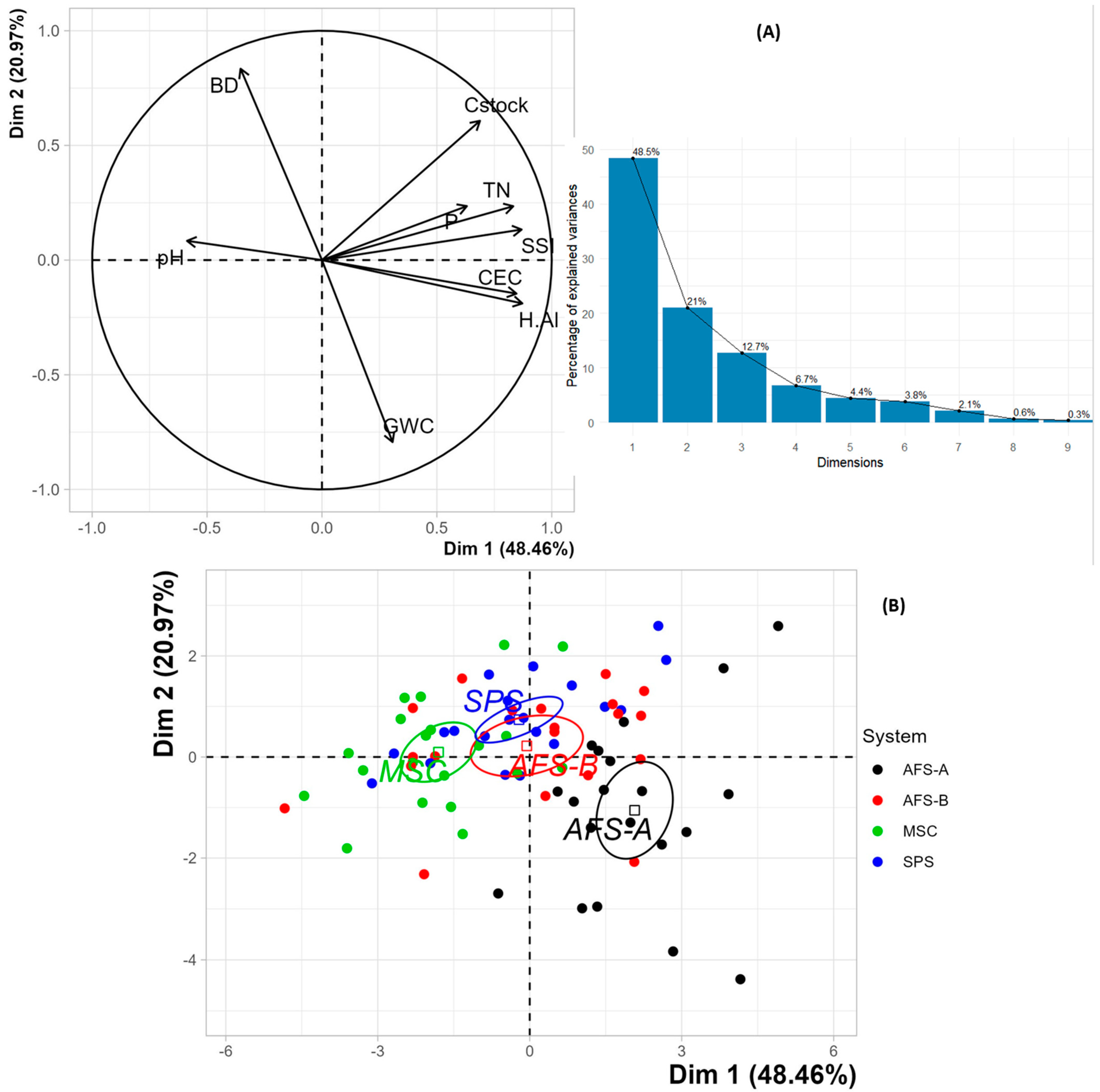
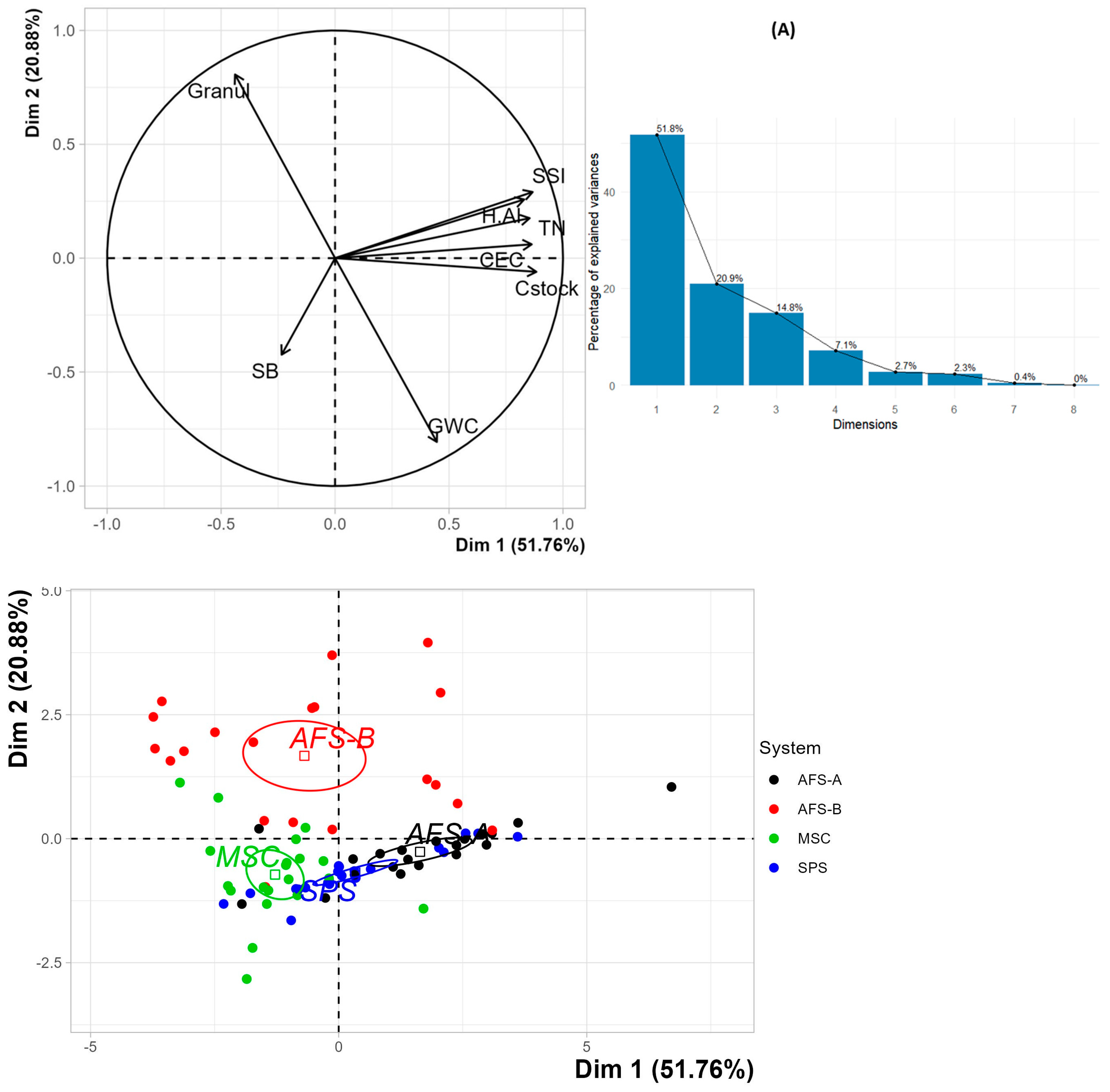
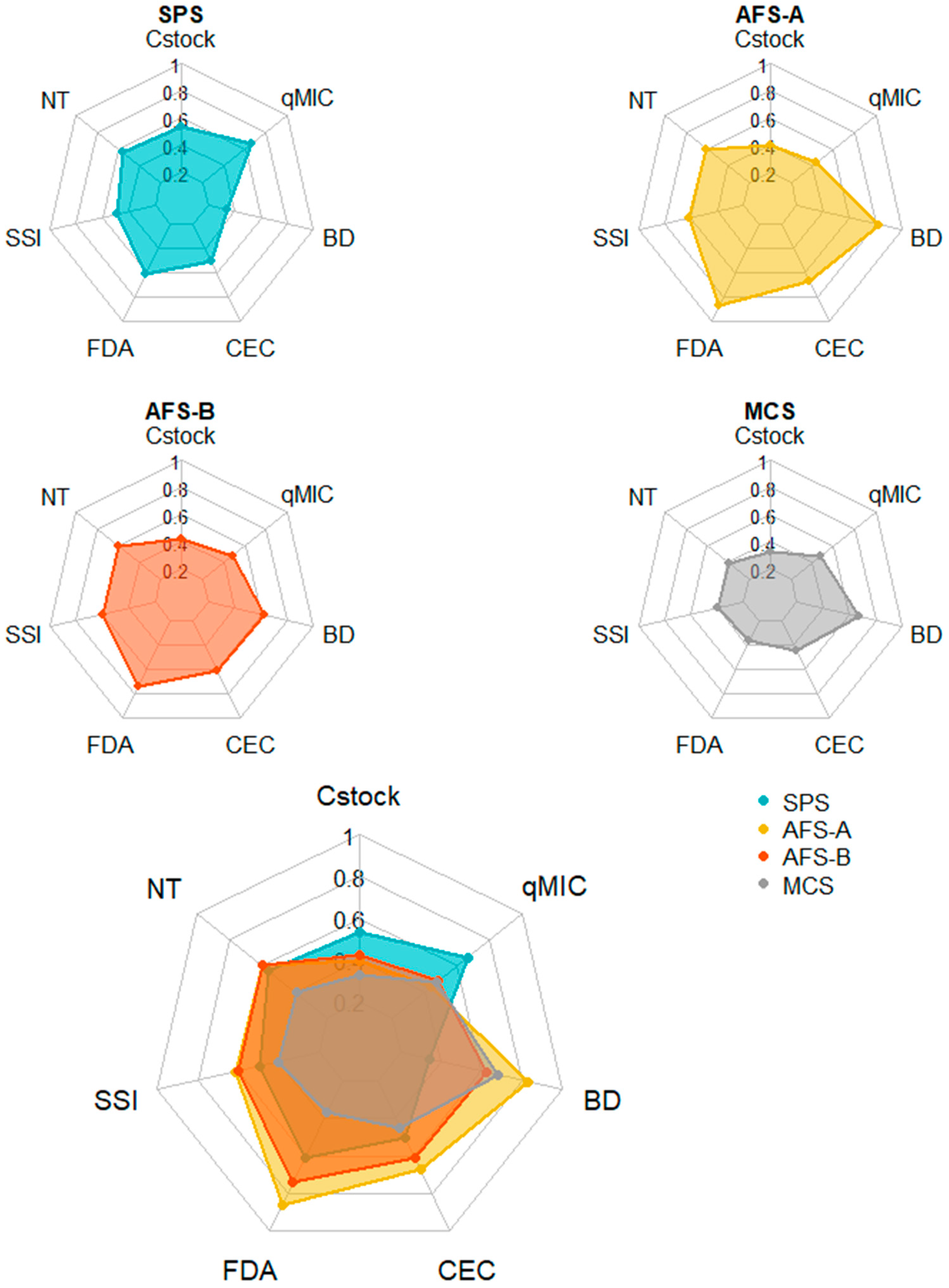
3.3. Soil Quality Indicators and Soil Ecosystem Services
4. Conclusions
Author Contributions
Funding
Data Availability Statement
Acknowledgments
Conflicts of Interest
Appendix A

| System | Layer | Statistics | pH | Al | H+Al | Ca | Mg | K | SB | CEC | TN | TC | P | Cstock | Sand | Silt | Clay | SSI | GWC | BD |
|---|---|---|---|---|---|---|---|---|---|---|---|---|---|---|---|---|---|---|---|---|
| SPS | 0–10 cm | Mean | 4.3 | 1.4 | 11.4 | 4.8 | 1.2 | 0.2 | 6.2 | 18.8 | 0.42 | 46.84 | 2.4 | 51.4 | 36.6 | 297.1 | 666.4 | 8.4 | 0.3 | 1.1 |
| S | 0.3 | 1.1 | 2.7 | 2.4 | 0.9 | 0.0 | 3.0 | 3.6 | 0.09 | 13.12 | 0.8 | 14.3 | 5.6 | 41.0 | 42.5 | 2.3 | 0.0 | 0.1 | ||
| CV (%) | 6.8 | 76.1 | 23.8 | 49.2 | 70.5 | 24.4 | 48.6 | 19.1 | 21.49 | 28.0 | 34.5 | 27.7 | 15.2 | 13.8 | 6.4 | 27.9 | 6.3 | 5.5 | ||
| 10–20 cm | Mean | 3.9 | 3.5 | 14.8 | 1.0 | 0.3 | 0.1 | 1.5 | 18.9 | 0.30 | 32.67 | 1.2 | 33.9 | 36.5 | 277.9 | 685.6 | 5.8 | 0.3 | 1.0 | |
| S | 0.1 | 0.9 | 2.7 | 0.9 | 0.2 | 0.0 | 1.1 | 3.2 | 0.06 | 7.56 | 0.5 | 7.5 | 15.1 | 49.2 | 50.6 | 1.4 | 0.1 | 0.1 | ||
| CV (%) | 2.4 | 24.8 | 18.3 | 85.3 | 69.3 | 24.7 | 73.4 | 17.1 | 19.51 | 23.1 | 42.6 | 22.0 | 41.3 | 17.7 | 7.4 | 23.6 | 19.4 | 6.1 | ||
| 20–40 cm | Mean | 4.0 | 3.8 | 13.7 | 0.5 | 0.1 | 0.1 | 0.7 | 17.6 | 0.24 | 27.39 | 0.7 | 58.5 | 29.0 | 252.6 | 718.4 | 4.9 | 0.4 | 1.1 | |
| S | 0.2 | 0.7 | 1.9 | 0.7 | 0.1 | 0.0 | 0.8 | 3.9 | 0.05 | 6.37 | 0.2 | 14.6 | 3.1 | 44.1 | 43.1 | 1.1 | 0.0 | 0.0 | ||
| CV (%) | 6.1 | 19.1 | 14.2 | 130.2 | 103.5 | 27.8 | 111.6 | 22.1 | 20.14 | 23.3 | 35.1 | 25.0 | 10.7 | 17.4 | 6.0 | 23.1 | 8.6 | 3.6 | ||
| AFS-A | 0–10 cm | Mean | 3.7 | 5.0 | 19.2 | 0.6 | 0.5 | 0.2 | 1.3 | 18.0 | 0.44 | 52.17 | 2.1 | 41.3 | 64.5 | 305.5 | 630.0 | 9.6 | 0.4 | 0.8 |
| S | 0.2 | 1.0 | 3.9 | 0.6 | 0.3 | 0.0 | 0.9 | 1.6 | 0.06 | 7.50 | 0.5 | 6.9 | 22.4 | 23.9 | 20.9 | 1.4 | 0.1 | 0.1 | ||
| CV (%) | 4.4 | 18.9 | 20.6 | 100.1 | 65.7 | 24.0 | 70.2 | 9.1 | 13.47 | 14.4 | 25.0 | 16.7 | 34.7 | 7.8 | 3.3 | 14.8 | 22.8 | 10.1 | ||
| 10–20 cm | Mean | 3.8 | 5.4 | 19.5 | 0.3 | 0.3 | 0.1 | 0.7 | 16.9 | 0.33 | 41.25 | 1.2 | 35.7 | 64.3 | 292.7 | 643.0 | 7.6 | 0.5 | 0.9 | |
| S | 0.1 | 0.8 | 3.0 | 0.3 | 0.2 | 0.0 | 0.4 | 2.6 | 0.05 | 6.03 | 0.5 | 7.8 | 22.8 | 22.1 | 18.2 | 1.1 | 0.2 | 0.1 | ||
| CV (%) | 2.6 | 14.5 | 15.3 | 76.3 | 79.2 | 19.4 | 60.9 | 15.6 | 16.28 | 14.6 | 43.7 | 21.9 | 35.5 | 7.6 | 2.8 | 14.3 | 31.1 | 11.4 | ||
| 20–40 cm | Mean | 3.9 | 4.8 | 17.6 | 0.2 | 0.1 | 0.1 | 0.4 | 21.1 | 0.25 | 31.48 | 0.5 | 61.8 | 58.2 | 271.6 | 670.2 | 5.7 | 0.5 | 1.0 | |
| S | 0.1 | 0.6 | 2.8 | 0.1 | 0.1 | 0.0 | 0.2 | 2.8 | 0.06 | 6.08 | 0.3 | 11.5 | 39.9 | 20.4 | 43.8 | 1.0 | 0.0 | 0.1 | ||
| CV (%) | 2.3 | 12.6 | 16.1 | 52.7 | 92.9 | 70.9 | 45.7 | 13.4 | 24.65 | 19.3 | 55.2 | 18.7 | 68.5 | 7.5 | 6.5 | 18.1 | 7.6 | 6.8 | ||
| AFS-B | 0–10 cm | Mean | 3.8 | 3.7 | 17.6 | 1.0 | 0.6 | 0.2 | 1.8 | 15.3 | 0.44 | 46.54 | 2.2 | 43.0 | 149.7 | 350.3 | 500.0 | 9.4 | 0.4 | 0.9 |
| S | 0.3 | 1.5 | 4.1 | 1.3 | 0.4 | 0.1 | 1.6 | 5.0 | 0.08 | 8.54 | 0.7 | 8.9 | 46.9 | 18.0 | 54.1 | 1.7 | 0.1 | 0.1 | ||
| CV (%) | 8.1 | 40.2 | 23.2 | 130.9 | 66.3 | 62.1 | 89.9 | 32.9 | 17.60 | 18.4 | 30.1 | 20.7 | 31.4 | 5.1 | 10.8 | 17.8 | 16.3 | 9.6 | ||
| 10–20 cm | Mean | 3.9 | 3.7 | 15.1 | 0.4 | 0.2 | 0.1 | 0.7 | 14.0 | 0.30 | 31.66 | 1.0 | 31.5 | 151.2 | 354.0 | 494.8 | 6.4 | 0.4 | 1.0 | |
| S | 0.3 | 1.5 | 5.0 | 0.3 | 0.1 | 0.0 | 0.4 | 3.1 | 0.05 | 5.75 | 0.3 | 6.8 | 52.1 | 20.4 | 69.0 | 1.0 | 0.1 | 0.1 | ||
| CV (%) | 7.8 | 40.9 | 33.2 | 92.4 | 63.8 | 33.0 | 60.3 | 21.8 | 17.13 | 18.2 | 32.8 | 21.7 | 34.4 | 5.7 | 13.9 | 16.2 | 18.8 | 8.2 | ||
| 20–40 cm | Mean | 4.0 | 3.3 | 13.5 | 0.3 | 0.2 | 0.1 | 0.5 | 16.8 | 0.24 | 25.44 | 0.7 | 50.7 | 153.8 | 345.8 | 500.4 | 5.2 | 0.4 | 1.0 | |
| S | 0.2 | 1.4 | 4.5 | 0.2 | 0.1 | 0.0 | 0.2 | 3.2 | 0.05 | 5.39 | 0.7 | 10.5 | 56.4 | 26.1 | 73.3 | 1.0 | 0.1 | 0.0 | ||
| CV (%) | 4.2 | 43.7 | 33.1 | 72.0 | 69.5 | 33.6 | 48.9 | 19.3 | 20.36 | 21.2 | 88.4 | 20.8 | 36.7 | 7.5 | 14.7 | 19.8 | 21.0 | 2.1 | ||
| MSC | 0–10 cm | Mean | 4.8 | 0.8 | 8.1 | 5.5 | 2.8 | 0.2 | 8.5 | 14.5 | 0.33 | 39.71 | 1.4 | 35.2 | 70.7 | 351.3 | 578.0 | 7.4 | 0.4 | 0.9 |
| S | 0.7 | 1.1 | 4.6 | 3.6 | 2.8 | 0.1 | 4.9 | 2.4 | 0.06 | 5.99 | 0.7 | 5.0 | 27.0 | 49.9 | 73.8 | 1.3 | 0.2 | 0.1 | ||
| CV (%) | 15.3 | 145.7 | 56.5 | 66.2 | 100.3 | 40.8 | 58.2 | 16.8 | 17.91 | 15.1 | 45.9 | 14.2 | 38.2 | 14.2 | 12.8 | 17.4 | 45.5 | 10.1 | ||
| 10–20 cm | Mean | 4.3 | 1.7 | 10.0 | 3.4 | 1.0 | 0.1 | 4.5 | 13.8 | 0.25 | 29.98 | 0.7 | 30.2 | 82.6 | 323.2 | 594.2 | 5.6 | 0.4 | 1.0 | |
| S | 0.5 | 1.4 | 4.4 | 3.2 | 1.0 | 0.0 | 3.9 | 3.8 | 0.04 | 5.20 | 0.4 | 6.4 | 39.3 | 36.5 | 62.7 | 0.9 | 0.1 | 0.1 | ||
| CV (%) | 12.6 | 82.0 | 44.2 | 94.2 | 95.1 | 26.1 | 86.4 | 27.8 | 16.87 | 17.3 | 47.5 | 21.3 | 47.5 | 11.3 | 10.5 | 15.9 | 16.0 | 7.8 | ||
| 20–40 cm | Mean | 4.3 | 2.0 | 10.4 | 2.1 | 0.6 | 0.1 | 2.8 | 12.2 | 0.20 | 23.24 | 0.5 | 52.7 | 76.6 | 294.0 | 629.4 | 4.3 | 0.4 | 1.1 | |
| S | 0.4 | 1.1 | 2.6 | 2.4 | 0.8 | 0.0 | 3.0 | 2.1 | 0.04 | 4.11 | 0.3 | 9.0 | 38.2 | 31.2 | 65.6 | 0.7 | 0.0 | 0.1 | ||
| CV (%) | 9.5 | 56.2 | 25.2 | 112.7 | 136.9 | 28.6 | 107.9 | 17.6 | 18.44 | 17.7 | 52.7 | 17.1 | 49.8 | 10.6 | 10.4 | 16.1 | 11.3 | 6.2 |
| System | Statistics | C-SMB | SBR | qCO2 | qMic | Beta-Glu | Ure | FDA | EwR | EwD | EwB | LitNut | LitPrd |
|---|---|---|---|---|---|---|---|---|---|---|---|---|---|
| SPS | Mean | 876.9 | 1.4 | 1.6 | 2.0 | 161.3 | 136.6 | 7.0 | 0.7 | 20.8 | 2.3 | 82.2 | 2.4 |
| S | 69.2 | 0.3 | 0.4 | 0.4 | 29.5 | 48.9 | 0.9 | 0.8 | 24.4 | 5.7 | 40.2 | 1.0 | |
| CV (%) | 7.9 | 20.3 | 23.7 | 23.0 | 18.3 | 35.8 | 12.8 | 114.5 | 117.3 | 245.5 | 48.9 | 42.7 | |
| AFS-A | Mean | 669.4 | 1.7 | 2.6 | 1.3 | 243.5 | 148.7 | 9.2 | 0.3 | 4.8 | 26.4 | 140.4 | 5.0 |
| S | 115.6 | 0.3 | 0.5 | 0.2 | 58.8 | 8.5 | 0.8 | 0.7 | 10.5 | 55.6 | 37.9 | 1.4 | |
| CV (%) | 17.3 | 15.9 | 19.9 | 16.3 | 24.1 | 5.7 | 9.0 | 219.0 | 219.0 | 210.6 | 27.0 | 29.1 | |
| AFS-B | Mean | 601.1 | 1.2 | 2.1 | 1.4 | 181.9 | 146.2 | 8.1 | 0.3 | 6.4 | 7.4 | 264.3 | 7.8 |
| S | 86.1 | 0.3 | 0.5 | 0.3 | 35.8 | 23.3 | 0.8 | 0.5 | 10.9 | 20.1 | 61.7 | 2.3 | |
| CV (%) | 14.3 | 22.8 | 22.2 | 18.0 | 19.7 | 15.9 | 9.5 | 156.7 | 170.1 | 271.8 | 23.3 | 29.0 | |
| MSC | Mean | 452.9 | 1.1 | 2.4 | 1.2 | 155.8 | 85.3 | 5.0 | 0.0 | 0.0 | 0.0 | 214.7 | 5.7 |
| S | 109.1 | 0.3 | 1.0 | 0.3 | 40.6 | 23.0 | 1.3 | 0.0 | 0.0 | 0.0 | 106.4 | 2.1 | |
| CV (%) | 24.1 | 32.5 | 39.0 | 28.4 | 26.1 | 27.0 | 25.1 | 0.0 | 0.0 | 0.0 | 49.6 | 37.0 |
| Layer | Eigenvalues | PC1 * | PC2 | PC3 | PC4 | PC5 | PC6 | PC7 | PC8 | PC9 | PC10 | PC11 |
|---|---|---|---|---|---|---|---|---|---|---|---|---|
| 0–10 cm | Variance | 4.391 | 2.412 | 1.797 | 0.796 | 0.551 | 0.496 | 0.357 | 0.120 | 0.051 | 0.028 | 0.000 |
| % of variance | 39.921 | 21.924 | 16.337 | 7.233 | 5.013 | 4.506 | 3.249 | 1.092 | 0.466 | 0.259 | 0.000 | |
| Cumulative % of variance | 39.921 | 61.844 | 78.181 | 85.415 | 90.427 | 94.934 | 98.183 | 99.275 | 99.741 | 100.000 | 100.000 | |
| 10–20 cm | Variance | 4.362 | 1.887 | 1.143 | 0.605 | 0.394 | 0.339 | 0.185 | 0.057 | 0.028 | ||
| % of variance | 48.462 | 20.969 | 12.699 | 6.726 | 4.372 | 3.765 | 2.055 | 0.636 | 0.316 | |||
| Cumulative % of variance | 48.462 | 69.431 | 82.130 | 88.856 | 93.228 | 96.994 | 99.049 | 99.684 | 100.000 | |||
| 20–40 cm | Variance | 4.141 | 1.671 | 1.186 | 0.564 | 0.217 | 0.187 | 0.034 | 0.000 | |||
| % of variance | 51.764 | 20.881 | 14.829 | 7.056 | 2.706 | 2.333 | 0.429 | 0.000 | ||||
| Cumulative % of variance | 51.764 | 72.646 | 87.475 | 94.531 | 97.237 | 99.571 | 100.000 | 100.000 |
| Eigenvalues | Coord | ctr | Cos2 | ||||
|---|---|---|---|---|---|---|---|
| Layer | Variables | PC1 | PC2 | PC1 | PC2 | PC1 | PC2 |
| 0–10 cm | pH | −0.80 | 0.20 | 14.71 | 1.61 | 0.65 | 0.04 |
| H.Al | 0.90 | −0.25 | 18.30 | 2.65 | 0.80 | 0.06 | |
| TN | 0.76 | 0.35 | 13.05 | 5.11 | 0.57 | 0.12 | |
| SB | −0.71 | 0.38 | 11.40 | 5.84 | 0.50 | 0.14 | |
| CEC | 0.73 | 0.03 | 12.06 | 0.03 | 0.53 | 0.00 | |
| Cstock | 0.50 | 0.79 | 5.76 | 25.84 | 0.25 | 0.62 | |
| BD | −0.17 | 0.75 | 0.65 | 23.52 | 0.03 | 0.57 | |
| qMic | 0.06 | 0.60 | 0.07 | 15.14 | 0.00 | 0.37 | |
| FDA | 0.71 | −0.22 | 11.55 | 2.09 | 0.51 | 0.05 | |
| EwD | −0.01 | 0.59 | 0.00 | 14.38 | 0.00 | 0.35 | |
| SSI | 0.74 | 0.30 | 12.44 | 3.79 | 0.55 | 0.09 | |
| 10–20 cm | pH | −0.59 | 0.08 | 7.91 | 0.37 | 0.34 | 0.01 |
| H.Al | 0.87 | −0.19 | 17.44 | 1.89 | 0.76 | 0.04 | |
| TN | 0.83 | 0.23 | 15.90 | 2.92 | 0.69 | 0.06 | |
| CEC | 0.85 | −0.15 | 16.43 | 1.13 | 0.72 | 0.02 | |
| P | 0.63 | 0.24 | 9.12 | 2.94 | 0.40 | 0.06 | |
| Cstock | 0.69 | 0.61 | 10.84 | 19.55 | 0.47 | 0.37 | |
| GWC | 0.31 | −0.79 | 2.17 | 33.37 | 0.09 | 0.63 | |
| BD | −0.35 | 0.83 | 2.88 | 36.89 | 0.13 | 0.70 | |
| SSI | 0.87 | 0.13 | 17.32 | 0.94 | 0.76 | 0.02 | |
| 20–40 cm | H.Al | 0.83 | 0.26 | 16.62 | 3.98 | 0.69 | 0.07 |
| TN | 0.85 | 0.18 | 17.60 | 1.85 | 0.73 | 0.03 | |
| SB | −0.23 | −0.42 | 1.33 | 10.77 | 0.05 | 0.18 | |
| CEC | 0.86 | 0.06 | 17.98 | 0.22 | 0.74 | 0.00 | |
| Cstock | 0.88 | −0.06 | 18.84 | 0.22 | 0.78 | 0.00 | |
| GWC | 0.45 | −0.81 | 4.82 | 38.96 | 0.20 | 0.65 | |
| SSI | 0.87 | 0.29 | 18.15 | 5.05 | 0.75 | 0.08 | |
| Granul | −0.44 | 0.81 | 4.65 | 38.97 | 0.19 | 0.65 | |
| Eigenvalues | Coord | V.test | |||
|---|---|---|---|---|---|
| Layer | System | PC1 | PC2 | PC1 | PC2 |
| 0–10 cm | SPS | −0.47 | 1.98 | −1.15 | 6.53 |
| MCS | −2.57 | −0.55 | −6.29 | −1.83 | |
| AFS-A | 1.82 | −1.14 | 4.45 | −3.76 | |
| AFS-B | 1.22 | −0.28 | 2.99 | −0.94 | |
| 10–20 cm | SPS | −0.21 | 0.74 | −0.52 | 2.76 |
| MCS | −1.80 | 0.10 | −4.42 | 0.36 | |
| AFS-A | 2.07 | −1.05 | 5.09 | −3.94 | |
| AFS-B | −0.06 | 0.22 | −0.14 | 0.82 | |
| 20–40 cm | SPS | 0.33 | −0.68 | 0.84 | −2.71 |
| MCS | −1.28 | −0.72 | −3.23 | −2.88 | |
| AFS-A | 1.64 | −0.26 | 4.13 | −1.05 | |
| AFS-B | −0.69 | 1.67 | −1.74 | 6.63 | |
| 0–10 cm | |||||||||||
| variable | pH | H+Al | TN | SB | CEC | Cstock | BD | qMic | FDA | EwD | SSI |
| pH | 100.000 | −0.880 | −0.359 | 0.933 | −0.398 | −0.163 | 0.056 | −0.157 | −0.560 | −0.023 | −0.293 |
| H+Al | −0.880 | 100.000 | 0.437 | −0.855 | 0.725 | 0.186 | −0.192 | 0.039 | 0.600 | −0.095 | 0.423 |
| TN | −0.359 | 0.437 | 100.000 | −0.215 | 0.528 | 0.735 | −0.079 | 0.042 | 0.443 | 0.051 | 0.879 |
| SB | 0.933 | −0.855 | −0.215 | 100.000 | −0.262 | 0.032 | 0.161 | −0.060 | −0.552 | 0.047 | −0.164 |
| CEC | −0.398 | 0.725 | 0.528 | −0.262 | 100.000 | 0.389 | −0.142 | −0.008 | 0.382 | −0.115 | 0.571 |
| Cstock | −0.163 | 0.186 | 0.735 | 0.032 | 0.389 | 100.000 | 0.462 | 0.320 | 0.142 | 0.303 | 0.744 |
| BD | 0.056 | −0.192 | −0.079 | 0.161 | −0.142 | 0.462 | 100.000 | 0.604 | −0.287 | 0.405 | −0.190 |
| qMic | −0.157 | 0.039 | 0.042 | −0.060 | −0.008 | 0.320 | 0.604 | 100.000 | −0.039 | 0.358 | −0.085 |
| FDA | −0.560 | 0.600 | 0.443 | −0.552 | 0.382 | 0.142 | −0.287 | −0.039 | 100.000 | −0.019 | 0.413 |
| EwD | −0.023 | −0.095 | 0.051 | 0.047 | −0.115 | 0.303 | 0.405 | 0.358 | −0.019 | 100.000 | 0.048 |
| SSI | −0.293 | 0.423 | 0.879 | −0.164 | 0.571 | 0.744 | −0.190 | −0.085 | 0.413 | 0.048 | 100.000 |
| 10–20 cm | |||||||||||
| variable | pH | H+Al | TN | CEC | P | Cstock | GWC | BD | SSI | ||
| pH | 100.000 | −0.721 | −0.325 | −0.437 | −0.445 | −0.168 | −0.076 | 0.158 | −0.264 | ||
| H+Al | −0.721 | 100.000 | 0.558 | 0.868 | 0.490 | 0.392 | 0.309 | −0.357 | 0.585 | ||
| TN | −0.325 | 0.558 | 100.000 | 0.577 | 0.488 | 0.735 | 0.121 | −0.179 | 0.828 | ||
| CEC | −0.437 | 0.868 | 0.577 | 100.000 | 0.392 | 0.473 | 0.285 | −0.364 | 0.647 | ||
| P | −0.445 | 0.490 | 0.488 | 0.392 | 100.000 | 0.436 | −0.002 | −0.051 | 0.433 | ||
| Cstock | −0.168 | 0.392 | 0.735 | 0.473 | 0.436 | 100.000 | −0.135 | 0.246 | 0.820 | ||
| GWC | −0.076 | 0.309 | 0.121 | 0.285 | −0.002 | −0.135 | 100.000 | −0.693 | 0.259 | ||
| BD | 0.158 | −0.357 | −0.179 | −0.364 | −0.051 | 0.246 | −0.693 | 100.000 | −0.292 | ||
| SSI | −0.264 | 0.585 | 0.828 | 0.647 | 0.433 | 0.820 | 0.259 | −0.292 | 100.000 | ||
| 20–40 cm | |||||||||||
| variable | H+Al | TN | SB | CEC | Cstock | GWC | SSI | Granul | |||
| H+Al | 100.000 | 0.588 | −0.565 | 0.873 | 0.532 | 0.240 | 0.627 | −0.222 | |||
| TN | 0.588 | 100.000 | −0.153 | 0.619 | 0.800 | 0.193 | 0.847 | −0.221 | |||
| SB | −0.565 | −0.153 | 100.000 | −0.092 | −0.001 | 0.076 | −0.112 | −0.015 | |||
| CEC | 0.873 | 0.619 | −0.092 | 100.000 | 0.641 | 0.335 | 0.690 | −0.277 | |||
| Cstock | 0.532 | 0.800 | −0.001 | 0.641 | 100.000 | 0.349 | 0.877 | −0.410 | |||
| GWC | 0.240 | 0.193 | 0.076 | 0.335 | 0.349 | 100.000 | 0.128 | −0.794 | |||
| SSI | 0.627 | 0.847 | −0.112 | 0.690 | 0.877 | 0.128 | 100.000 | −0.061 | |||
| Granul | −0.222 | −0.221 | −0.015 | −0.277 | −0.410 | −0.794 | −0.061 | 100.000 |
| 0–10 cm | |||||||||||
| variable | pH | H+Al | TN | SB | CEC | P | Cstock | GWC | BD | ||
| pH | 100.000 | −0.880 | −0.359 | 0.933 | −0.398 | −0.356 | −0.163 | −0.227 | 0.056 | ||
| H+Al | −0.880 | 100.000 | 0.437 | −0.855 | 0.725 | 0.350 | 0.186 | 0.147 | −0.192 | ||
| TN | −0.359 | 0.437 | 100.000 | −0.215 | 0.528 | 0.592 | 0.735 | 0.227 | −0.079 | ||
| SB | 0.933 | −0.855 | −0.215 | 100.000 | −0.262 | −0.248 | 0.032 | −0.148 | 0.161 | ||
| CEC | −0.398 | 0.725 | 0.528 | −0.262 | 100.000 | 0.322 | 0.389 | 0.076 | −0.142 | ||
| P | −0.356 | 0.350 | 0.592 | −0.248 | 0.322 | 100.000 | 0.631 | −0.071 | 0.205 | ||
| Cstock | −0.163 | 0.186 | 0.735 | 0.032 | 0.389 | 0.631 | 100.000 | −0.071 | 0.462 | ||
| GWC | −0.227 | 0.147 | 0.227 | −0.148 | 0.076 | −0.071 | −0.071 | 100.000 | −0.363 | ||
| BD | 0.056 | −0.192 | −0.079 | 0.161 | −0.142 | 0.205 | 0.462 | −0.363 | 100.000 | ||
| qCO2 | 0.022 | 0.068 | −0.106 | −0.020 | 0.101 | −0.199 | −0.297 | 0.356 | −0.507 | ||
| qMic | −0.157 | 0.039 | 0.042 | −0.060 | −0.008 | 0.198 | 0.320 | −0.193 | 0.604 | ||
| BetaGlu | −0.326 | 0.400 | 0.354 | −0.322 | 0.317 | 0.070 | 0.055 | 0.367 | −0.486 | ||
| Ure | −0.506 | 0.458 | 0.250 | −0.479 | 0.216 | 0.241 | 0.108 | 0.127 | −0.050 | ||
| FDA | −0.560 | 0.600 | 0.443 | −0.552 | 0.382 | 0.266 | 0.142 | 0.273 | −0.287 | ||
| EwR | −0.105 | −0.005 | 0.148 | −0.052 | −0.079 | 0.135 | 0.326 | −0.021 | 0.312 | ||
| EwD | −0.023 | −0.095 | 0.051 | 0.047 | −0.115 | 0.087 | 0.303 | −0.097 | 0.405 | ||
| EwB | −0.195 | 0.218 | 0.097 | −0.196 | 0.146 | 0.011 | 0.023 | 0.227 | −0.143 | ||
| LitPrd | −0.152 | 0.256 | 0.085 | −0.220 | 0.184 | 0.016 | −0.231 | −0.057 | −0.391 | ||
| LitNut | −0.023 | 0.106 | −0.041 | −0.093 | 0.072 | −0.053 | −0.229 | −0.136 | −0.272 | ||
| SSI | −0.293 | 0.423 | 0.879 | −0.164 | 0.571 | 0.555 | 0.744 | 0.130 | −0.190 | ||
| Granul | −0.158 | 0.233 | 0.083 | −0.212 | 0.152 | −0.057 | −0.119 | −0.067 | −0.180 | ||
| variable | qCO2 | qMic | BetaGlu | Ure | FDA | EwR | EwD | EwB | LitPrd | ||
| pH | 0.022 | −0.157 | −0.326 | −0.506 | −0.560 | −0.105 | −0.023 | −0.195 | −0.152 | ||
| H+Al | 0.068 | 0.039 | 0.400 | 0.458 | 0.600 | −0.005 | −0.095 | 0.218 | 0.256 | ||
| TN | −0.106 | 0.042 | 0.354 | 0.250 | 0.443 | 0.148 | 0.051 | 0.097 | 0.085 | ||
| SB | −0.020 | −0.060 | −0.322 | −0.479 | −0.552 | −0.052 | 0.047 | −0.196 | −0.220 | ||
| CEC | 0.101 | −0.008 | 0.317 | 0.216 | 0.382 | −0.079 | −0.115 | 0.146 | 0.184 | ||
| P | −0.199 | 0.198 | 0.070 | 0.241 | 0.266 | 0.135 | 0.087 | 0.011 | 0.016 | ||
| Cstock | −0.297 | 0.320 | 0.055 | 0.108 | 0.142 | 0.326 | 0.303 | 0.023 | −0.231 | ||
| GWC | 0.356 | −0.193 | 0.367 | 0.127 | 0.273 | −0.021 | −0.097 | 0.227 | −0.057 | ||
| BD | −0.507 | 0.604 | −0.486 | −0.050 | −0.287 | 0.312 | 0.405 | −0.143 | −0.391 | ||
| qCO2 | 100.000 | −0.608 | 0.266 | −0.086 | 0.126 | −0.207 | −0.237 | 0.069 | 0.125 | ||
| qMic | −0.608 | 100.000 | −0.272 | 0.068 | −0.039 | 0.304 | 0.358 | −0.055 | −0.354 | ||
| BetaGlu | 0.266 | −0.272 | 100.000 | 0.332 | 0.571 | −0.077 | −0.147 | 0.139 | 0.094 | ||
| Ure | −0.086 | 0.068 | 0.332 | 100.000 | 0.605 | 0.012 | −0.034 | 0.148 | 0.006 | ||
| FDA | 0.126 | −0.039 | 0.571 | 0.605 | 100.000 | 0.083 | −0.019 | 0.336 | 0.128 | ||
| EwR | −0.207 | 0.304 | −0.077 | 0.012 | 0.083 | 100.000 | 0.884 | 0.493 | −0.254 | ||
| EwD | −0.237 | 0.358 | −0.147 | −0.034 | −0.019 | 0.884 | 100.000 | 0.277 | −0.302 | ||
| EwB | 0.069 | −0.055 | 0.139 | 0.148 | 0.336 | 0.493 | 0.277 | 100.000 | −0.025 | ||
| LitPrd | 0.125 | −0.354 | 0.094 | 0.006 | 0.128 | −0.254 | −0.302 | −0.025 | 100.000 | ||
| LitNut | 0.061 | −0.355 | −0.060 | −0.118 | −0.051 | −0.226 | −0.258 | −0.068 | 0.923 | ||
| SSI | 0.010 | −0.085 | 0.377 | 0.191 | 0.413 | 0.141 | 0.048 | 0.119 | 0.142 | ||
| Granul | 0.086 | −0.156 | −0.043 | 0.071 | 0.193 | −0.073 | −0.090 | −0.056 | 0.524 | ||
| variable | LitNut | SSI | Granul | ||||||||
| pH | −0.023 | −0.293 | −0.158 | ||||||||
| H+Al | 0.106 | 0.423 | 0.233 | ||||||||
| TN | −0.041 | 0.879 | 0.083 | ||||||||
| SB | −0.093 | −0.164 | −0.212 | ||||||||
| CEC | 0.072 | 0.571 | 0.152 | ||||||||
| P | −0.053 | 0.555 | −0.057 | ||||||||
| Cstock | −0.229 | 0.744 | −0.119 | ||||||||
| GWC | −0.136 | 0.130 | −0.067 | ||||||||
| BD | −0.272 | −0.190 | −0.180 | ||||||||
| qCO2 | 0.061 | 0.010 | 0.086 | ||||||||
| qMic | −0.355 | −0.085 | −0.156 | ||||||||
| BetaGlu | −0.060 | 0.377 | −0.043 | ||||||||
| Ure | −0.118 | 0.191 | 0.071 | ||||||||
| FDA | −0.051 | 0.413 | 0.193 | ||||||||
| EwR | −0.226 | 0.141 | −0.073 | ||||||||
| EwD | −0.258 | 0.048 | −0.090 | ||||||||
| EwB | −0.068 | 0.119 | −0.056 | ||||||||
| LitPrd | 0.923 | 0.142 | 0.524 | ||||||||
| LitNut | 100.000 | 0.054 | 0.501 | ||||||||
| SSI | 0.054 | 100.000 | 0.238 | ||||||||
| Granul | 0.501 | 0.238 | 100.000 | ||||||||
| 10–20 cm | |||||||||||
| variable | pH | H+Al | TN | SB | CEC | P | Cstock | GWC | BD | SSI | Granul |
| pH | 100.000 | −0.721 | −0.325 | 0.745 | −0.437 | −0.445 | −0.168 | −0.076 | 0.158 | −0.264 | 0.073 |
| H+Al | −0.721 | 100.000 | 0.558 | −0.616 | 0.868 | 0.490 | 0.392 | 0.309 | −0.357 | 0.585 | −0.138 |
| TN | −0.325 | 0.558 | 100.000 | −0.197 | 0.577 | 0.488 | 0.735 | 0.121 | −0.179 | 0.828 | −0.160 |
| SB | 0.745 | −0.616 | −0.197 | 100.000 | −0.145 | −0.355 | −0.032 | −0.162 | 0.134 | −0.141 | −0.061 |
| CEC | −0.437 | 0.868 | 0.577 | −0.145 | 100.000 | 0.392 | 0.473 | 0.285 | −0.364 | 0.647 | −0.212 |
| P | −0.445 | 0.490 | 0.488 | −0.355 | 0.392 | 100.000 | 0.436 | −0.002 | −0.051 | 0.433 | −0.194 |
| Cstock | −0.168 | 0.392 | 0.735 | −0.032 | 0.473 | 0.436 | 100.000 | −0.135 | 0.246 | 0.820 | −0.327 |
| GWC | −0.076 | 0.309 | 0.121 | −0.162 | 0.285 | −0.002 | −0.135 | 100.000 | −0.693 | 0.259 | −0.018 |
| BD | 0.158 | −0.357 | −0.179 | 0.134 | −0.364 | −0.051 | 0.246 | −0.693 | 100.000 | −0.292 | −0.075 |
| SSI | −0.264 | 0.585 | 0.828 | −0.141 | 0.647 | 0.433 | 0.820 | 0.259 | −0.292 | 100.000 | −0.052 |
| Granul | 0.073 | −0.138 | −0.160 | −0.061 | −0.212 | −0.194 | −0.327 | −0.018 | −0.075 | −0.052 | 100.000 |
| 20–40 cm | |||||||||||
| variable | pH | H+Al | TN | SB | CEC | P | Cstock | GWC | BD | SSI | Granul |
| pH | 100.000 | −0.697 | −0.347 | 0.817 | −0.359 | −0.191 | −0.214 | −0.014 | 0.403 | −0.324 | 0.070 |
| H+Al | −0.697 | 100.000 | 0.588 | −0.565 | 0.873 | 0.208 | 0.532 | 0.240 | −0.414 | 0.627 | −0.222 |
| TN | −0.347 | 0.588 | 100.000 | −0.153 | 0.619 | 0.286 | 0.800 | 0.193 | −0.305 | 0.847 | −0.221 |
| SB | 0.817 | −0.565 | −0.153 | 100.000 | −0.092 | −0.106 | −0.001 | 0.076 | 0.323 | −0.112 | −0.015 |
| CEC | −0.359 | 0.873 | 0.619 | −0.092 | 100.000 | 0.188 | 0.641 | 0.335 | −0.308 | 0.690 | −0.277 |
| P | −0.191 | 0.208 | 0.286 | −0.106 | 0.188 | 100.000 | 0.257 | −0.055 | −0.103 | 0.285 | 0.012 |
| Cstock | −0.214 | 0.532 | 0.800 | −0.001 | 0.641 | 0.257 | 100.000 | 0.349 | −0.013 | 0.877 | −0.410 |
| GWC | −0.014 | 0.240 | 0.193 | 0.076 | 0.335 | −0.055 | 0.349 | 100.000 | 0.008 | 0.128 | −0.794 |
| BD | 0.403 | −0.414 | −0.305 | 0.323 | −0.308 | −0.103 | −0.013 | 0.008 | 100.000 | −0.401 | −0.176 |
| SSI | −0.324 | 0.627 | 0.847 | −0.112 | 0.690 | 0.285 | 0.877 | 0.128 | −0.401 | 100.000 | −0.061 |
| Granul | 0.070 | −0.222 | −0.221 | −0.015 | −0.277 | 0.012 | −0.410 | −0.794 | −0.176 | −0.061 | 100.000 |
References
- MEA. Millennium Ecosystem Assessment. Ecosystems and Human Well-Being: General Synthesis Report; The Millennium Ecosystem Assessment Series; Island Press: Washington, DC, USA, 2005; 137p, Available online: https://www.millenniumassessment.org/en/Synthesis.html (accessed on 10 May 2023).
- Costanza, R.; d’Arge, R.; De Groot, R.; Farber, S.; Grasso, M.; Hannon, B.; Limburg, K.; Naeem, S.; O’neill, R.V.; Paruelo, J.; et al. The value of the world’s ecosystem services and natural capital. Nature 1997, 387, 253–260. [Google Scholar] [CrossRef]
- Howe, C.; Suich, H.; Vira, B.; Mace, G.M. Creating win-wins from trade-offs? Ecosystem services for human well-being: A meta-analysis of ecosystem service trade-offs and synergies in the real world. Glob. Environ. Chang. 2014, 28, 263–275. [Google Scholar] [CrossRef]
- Plieninger, T.; Van Der Horst, D.; Schleyer, C.; Bieling, C. Sustaining ecosystem services in cultural landscapes. Ecol. Soc. 2014, 19, 59. [Google Scholar] [CrossRef]
- Hernández-Blanco, M.; Costanza, R.; Chen, H.; DeGroot, D.; Jarvis, D.; Kubiszewski, I.; Montoya, J.; Sangha, K.; Stoeckl, N.; Turner, K.; et al. Ecosystem health, ecosystem services, and the well-being of humans and the rest of nature. Glob. Chang. Biol. 2022, 28, 5027–5040. [Google Scholar] [CrossRef] [PubMed]
- Duarte, G.T.; Santos, P.M.; Cornelissen, T.G.; Ribeiro, M.C.; Paglia, A.P. The effects of landscape patterns on ecosystem services: Meta-analyses of landscape services. Landsc. Ecol. 2018, 33, 1247–1257. [Google Scholar] [CrossRef]
- Declerck, F.A.; Jones, S.K.; Attwood, S.; Bossio, D.; Girvetz, E.; Chaplin-Kramer, B.; Enfors, E.; Fremier, A.K.; Gordon, L.J.; Kizito, F.; et al. Agricultural ecosystems and their services: The vanguard of sustainability? Curr. Opin. Environ. Sustain. 2016, 23, 92–99. [Google Scholar] [CrossRef]
- Hassan, R.; Scholes, R.; Ash, N. (Eds.) Ecosystems and Human Well-Being: Current State and Trends; The Millennium Ecosystem Assessment series, v. 1, Findings of the Condition and Trends Working Group of the Millennium Ecosystem Assessment; Island Press: Washington, DC, USA, 2005; 948p, Available online: https://www.millenniumassessment.org/en/Condition.html (accessed on 8 August 2023).
- Bartkowski, B.; Hansjurgens, B.; Möckel, S.; Bartke, S. Institutional economics of agricultural soil ecosystem services. Sustainability 2018, 10, 2447. [Google Scholar] [CrossRef]
- Adhikari, K.; Hartemink, A.E. Linking soils to ecosystem services: A global review. Geoderma 2016, 262, 101–111. [Google Scholar] [CrossRef]
- Jónsson, J.Ö.G.; Davíðsdóttir, B. Classification and valuation of soil ecosystem services. Agric. Syst. 2016, 145, 24–38. [Google Scholar] [CrossRef]
- Greiner, L.; Keller, A.; Grët-Regamey, A.; Papritz, A. Soil function assessment: Review of methods for quantifying the contributions of soils to ecosystem services. Land Use Policy 2017, 69, 224–237. [Google Scholar] [CrossRef]
- Robinson, D.A.; Hockley, N.; Cooper, D.M.; Emmett, B.A.; Keith, A.M.; Lebron, I.; Reynolds, B.; Tipping, E.; Tye, A.M.; Watts, C.W.; et al. Natural capital and ecosystem services, developing an appropriate soils framework as a basis for valuation. Soil Biol. Biochem. 2013, 57, 1023–1033. [Google Scholar] [CrossRef]
- Dominati, E.; Mackay, A.; Green, S.; Patterson, M. A soil change-based methodology for the quantification and valuation of ecosystem services from agro-ecosystems: A case study of pastoral agriculture in New Zealand. Ecol. Econ. 2014, 100, 119–129. [Google Scholar] [CrossRef]
- Lescourret, F.; Magda, D.; Richard, G.; Adam-Blondon, A.F.; Bardy, M.; Baudry, J.; Doussan, I.; Dumont, B.; Lefèvre, F.; Litrico, I.; et al. A social-ecological approach to managing multiple agro-ecosystem services. Curr. Opin. Environ. Sustain. 2015, 14, 68–75. [Google Scholar] [CrossRef]
- Birgé, H.E.; Bevans, R.A.; Allen, C.R.; Angeler, D.G.; Baer, S.G.; Wall, D.H. Adaptive management for soil ecosystem services. J. Environ. Manag. 2016, 183, 371–378. [Google Scholar] [CrossRef]
- Calzolari, C.; Ungaro, F.; Filippi, N.; Guermandi, M.; Malucelli, F.; Marchi, N.; Staffilani, F.; Tarocco, P.A. methodological framework to assess the multiple contributions of soils to ecosystem services delivery at regional scale. Geoderma 2016, 261, 190–203. [Google Scholar] [CrossRef]
- Pereira, P.; Bogunovic, I.; Munoz-Rojas, M.; Brevik, E.C. Soil ecosystem services, sustainability, valuation and management. Curr. Opin. Environ. Sci. Health 2018, 5, 7–13. [Google Scholar] [CrossRef]
- Rodrigues, A.F.; Latawiec, A.E.; Reid, B.J.; Solórzano, A.; Schuler, A.E.; Lacerda, C.; Fidalgo, E.C.; Scarano, F.R.; Tubenchlak, F.; Pena, I.; et al. Systematic review of soil ecosystem services in tropical regions. R. Soc. Open Sci. 2021, 8, 201584. [Google Scholar] [CrossRef]
- Williams, A.; Hedlund, K. Indicators and trade-offs of ecosystem services in agricultural soils along a landscape heterogeneity gradient. Appl. Soil Ecol. 2014, 77, 1–8. [Google Scholar] [CrossRef]
- Ellili-Bargaoui, Y.; Walter, C.; Lemercier, B.; Michot, D. Assessment of six soil ecosystem services by coupling simulation modelling and field measurement of soil properties. Ecol. Indic. 2021, 121, 107211. [Google Scholar] [CrossRef]
- Steinhoff-Knopp, B.; Kuhn, T.K.; Burkhard, B. The impact of soil erosion on soil-related ecosystem services: Development and testing a scenario-based assessment approach. Environ. Monit. Assess. 2021, 193, 274. [Google Scholar] [CrossRef]
- De Groot, R.S.; Alkemade, R.; Braat, L.; Hein, L.; Willemen, L. Challenges in integrating the concept of ecosystem services and values in landscape planning, management and decision making. Ecol. Complex. 2010, 7, 260–272. [Google Scholar] [CrossRef]
- Myers, N.; Mittermeier, R.A.; Mittermeier, C.G.; da Fonseca, G.A.; Kent, J. Biodiversity hotspots for conservation priorities. Nature 2000, 403, 853–858. [Google Scholar] [CrossRef] [PubMed]
- Parron, L.M.; Garcia, J.R.; Oliveira, E.B.; Brown, G.G.; Prado, R.B. (Eds.) Serviços Ambientais em Sistemas Agrícolas e Florestais do Bioma Mata Atlântica; Embrapa: Brasília, Brazil, 2015; Available online: http://ainfo.cnptia.embrapa.br/digital/bitstream/item/129911/1/Lucilia-LivroServicosAmbientais-Cap1.pdf (accessed on 8 November 2023).
- Carvalho, P.E.R. Espécies Arbóreas Brasileiras; Coleção Espécies Arbóreas Brasileiras; Embrapa Informação Tecnológica: Brasília, Brazil; Embrapa Florestas: Colombo, Sri Lanka, 2003; 1039p, Available online: https://www.embrapa.br/florestas/publicacoes/especies-arboreas-brasileiras (accessed on 10 May 2023).
- Correa, V.G.; Correa, R.C.G.; Vieira, T.F.; Bracht, A.; Peralta, R.M.; Koehnlein, E.A. Yerba Mate (Ilex paraguariensis A. St. Hil.): A promising adjuvant in the treatment of diabetes, obesity, and metabolic syndrome. In Nutraceuticals and Natural Product Derivatives: Disease Prevention & Drug Discovery; Ullah, M.F., Ahmad, A., Eds.; John Wiley & Sons: Hoboken, NJ, USA, 2018; pp. 167–182. [Google Scholar] [CrossRef]
- Eibl, B.I.; Montagnini, F.; López, M.A.; López, L.N.; Montechiesi, R.; Esterche, E. Organnic yerba mate, Ilex paraguariensis, in association with native species: A sustainable production alternative. In Integrating Landscapes: Agroforestry for Biodiversity Conservation and Food Sovereignty; Advances in Agroforestry; Montagnini, F., Ed.; Springer: New Haven, CT, USA, 2017; pp. 261–281. [Google Scholar] [CrossRef]
- Lacerda, A.E.B. Sustainability of Shade-Grown Erva-Mate Production: A Management Framework for Forest Conservation. Conservation 2023, 3, 394–410. [Google Scholar] [CrossRef]
- Hanisch, A.L.; Negrelle, R.R.B.; Monteiro, A.L.; Lacerda, A.E.B.; Pinotti, L.C.A. Combining silvopastoral systems with forest conservation: The Caíva system in the Araucaria Forest, Southern Brazil. Agrofor. Syst. 2022, 96, 759–771. [Google Scholar] [CrossRef]
- Verchot, L.V.; Van Noordwijk, M.; Kandji, S.; Tomich, T.; Ong, C.; Albrecht, A.; Mackensen, J.; Bantilan, C.; Anupama, K.V.; Palm, C. Climate change: Linking adaptation and mitigation through agroforestry. Mitig. Adapt. Strateg. Glob. Chang. 2007, 12, 901–918. [Google Scholar] [CrossRef]
- Pinho, R.C.; Miller, R.P.; Alfaia, S.S. Agroforestry and the improvement of soil fertility: A view from Amazonia. Appl. Environ. Soil Sci. 2012, 2012, 616383. [Google Scholar] [CrossRef]
- Radomski, M.I.; Lacerda, A.E.B.; Kellermann, B. Sistemas Agroflorestais: Restauração Ambiental e Produção no Âmbito da Floresta Ombrófila Mista; Embrapa Florestas: Colombo, Sri Lanka, 2014; 4p, Available online: http://www.infoteca.cnptia.embrapa.br/handle/item/221 (accessed on 10 May 2023).
- Santos, F.A.M.; Coelho-Junior, M.G.; Cardoso, J.C.; Basso, V.M.; Marques, A.L.P.; Silva, E.M.R. Program outcomes of payments for watershed services in Brazilian Atlantic Forest: How to evaluate to improve decision-making and the socio-environmental benefits. Water 2020, 12, 2441. [Google Scholar] [CrossRef]
- IBGE—Instituto Brasileiro de Geografia e Estatística. Manual Técnico da Vegetação Brasileira, 2nd ed.; Coordenação de Recursos Naturais e Estudos Ambientais: Rio de Janeiro, Brazil, 2012. Available online: https://biblioteca.ibge.gov.br/index.php/biblioteca-catalogo?view=detalhes&id=263011 (accessed on 10 August 2023).
- Alvares, C.A.; Stape, J.L.; Sentelhas, P.C.; De Moraes Goncalves, J.L.; Sparovek, G. Köppen’s climate classification map for Brazil. Meteorol. Zeitschrift. 2013, 22, 711–728. [Google Scholar] [CrossRef]
- Nitsche, P.R.; Caramori, P.H.; Ricce, W.S.; Pinto, L.F.D. Atlas do Estado do Paraná; IAPAR: Londrina, Brazil, 2019; 21p. Available online: https://www.idrparana.pr.gov.br/system/files/publico/agrometeorologia/atlas-climatico/atlas-climatico-do-parana-2019.pdf (accessed on 10 May 2023).
- Santos, H.G.; Jacomine, P.K.T.; Anjos, L.H.C.; Oliveira, V.A.; Lumbreras, J.F.; Coelho, M.R.; Almeida, J.A.; Filho, J.C.A.; Oliveira, J.B.; Cunha, T.J.F. Sistema Brasileiro de Classificação de Solos—SiBCS; Embrapa: Brasília, Brazil, 2018; 356p, Available online: https://ainfo.cnptia.embrapa.br/digital/bitstream/item/199517/1/SiBCS-2018-ISBN-9788570358004.pdf (accessed on 10 August 2023).
- IBGE—Instituto Brasileiro de Geografia e Estatística. Pesquisa da Produção da Extração Vegetal e da Silvicultura; Tabela 289, Sidra; IBGE: Rio de Janeiro, Brazil, 2021. [Google Scholar]
- Peixoto, R.T.G.; Silva, K.; Ferreira, T.; Parron, L.M.; Campos, I.B.; Giarola, N.B.; Fogaça, A.M.; Paula, A.L.; Pepe, K.B.F.; Demetrio, W.C.; et al. Indicadores de Qualidade do Solo em Sistemas de Produção de Erva-Mate Sombreado, Integrado e sob Pleno sol: Estudo de Caso em Bituruna, PR; Embrapa Florestas, Documentos, 383; Embrapa Florestas: Colombo, Sri Lanka, 2022; 56p, Available online: https://www.infoteca.cnptia.embrapa.br/infoteca/handle/doc/1150125 (accessed on 10 May 2023).
- Rosot, M.A.D.; Garrastazu, M.C.; Cardoso, D.J.; Ribaski, J.; Arce, J.E. Monitoramento da Vegetação Arbórea nos Sistemas de Produção de Erva-Mate Apoiado por Geotecnologias; Embrapa Florestas. Documentos, 379; Embrapa Florestas: Colombo, Sri Lanka, 2022; 35p, Available online: https://www.infoteca.cnptia.embrapa.br/infoteca/handle/doc/1149905 (accessed on 19 January 2024).
- Vogel, H.J.; Eberhardt, E.; Franko, U.; Lang, B.; Ließ, M.; Weller, U.; Wiesmeier, M.; Wollschläger, U. Quantitative evaluation of soil functions: Potential and state. Front. Environ. Sci. 2019, 7, 104. [Google Scholar] [CrossRef]
- Pascual, U.; Termansen, M.; Hedlund, K.; Brussaard, L.; Faber, J.H.; Foudi, S.; Lemanceau, P.; Jorgensen, S.L. On the value of soil biodiversity and ecosystem services. Ecosyst. Serv. 2015, 15, 11–18. [Google Scholar] [CrossRef]
- Andrea, F.; Bini, C.; Amaducci, S. Soil and ecosystem services: Current knowledge and evidences from Italian case studies. Appl. Soil Ecol. 2018, 123, 693–698. [Google Scholar] [CrossRef]
- Mendes, I.C.; Souza, L.M.; Sousa, D.M.G.; Lopes, A.A.C.; Reis, F.B., Jr.; Lacerda, M.P.C.; Malaquias, J.V. Critical limits for microbial indicators in tropical Oxisols at post-harvest: The FERTBIO soil sample concept. Appl. Soil Ecol. 2019, 139, 85–93. [Google Scholar] [CrossRef]
- Brown, G.G.; Silva, E.; Thomazini, M.J.; Niva, C.C.; Decaëns, T.; Cunha, L.F.; Nadolny, H.; Demetrio, W.C.; Santos, A.; Ferreira, T.; et al. The role of soil fauna in soil health and delivery of ecosystem services. In Managing Soil Health for Sustainable Agriculture, Volume 1; Reicosky, D., Ed.; Burleigh Dodds Science Publishing: Oxford, UK, 2018; pp. 197–241. [Google Scholar] [CrossRef]
- Teixeira, P.C.; Donagemma, G.K.; Fontana, A.; Teixeira, W.G. (Eds.) Manual de Métodos de Análise de Solo, 3rd ed.; Embrapa: Brasília, Brazil, 2017; 574p, Available online: https://www.infoteca.cnptia.embrapa.br/infoteca/handle/doc/1085209 (accessed on 19 July 2023).
- Nelson, D.W.; Sommers, L.E. Total carbon, organic carbon, and organic matter. In Methods of Soil Analysis: Chemical and Microbiological Properties, Part 2, 2nd ed.; Page, A.L., Miller, R.H., Keeney, D.R., Eds.; American Society of Agronomy and Soil Science Society of America: Madison, WI, USA, 1982; pp. 539–579. [Google Scholar]
- FAO. A protocol for Measurement, Monitoring, Reporting and Verification of Soil Organic Carbon in Agricultural Landscapes—GSOC-MRV Protocol; FAO: Rome, Italy, 2020; 133p. [Google Scholar] [CrossRef]
- Pierri, C.J.M.G. Fertility of Soils: A Future for Farming in the West African Savannah; Springer Series in Physical Environment—SSPENV; Springer: Berlin, Germany, 1992; Volume 10, 348p. [Google Scholar] [CrossRef]
- Reynolds, W.D.; Drury, C.F.; Yang, X.M.; Fox, C.A.; Tan, C.S.; Zhang, T.Q. Land management effects on the near-surface physical quality of a clay loam soil. Soil Tillage Res. 2007, 96, 316–330. [Google Scholar] [CrossRef]
- Reynolds, W.D.; Drury, C.F.; Tan, C.S.; Fox, C.A.; Yang, X.M. Use of indicators and pore volume-function characteristics to quantify soil physical quality. Geoderma 2009, 152, 252–263. [Google Scholar] [CrossRef]
- UNFCCC (United Nations Framework Convention on Climate Change). Measurements for Estimation of Carbon Stocks in Afforestation and Reforestation Project Activities under the Clean Development Mechanism: A Field Manual; UNFCCC: Bonn, Germany, 2015; 72p, Available online: https://unfccc.int/resource/docs/publications/cdm_afforestation_field-manual_web.pdf (accessed on 10 May 2023).
- Silva, F.C. (Ed.) Manual de Análises Químicas de Solos, Plantas e Fertilizantes, 2nd ed.; Embrapa Informação Tecnológica: Brasília, Brazil; Embrapa Solos: Rio de Janeiro, Brazil, 2009; 627p. [Google Scholar]
- Caldeira, M.V.W.; Vitorino, M.D.; Schaadt, S.S.; Moraes, E.; Balbinot, R. Quantificação de serapilheira e de nutrientes em uma Floresta Ombrófila Densa. Semin. Ciências Agrárias 2008, 29, 53–68. [Google Scholar] [CrossRef]
- Anderson, J.M.; Ingram, J.S.I. Tropical Soil Biology and Fertility: A Handbook of Methods, 2nd ed.; Oxford University Press: Oxford, UK, 1993; 265p. [Google Scholar]
- ISO 23611-1:2018; Soil Quality—Sampling of Soil Invertebrates, Part 1: Hand-Sorting and Extraction of Earthworms. ISO: Geneva, Switzerland, 2018. Available online: https://www.iso.org/obp/ui/en/#iso:std:iso:23611:-1:ed-2:v1:en (accessed on 19 July 2023).
- Righi, G. Minhocas de Mato Grosso e de Rondônia; Programa do Trópico Úmido, Programa Polonoroeste, Relatório de Pesquisa nº 12; SCT/PR-CNPq: Brasília, Brazil, 1990; 157p. [Google Scholar]
- Blakemore, R.J. Cosmopolitan Earthworms—An Eco-Taxonomic Guide to the Peregrine Species of the World; VermEcology: Kippax, UK, 2002. [Google Scholar]
- Vance, E.D.; Brookes, P.C.; Jenkinson, D.S. An extraction method for measuring soil microbial biomass C. Soil Biol. Biochem. 1987, 19, 703–707. [Google Scholar] [CrossRef]
- Sparling, G.P.; West, A.W. A direct extraction method to estimate soil microbial C: Calibration in situ using microbial respiration and 14C labeled sells. Soil Biol. Biochem. 1988, 20, 337–343. [Google Scholar] [CrossRef]
- Jenkinson, D.S.; Powlson, D.S. The effect of biocidal treatment on metabolism in soil: A method of measuring soil biomass. Soil Biol. Biochem. 1976, 8, 209–213. [Google Scholar] [CrossRef]
- Tabatabai, M.A. Soil enzymes. In Methods of Soil Analysis: Part 2; Microbiological and biochemical properties; Weaver, R.W., Angel, J.S., Bottomley, P.S., Eds.; Soil Science Society of America Book Series: Madison, WI, USA, 1994; pp. 775–833. [Google Scholar]
- Kandeler, E.; Gerber, H. Short-term assay of soil urease activity using colorimetric determination of ammonium. Biol. Fertil. Soils 1988, 6, 68–72. [Google Scholar] [CrossRef]
- Schnürer, J.; Rosswall, T. Fluorescein diacetate hydrolysis as a measure of total microbial activity in soil and litter. Appl. Environ. Microbiol. 1982, 43, 1256–1261. [Google Scholar] [CrossRef] [PubMed]
- Adam, G.; Duncan, H. Development of a sensitive and rapid method for the measurement of total microbial activity using fluorescein diacetate (FDA) in a range of soils. Soil Biol. Biochem. 2001, 33, 943–951. [Google Scholar] [CrossRef]
- Gong, L.; Ran, Q.; He, G.; Tiyip, T. A soil quality assessment under different land use types in Keriya river basin, Southern Xinjiang, China. Soil Tillage Res. 2015, 146, 223–229. [Google Scholar] [CrossRef]
- Fine, A.K.; Van Es, H.M.; Schindelbeck, R.R. Statistics, scoring functions, and regional analysis of a comprehensive soil health database. Soil Sci. Soc. Am. J. 2017, 81, 589–601. [Google Scholar] [CrossRef]
- Härdle, W.K.; Simar, L. Applied Multivariate Statistical Analysis, 4th ed.; Springer: Berlin, Germany, 2015; 580p. [Google Scholar]
- R Development Core Team. RStudio: Integrated Development Environment for R; R Development Core Team: Boston, MA, USA, 2022; Available online: http://www.rstudio.com/ (accessed on 17 May 2023).
- Rabot, E.; Wiesmeier, M.; Schluter, S.; Vogel, H.-J. Soil structure as an indicator of soil functions: A review. Geoderma 2018, 314, 122–137. [Google Scholar] [CrossRef]
- Gareau, T.P.; Smith, R.G.; Barbercheck, M.E.; Mortensen, D.A. Spider plots: A tool for participatory extension learning. J. Ext. 2010, 48, 30. [Google Scholar] [CrossRef]
- Mottet, A.; Bicksler, A.; Lucantoni, D.; De Rosa, F.; Scherf, B.; Scopel, E.; López-Ridaura, S.; Gemmil-Herren, B.; Kerr, R.B.; Sourisseau, J.M.; et al. Assessing transitions to sustainable agricultural and food systems: A tool for agroecology performance evaluation (TAPE). Front. Sustain. Food Syst. 2020, 4, 579154. [Google Scholar] [CrossRef]
- Nicholls, C.I.; Altieri, M.A.; Kobayashi, M.; Tamura, N.; McGreevy, S.; Hitaka, K. Assessing the agroecological status of a farm: A principle-based assessment tool for farmers. Agro Sur. 2020, 48, 29–41. [Google Scholar] [CrossRef]
- Simon, C.P.; Gomes, T.F.; Pessoa, T.N.; Soltangheisi, A.; Bieluczyk, W.; Camargo, P.B.; Martinelli, L.A.; Cherubin, M.R. Soil quality literature in Brazil: A systematic review. Rev. Bras. De Ciência Do Solo 2022, 46, e0210103. [Google Scholar] [CrossRef]
- Laurindo, L.K.; Souza, T.A.F.; Silva, L.J.R.; Casal, T.B.; Pires, K.J.C.; Kormann, S.; Schmitt, D.E.; Siminski, A. Arbuscular mycorrhizal fungal community assembly in agroforestry systems from the Southern Brazil. Biologia 2021, 76, 1099–1107. [Google Scholar] [CrossRef]
- Reis, M.S.; Montagna, T.; Mattos, A.G.; Filippon, S.; Ladio, A.H.; Marques, A.C.; Zechini, A.A.; Peroni, N.; Mantovani, A. Domesticated landscapes in Araucaria Forests, Southern Brazil: A multispecies local conservation-by-use system. Front. Ecol. Evol. 2018, 6, 11. [Google Scholar] [CrossRef]
- Bittencourt, L.; Silva, D.T.; Nascimento, B.; Saiki, F.A.; Stedille, L.I.B.; Costa, N.C.F.; Mantovani, A. Genetic diversity in successive age cohorts of Ilex paraguariensis in Southern Brazil. For. Sci. 2022, 68, 291–298. [Google Scholar] [CrossRef]
- Ilany, T.; Ashton, M.S.; Montagnini, F.; Martinez, C. Using agroforestry to improve soil fertility: Effects of intercropping on Ilex paraguariensis (yerba mate) plantations with Araucaria angustifolia. Agrof. Syst. 2010, 8, 399–409. [Google Scholar] [CrossRef]
- Rodriguez, L.; Suárez, J.C.; Pulleman, M.; Guaca, L.; Rico, A.; Romero, M.; Quintero, M.; Lavelle, P. Agroforestry systems in the Colombian Amazon improve the provision of soil ecosystem services. Appl. Soil Ecol. 2021, 164, 103933. [Google Scholar] [CrossRef]
- Szott, L.T.; Fernandes, E.C.M.; Sanchez, P.A. Soil-plant interactions in agroforestry systems. For. Ecol. Manag. 1991, 45, 127–152. [Google Scholar] [CrossRef]
- Schuler, H.R.; Alarcon, G.G.; Joner, F.; dos Santos, K.L.; Siminski, A.; Siddique, I. Ecosystem services from ecological agroforestry in Brazil: A systematic map of scientific evidence. Land 2022, 11, 83. [Google Scholar] [CrossRef]
- Miccolis, A.; Peneireiro, F.M.; Marques, H.R.; Vieira, D.L.M.; Arco-Verde, M.F.; Hoffmann, M.R.; Rehder, T.; Pereira, A.V.B. Agroforestry Systems for Ecological Restoration: How to Reconcile Conservation and Production. Options for Brazil’s Cerrado and Caatinga Biomes; Instituto Sociedade, População e Natureza—ISPN/World Agroforestry Centre—ICRAF: Brasília, Brazil, 2016; Available online: https://apps.worldagroforestry.org/downloads/Publications/PDFS/B19034.pdf (accessed on 8 August 2023).
- Dagar, J.C.; Tewari, V.P. Agroforestry: Anecdotal to Modern Science; Springer: Singapore, 2017. [Google Scholar] [CrossRef]
- Sollen-Norrlin, M.; Ghaley, B.B.; Rintoul, N.L.J. Agroforestry benefits and challenges for adoption in Europe and beyond. Sustainability 2020, 12, 7001. [Google Scholar] [CrossRef]
- Ribeiro, J.M.; Frazao, L.A.; Cardoso, P.H.S.; Oliveira, A.L.G.; Sampaio, R.A.; Fernandes, L.A. Soil fertility and carbon and nitrogen stocks under agroforestry systems in the cerrado of minas gerais state. Cienc. Florest. 2019, 29, 920–930. [Google Scholar] [CrossRef]
- Matos, P.S.; Cherubin, M.R.; Damian, J.M.; Rocha, F.I.; Pereira, M.G.; Zonta, E. Short-term effects of agroforestry systems on soil health in Southeastern Brazil. Agrofor. Syst. 2022, 96, 897–908. [Google Scholar] [CrossRef]
- Rolo, V.; Rivest, D.; Maillard, É.; Moreno, G. Agroforestry potential for adaptation to climate change: A soil-based perspective. Soil Use Manag. 2023, 39, 1006–1032. [Google Scholar] [CrossRef]
- Koschke, L.; Fürst, C.; Frank, S.; Makeschin, F.A. multi-criteria approach for an integrated land-cover-based assessment of ecosystem services provision to support landscape planning. Ecol. Indic. 2012, 21, 54–66. [Google Scholar] [CrossRef]
- Richter, F.; Jan, P.; El Benni, N.; Luscher, A.; Buchmann, N.; Klaus, V.H. A guide to assess and value ecosystem services of grasslands. Ecosyst. Serv. 2021, 52, 101376. [Google Scholar] [CrossRef]


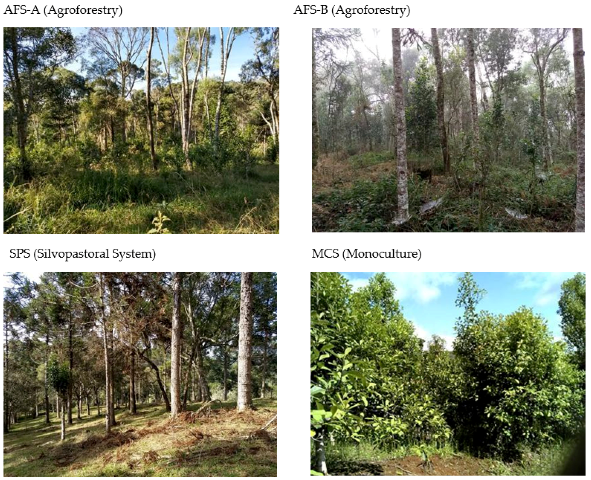
| Acronym | Altitude (m) | Geographic Coordinate | Yerba Mate Density (Trees ha−1) * | Native Tree Density (Trees ha−1) * | Notes | |
|---|---|---|---|---|---|---|
| Traditional Agroecological System in Araucaria Forest (Agroforestry System) | AFS-A | 1.030 | S 26°12′6.442″ O 51°26′32.288″ | 2000 | 388 | Area with yerba mate planted densely about 18 years ago, among native yerba mate and secondary forest in medium stage of ecological succession dominated by pioneer and early secondary forest species. No chemical inputs. |
| AFS-B | 930 | S 26°10′8.249″ O 51°21′55.547″ | - | 940 | Area with yerba mate planted densely about 15 years ago, among native yerba mate aged between 50 and 100 years, under forest vegetation that is older and denser than in AFS-A, in the middle secondary stage with dominance of Araucaria, together with pioneer and secondary species. No chemical inputs. | |
| Traditional Silvopastoral System in Araucaria Forest (Caíva) | SPS | 807 | S 26°10′8.249″ O 51°21′55.547″ | - | 236 | Area with 20 to 50 years of integrated management of native yerba mate in forest fragment with less dense Araucaria, and dairy cattle in pasture, with liming. |
| Yerba mate in Monoculture System | MCS | 938 | S 26°11′1.197″ O 51°22′13.483″ | 3.133 ** | 200 | Area with yerba mate planted in monoculture with high density, and under full sun, for about 20 years, with management and application of inputs, such as liming and mineral fertilisers. |
| Soil Ecosystem Services | Description | Soil Quality Indicators |
|---|---|---|
| Soil fertility | Capacity to provide nutrients and produce biomass [42] | pH, potential acidity (H+ + Al3+), cation exchange capacity (CEC), sum of bases (SB) |
| Carbon sequestration | Ability of soils to sequester organic carbon and promote climate mitigation services [10] | Carbon stocks (Cstock), metabolic quotient (qCO2) |
| Erosion control | Control or prevention of soil loss, provided mainly by vegetation covering the soil [22], | Bulk density (BD), granulometry (Granul), structural stability index (SSI), gravimetric soil water content (GWC) |
| Nutrient cycling | Provision of nutrients for plants and to fuel the ensemble of biological processes [42] | Litter production (LitPrd), litter nutrients (LitNut), Beta-glucosidase (Beta-Glu), urease (Ure) activities |
| Plant provision | Soil’s ability to store N and meet plant N needs [21] | Total nitrogen (TN), phosphorus (P) |
| Soil biodiversity * | Action of soil organisms that affect ecosystem functions and service provision [43] | Earthworm species richness (EwR), density (EwD) and biomass (EwB) microbial activity (FDA) |
| Soil health * | Integrative property of soil that can be changed by management [44] | Microbial activity: metabolic quotient (qCO2), microbial quotient (qMic), microbial activity (FDA), beta-glucosidase (Beta-Glu) and urease (Ure) activities |
Disclaimer/Publisher’s Note: The statements, opinions and data contained in all publications are solely those of the individual author(s) and contributor(s) and not of MDPI and/or the editor(s). MDPI and/or the editor(s) disclaim responsibility for any injury to people or property resulting from any ideas, methods, instructions or products referred to in the content. |
© 2024 by the authors. Licensee MDPI, Basel, Switzerland. This article is an open access article distributed under the terms and conditions of the Creative Commons Attribution (CC BY) license (https://creativecommons.org/licenses/by/4.0/).
Share and Cite
Parron, L.M.; Peixoto, R.T.d.G.; da Silva, K.; Brown, G.G. Traditional Yerba Mate Agroforestry Systems in Araucaria Forest in Southern Brazil Improve the Provisioning of Soil Ecosystem Services. Conservation 2024, 4, 115-138. https://doi.org/10.3390/conservation4010009
Parron LM, Peixoto RTdG, da Silva K, Brown GG. Traditional Yerba Mate Agroforestry Systems in Araucaria Forest in Southern Brazil Improve the Provisioning of Soil Ecosystem Services. Conservation. 2024; 4(1):115-138. https://doi.org/10.3390/conservation4010009
Chicago/Turabian StyleParron, Lucilia M., Ricardo Trippia dos G. Peixoto, Krisle da Silva, and George G. Brown. 2024. "Traditional Yerba Mate Agroforestry Systems in Araucaria Forest in Southern Brazil Improve the Provisioning of Soil Ecosystem Services" Conservation 4, no. 1: 115-138. https://doi.org/10.3390/conservation4010009