Striking a Balance between Conservation and Development: A Geospatial Approach to Watershed Prioritisation in the Himalayan Basin

Abstract

This study was undertaken in the Himalayan basin, in the river Lohawati, Uttarakhand, to study its hydro-morphological characteristics and prioritise the watersheds using geospatial tools. Advanced Spaceborne Thermal Emission and Reflection (ASTER-30 m) data and the Survey of India’s topographic sheets were used to analyse the study area comprehensively. Nine watersheds were identified within the basin in order to calculate the hydro-morphological characteristics in terms of basic, shape, texture, and relief aspects. The basin was identified as being elongated, with a total drainage area of 337.48 km². The interaction between the terrain, rock formations, and precipitation levels produced a branching structure in the areas drainage system that ranged from dendritic to sub-dendritic. The basin had been classified as a fifth-order basin, comprising a network of 500 stream segments spanning a total length of 492.41 km. In each of the watersheds, the primary streams are of the first order, followed by those of the second order, and so forth. The physiography and lithology of the basin have a significant influence on this pattern. The calculated elongation ratio, circulatory ratio, form factor, shape index, and shape factor ranged from 0.57 to 0.80, 0.35 to 0.64, 0.26 to 0.50, 1.98 to 3.89, and 0.57 to 1.77, respectively. These values indicate that watersheds are elongated, suggesting moderate lag times. The parameters, including drainage density (0.98 to 1.62), stream frequency (1.07 to 1.59), infiltration number (1.04 to 2.59), drainage texture (0.67 to 2.82), and drainage intensity (0.93 to 1.12), pointed towards the coarser drainage texture, higher infiltration, and minimal runoff characteristics of the basin. In light of the relief characteristics of the basin, a higher basin relief, relief ratio, and relative relief were observed for the watersheds, indicating the possibility of higher erosion and deforestation rates. Using the Weighted Sum Analysis (WSA) method, the computed factors were utilised to rank the watersheds based on their potential for erosion. Based on the WSA approach, watersheds were classified into high-, moderate-, and low-prioritisation zones. This further indicates that 36.14% (121.95 km²) of watersheds are in the high-priority zone, and that 48.84% (164.91 km²) and 15.00% (50.62 km²) of watersheds are in the moderate- and low-priority zones, respectively. The WSA is a practical strategy to prioritise watersheds when making appropriate decisions.

1. Introduction

Anthropogenic pressures and climatic changes seriously threaten global freshwater flows. Surface runoff from rain is produced using a watershed [1], which degrades the natural resources in a watershed by causing soil erosion, thereby reducing productivity and depleting groundwater levels [2]. Streams, rivers, lakes, and oceans are all affected by this discharge [3]. When managing water resources, the runoff quality and timing are extremely important. A watershed’s morphometry involves the lithological, geological, hydrological, and climatic factors that determine when runoff occurs during its regulation process. To record basin characteristics, it is imperative to employ well-established morphometric techniques, which have remained in use since the 1800s [4]. Altaf et al. [5] extensively evaluated hydrological responses using morphometric analysis, which examines surface runoff, infiltration capacity, and groundwater potential. This approach may be helpful in watersheds that are data deficient with regard to hydrology, geology, geomorphology, and soil, in accordance with [6]. Additionally, Altaf et al. [5] demonstrated that a morphometric analysis could forecast travel time, peak time, and erosional process severity. The method can be used to assess river basins to preserve their natural resources [7].

The quantification of catchment morphometry has been documented in landmark studies that have been conducted by several researchers [8,9,10,11,12,13,14]. Most of these investigations used conventional techniques, including topographic map interpretations and field observations. These characteristics are perfect for drainage studies because of their accessibility, simplicity, and low cost. Although extracting channels and catchments from topographic maps is possible, it is time-consuming because the data are not digital. Recently, it has been shown that topography-based analysis techniques and remotely sensed data are very efficient instruments for understanding and managing natural resources [15,16,17,18,19,20,21,22,23,24,25].

Sustainable development places the utmost importance on actively planning and efficiently maintaining natural resources. To manage land and water resources effectively, drainage basins, catchments, and sub-catchments should be incorporated as fundamental units [26]. Moreover, the conservation and judicious use of all relevant resources are prioritised by watershed management in order to maximise output while minimising environmental effects [27]. The effective management of watersheds can help mitigate the impact of natural disasters, such as floods and droughts, and it addresses issues like excessive runoff, increased soil erosion, and insufficient infiltration [28]. Unfortunately, many mountain watersheds face catastrophic situations due to human activities, such as deforestation, urbanisation, shifting cultivation, and other land uses that do not support sustainability. Thorough management plans are required to develop these watersheds sustainably by implementing effective strategies for resource conservation, pollution control, ecosystem restoration, and community engagement.

The prioritisation of sub-watersheds is made possible through morphometric analysis, even when a soil map is not available [29]. Sub-watershed prioritisation significantly depends on the morphological characteristics of each watershed. It is used to identify hotspots that threaten the natural ecological system in both overt and covert ways, as well as for management objectives [14]. The use of linear, areal, and relief parameters makes it possible to uncover the various geographical and geomorphological aspects of a river basin. These parameters also determine direct or indirect connections between these features, surface runoff, and soil erosion susceptibility.

Consequently, it is possible to locate and prioritise soil-erosion-prone areas within a watershed [30,31]. As part of watershed management, it is necessary to prioritise watersheds in terms of cost, project type, and development programs. When prioritising sub-watersheds, we may consider their impact on runoff, as well as the frequency and severity of flooding, the creation rate of groundwater resources, and the rate of soil erosion. Mustak et al. [32] suggests a technique for prioritising sub-watersheds by assessing and ranking them in accordance with the extent of soil erosion and the significance of their drainage areas. Various factors, including soil loss, land utilisation, land cover, morphometric features, and the socioeconomic status of the population, among other relevant considerations, can be employed for sub-watershed prioritisation.

Geospatial statistical techniques have been employed in various endeavours to analyse and prioritise sub-watersheds across different scales, such as Multicriteria Decision Analysis [33,34,35,36,37,38,39], Weighted Sum Analysis [40,41,42], as well as the Sediment Yield Index [43,44,45,46,47,48,49,50,51], Principal Component Analysis [52,53,54], and Compound Factor analysis [55,56,57,58]. Previous studies have demonstrated that the Weighted Sum Analysis (WSA) technique [40] is highly effective in prioritising sub-watersheds, especially regions with limited data or lacking stream gauges. The method’s strength lies in its ability to ensure consistency during the prioritisation process when criteria and weights are defined objectively, based on reliable data and expert knowledge, thus reducing the subjectivity commonly found in other methods [40]. Further, the WSA method offers adaptability to different contexts and decision-making scenarios. By analysing various morphometric parameters, such as linear, areal, and relief, aspects, and utilising digital elevation models (DEM), the WSA method streamlines the sub-watershed prioritisation process. The present study showcases the practical application of the Weighted Sum Analysis (WSA) technique for the efficient prioritisation of sub-watersheds, even in regions with limited data and that are inaccessible.

To date, there has been a noticeable absence of comprehensive research on the analysis and prioritisation of watersheds in the Lohawati basin. This noticeable gap in knowledge creates a crucial need to address the issues of prioritising watersheds based on their stability regarding land erosion, which is of the utmost importance for adequate soil and watershed management. Consequently, undertaking a focused study on prioritising watersheds within the study area becomes essential. This research aims to fill the void resulting from the lack of any investigation and is poised to become a fundamental cornerstone for making informed decisions regarding the allocation of watershed management and conservation resources. The primary objective of this study was to conduct a morphometric analysis of the Himalayan basin. This study also aimed to employ geospatial and statistical methods, along with remote sensing and GIS techniques, to prioritise sub-watersheds based on the derived variables. Despite challenges in recording critical variables due to the study area’s location at the Indo-Nepal border, this research emphasises the importance of using alternative methods while adhering to scientific principles. WSA, based on digital elevation models, effectively analysed morphometric parameters, like shape, texture, and relief, to guide watershed management planning without complex models. When the direct measurement of variables, like sediment yield, are complicated, this study highlights the value of employing indirect indicators and proxy data for assessing erosion susceptibility and guiding conservation efforts. This research proposes alternative ways to approximate essential variables by employing scientific principles and statistical techniques, providing valuable insights for watershed management decision making and resource allocation. Moreover, this research aims to set a foundation for geomorphometric parameters and their association with the vulnerability of watersheds to erosion risks. This information serves as a guide for conservation projects and programs in sub-watersheds with limited financial resources.

2. Materials and Methods

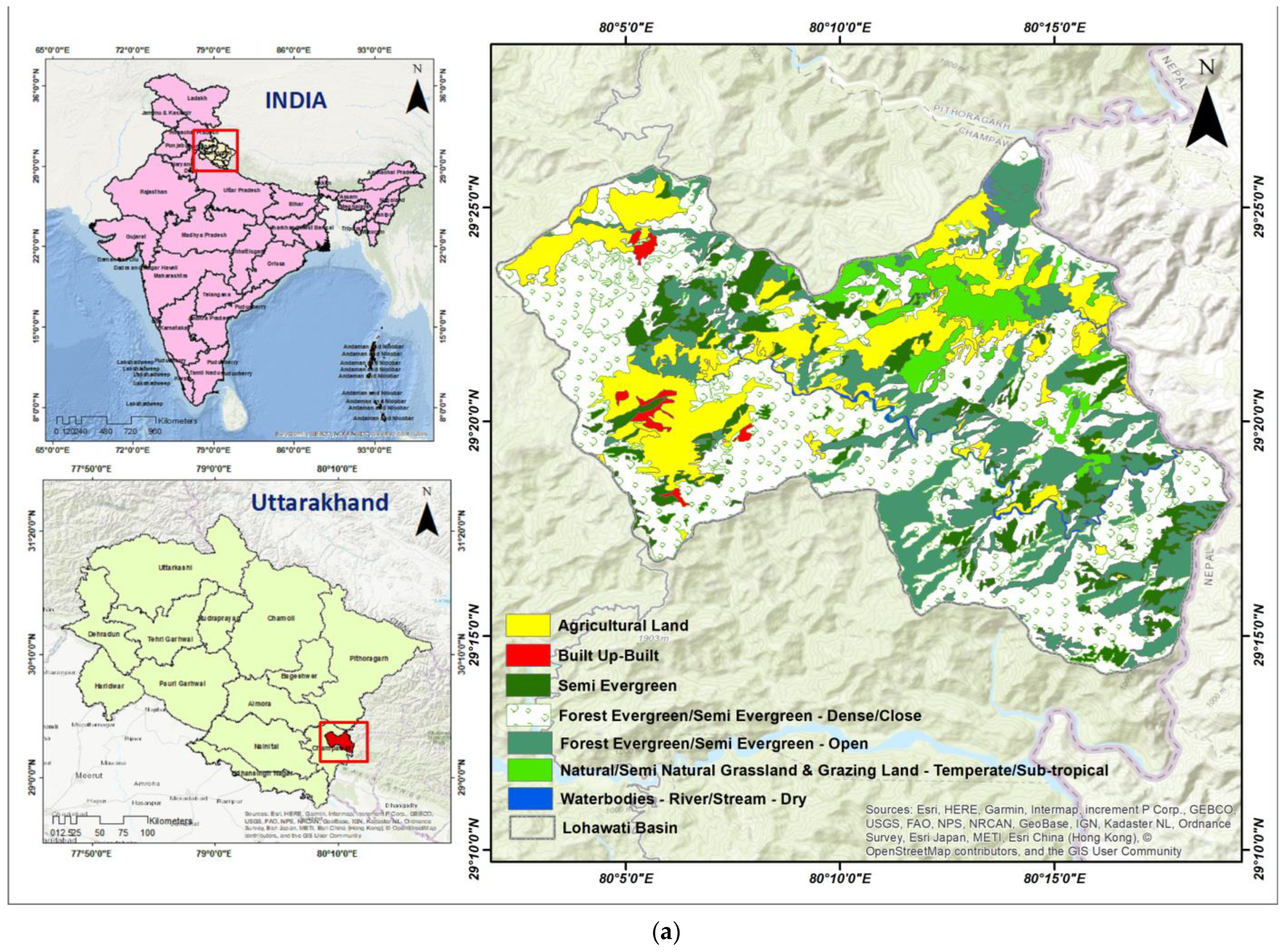
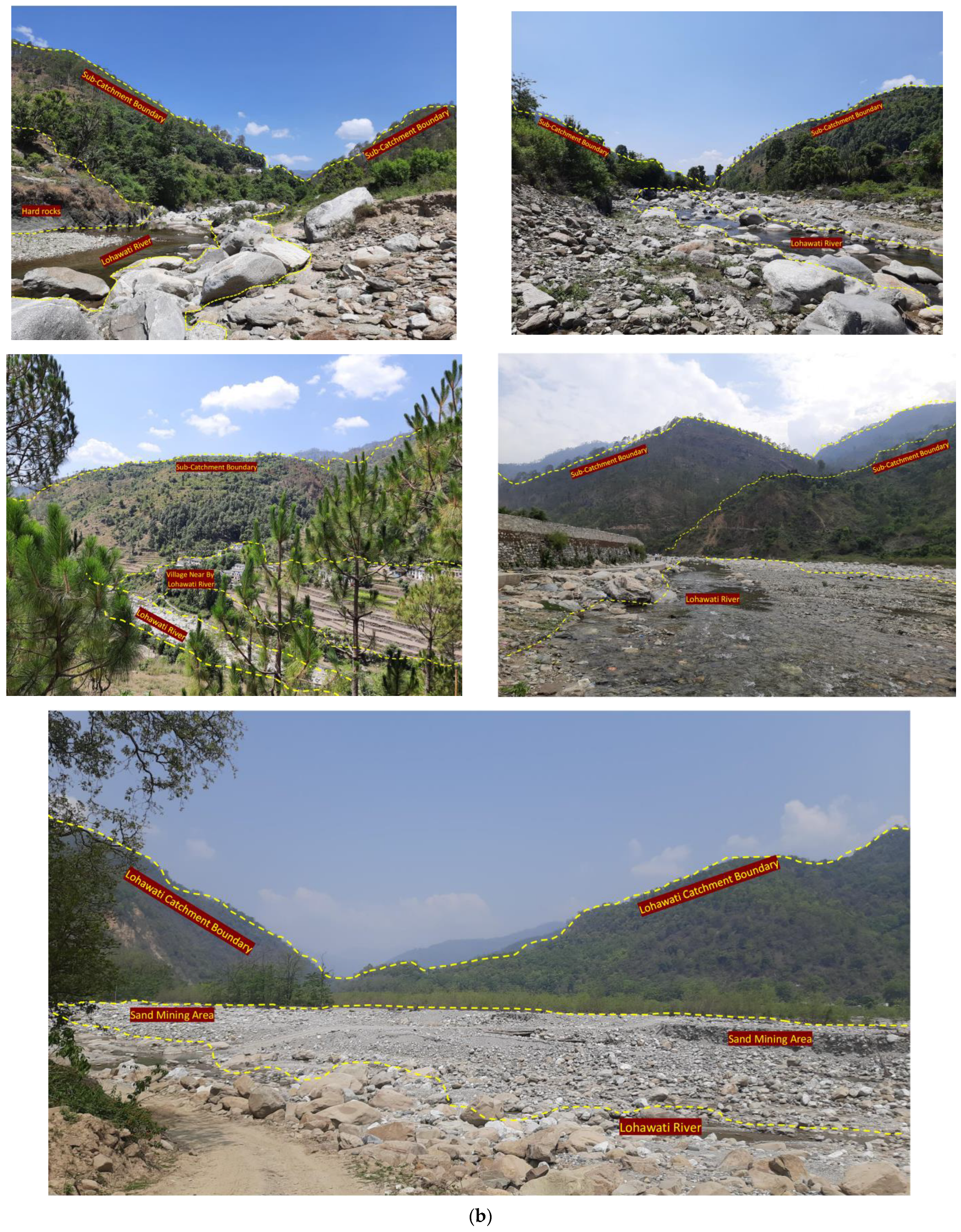
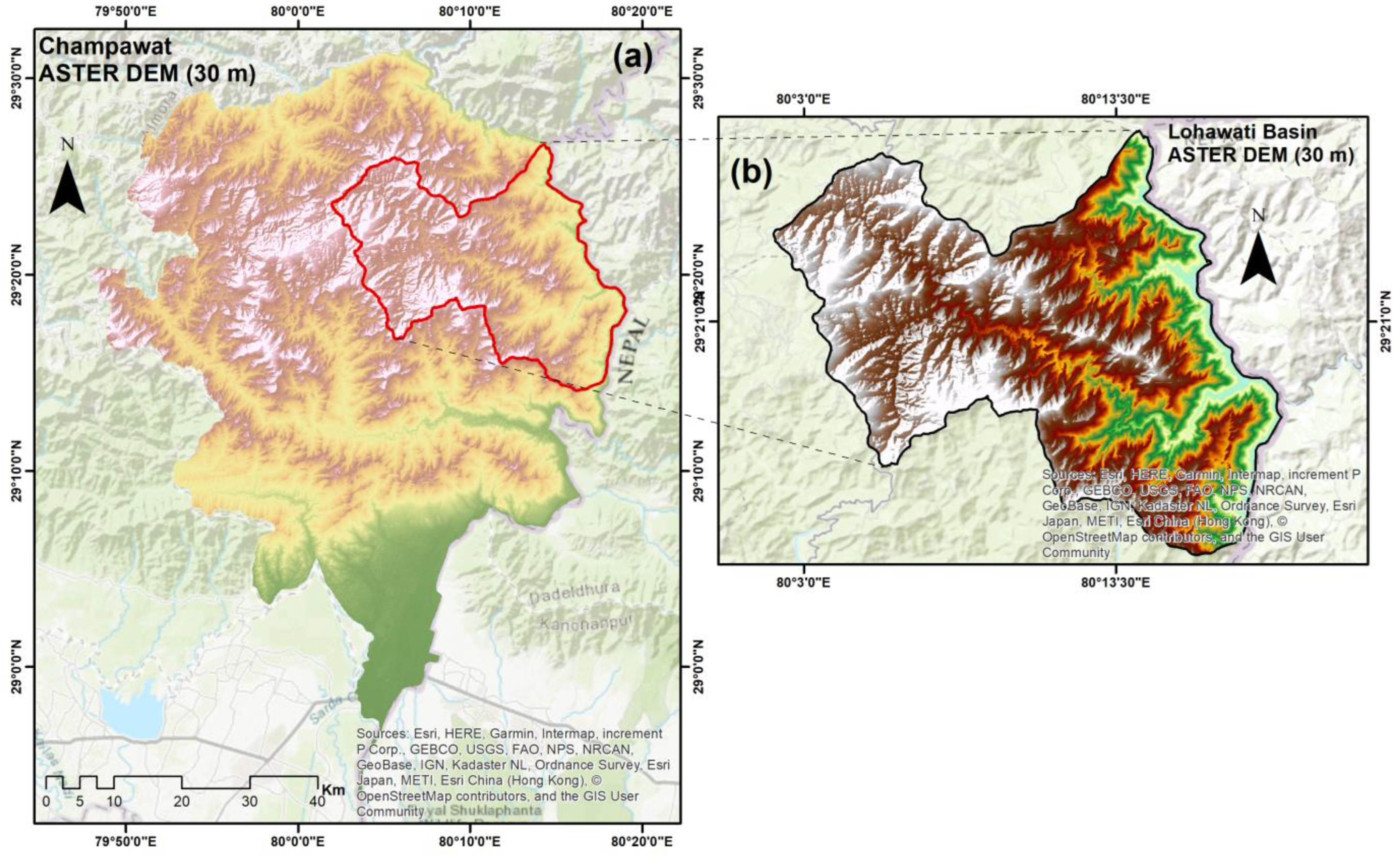
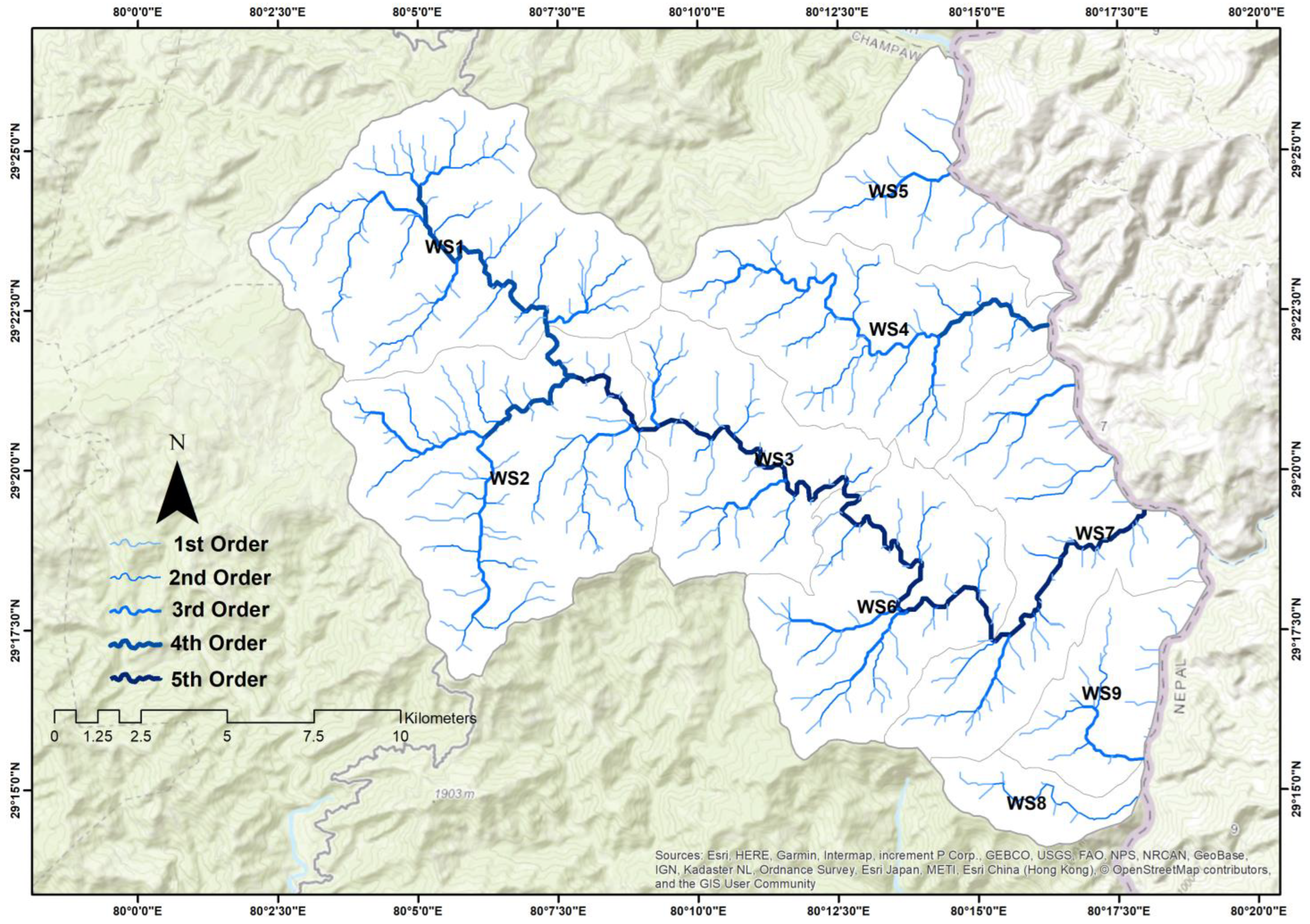
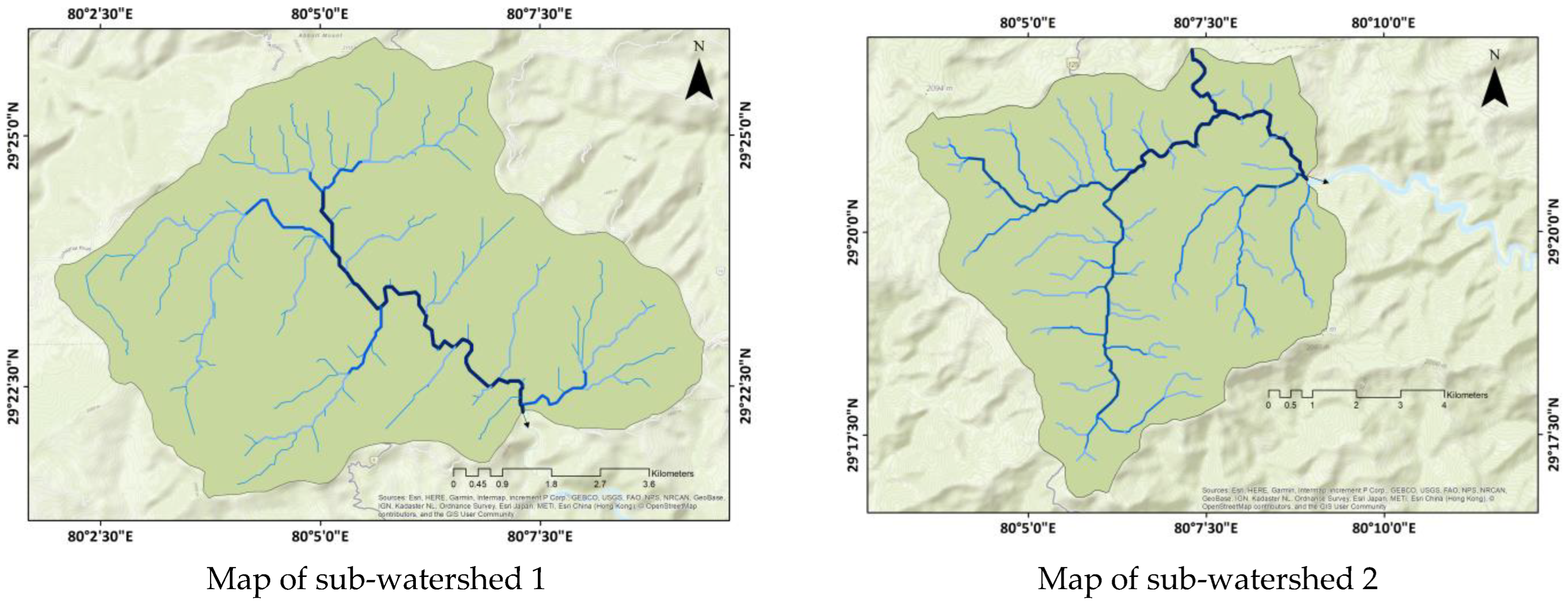
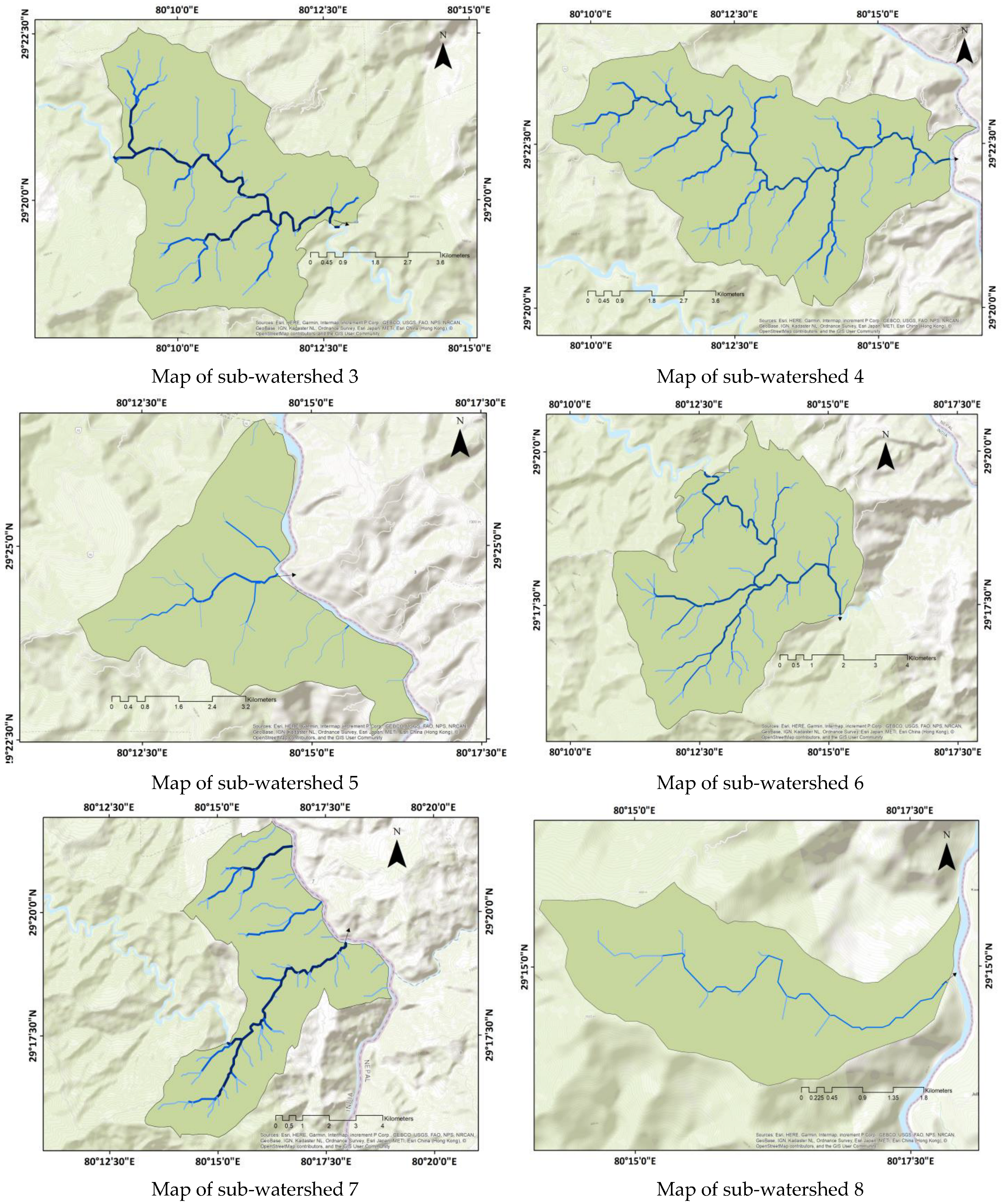
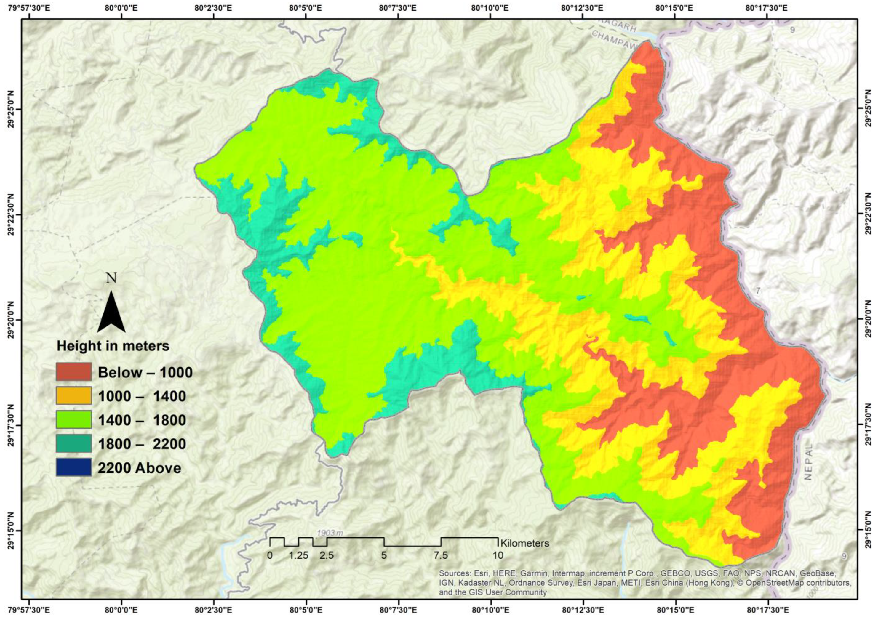
2.1. Description of Study Site

The study area spans from 29°26′30′′ N; 80°3′30′′ E to 29°15′30′′ N 80°20′0′′ E in the Kumaon district of eastern Uttarakhand, India (Figure 1a,b). The Lohawati, a major river that cuts across the basin, is responsible for the basin’s appellation. The river flows from Bansaur Kila in the west to the east for about 10 km before reaching Lohaghat. Valleys and hills are dotted over the exceedingly rugged environment all along its length. A prevalent evergreen forest particularly characterises the middle and lower sections of the basin. Agriculture is practiced irregularly in the basin’s upper section, i.e., near the source. Lohaghat, the largest settlement along the river’s edge, has the maximum inhabitation. The residents frequently perform religious rituals along the riverbanks, close to the city. Water for both human and agricultural use is drawn from the river. Many tributaries flow into the river at various spots. The water level in the river has been dropping for multiple reasons, including continuing water withdrawals for domestic and agricultural use, insufficient recharge from precipitation, and others. The river begins its long journey through the Himalayas, passing through picturesque valleys, narrow gorges, villages, and finally, the Indo-Nepal border at Tamli, where it joins the River Mahakali.

The geological configuration of the area is highly intricate, resulting from numerous tectonic disturbances, caused by different orogenic cycles [59]. The exposed rock succession in the region belongs to the Almora group of rocks, which includes formations like Salla, Gorakhnath, Gumalikheth, and the Champawat granodiorite. The prominent rock types found in this group comprise pale-green-to-cream-colored quartzite, along with chlorite schist, phyllite, metabasitic rocks, and garnetiferous biotite mica schist, often interspersed with quartzite layers [60].

The sub-tropical highland climate is the Koppen-Geiger description for this area (Cwb). The warmest months are April, May, and June, while the coldest are December and January. Factors like elevation, latitude, and sunshine hours majorly shape the local climate. The warmest month is June (avg temp 21.8 °C), and the coldest is December (avg temp 9.1 °C), with an annual average temperature of 16.6 °C. The degree of fluctuation in the yearly temperature is approximately 12.7 °C. Sometimes, heavy precipitation during the harsh winters (December to March) is characterised by snowfall. From June to October, the monsoon season brings a wide range of precipitation, with the average being 3752 mm annually. July receives the highest rainfall (avg 965 mm), while November gets the least rainfall (avg 21 mm). More significant amounts of precipitation are typically seen during summer than winter. The time before the annual monsoon rains begin is the driest [61] (https://mausam.imd.gov.in accessed on 25 September 2022).

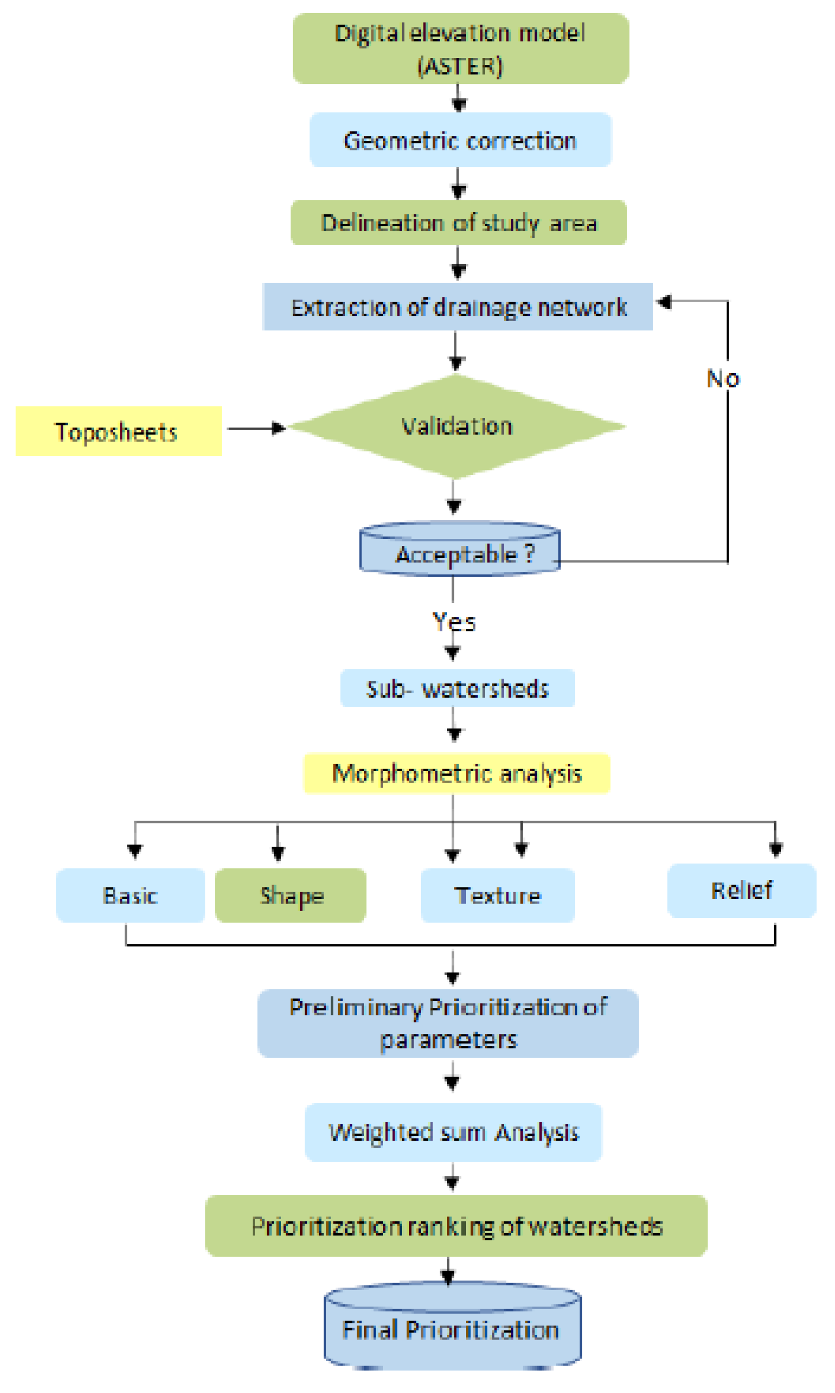
2.2. Data Used and Methodology

In this study, we evaluated the region’s morphology by dividing the study area into sub-watersheds to identify and prioritise areas prone to soil erosion. To conduct a quantitative morphometric analysis, we utilised ASTER GDEM-30 m. Additionally, we employed the Survey of India topographic maps (1:50,000) to verify and analyse the drainage network. Various morphometric metrics, including basic, shape, texture, and relief elements of the study area, were identified from the analysed DEM. These measurements were subsequently validated by comparing them to the topographical maps from the Survey of India (1:50,000), specifically the 62C3, 62C4, and 62C7 maps. The detailed information about the data utilised in the research is documented in

Table 1. Information about the data utilised in the research.

S. No.	Data Type	Details of Data	Source
1.	ASTER GDEM	30 m resolution	http://demex.cr.usgs.gov/DEMEX/. (accessed on 5 July 2022)
2.	SOI toposheets	62C3, 62C4, and 62C7.	Survey of India, Dehradun, Uttarakhand, India

.

2.3. ASTER-30 m

The National Aeronautics and Space Administration (NASA) of the United States and Japan’s Ministry of Economy, Trade, and Industry (METI) have worked together to create the ASTER GDEM. The ASTER sensor, installed on the Terra satellite, was disconnected in December 1999. It consists of nadir- and backward-viewing telescopes that can record stereo images with a base-to-height ratio of 0.6 at a viewing angle of 27.7 degrees (3B) in the near-infrared spectral band 3N. The GDEM output is generated by automatically processing 1.5 million stereo pairs using stereo correlation methodology. While the computed DEM has a resolution of 30 m, bands 3N and 3B have a higher resolution of 15 m. The GDEM covers the entire area between 83 degrees north and 83 degrees south latitude [62]. Each ASTER scene measures 4100 by 4200 pixels or approximately 60 by 60 km on the Earth’s surface in the visible or near-infrared range. It has a spatial resolution of 1 arc-second for latitude and longitude (~30 m) and a vertical accuracy of around 10 m [62]. In this study, ASTER GDEM version-2 was obtained from the http://demex.cr.usgs.gov/DEMEX/ (accessed on 5 July 2022) (Figure 2).

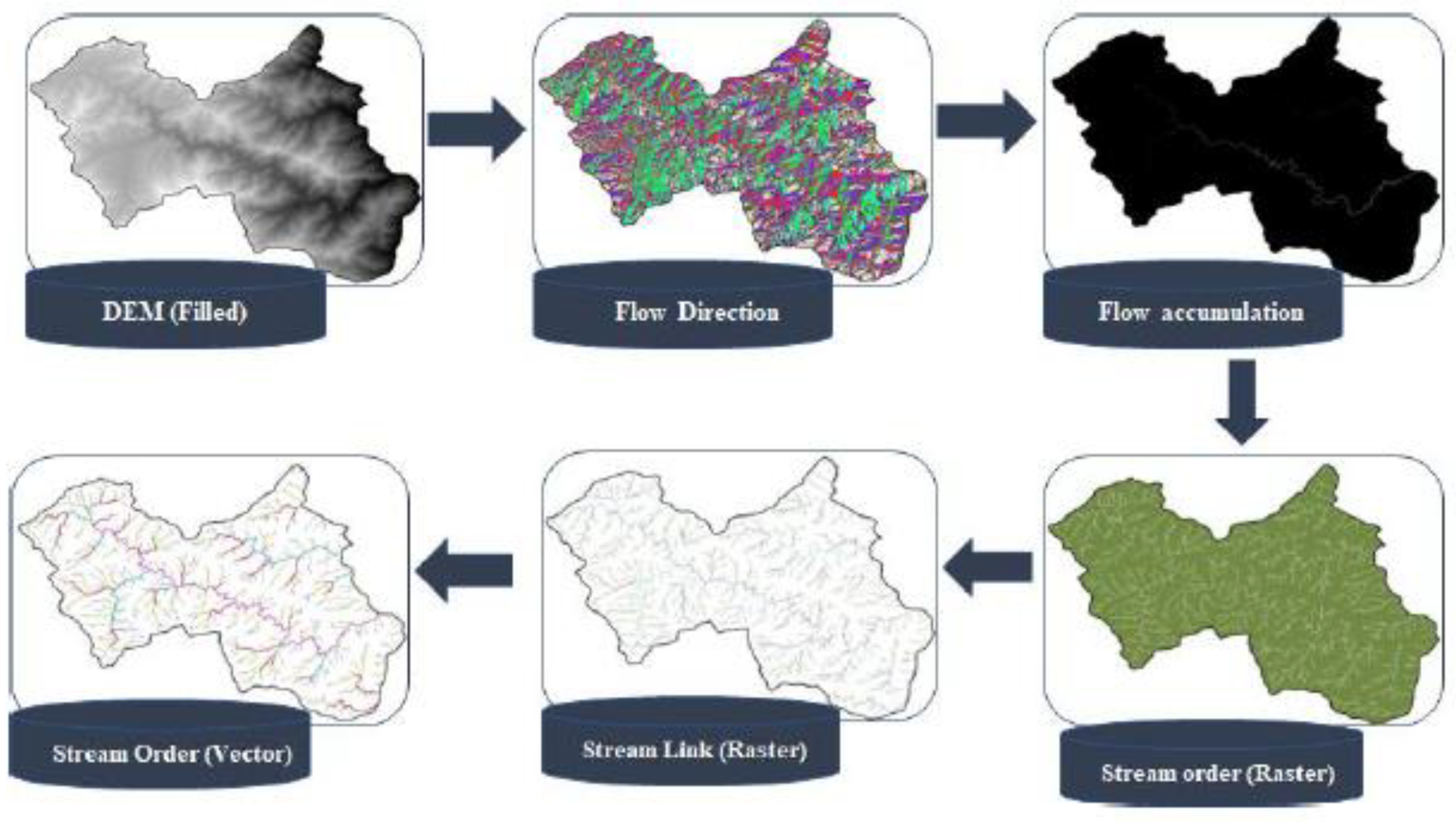
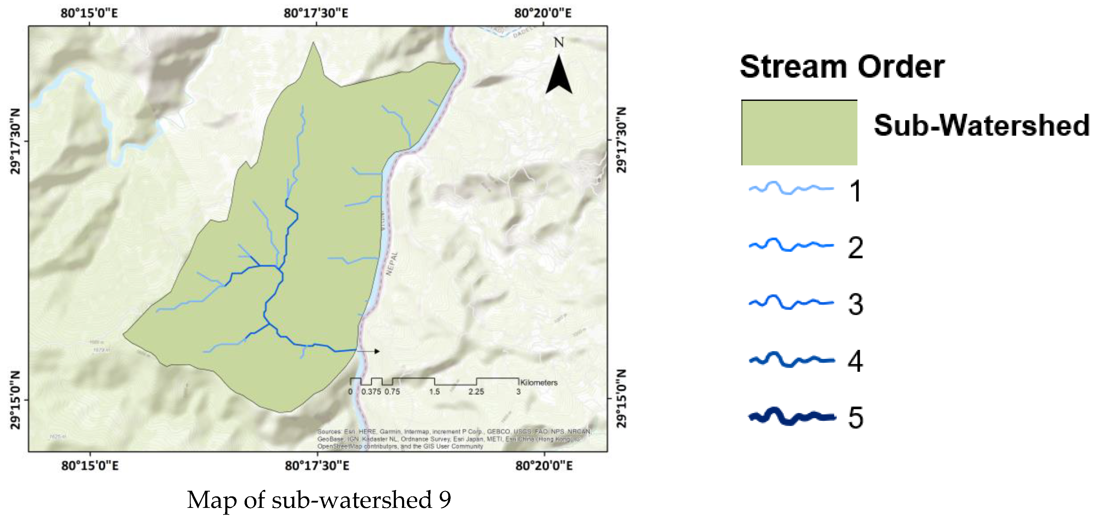
2.4. Extraction of Drainage Network

After careful examination of the DEM data, we reproject it onto a Universal Transverse Mercator (zone 43) projection, ensuring the usage of uniform measurement units across all axes. Subsequently, we utilised a void-filling algorithm, powered by the Map Algebra tool of the Spatial Analyst extension of ArcGIS 10.8, to address the gaps existing in the downstream segment of the Lohawati basin. We successfully extracted the drainage networks and the basin boundary from the ASTER DEM by leveraging the hydrological capabilities in the Spatial Analyst add-on for ArcGIS 10.8.

In this study, we utilised the D8 methodology to organise the drainage network hierarchically. This method involves using a hydrological tool in ArcGIS and working with a high-resolution dataset (30 m) [63,64]. We performed several steps to create the drainage network, including pixel filling, estimating flow direction and accumulation, and identifying the area where water flows into an output grid cell. We used a “cell threshold” setting to decide how many raster cells are needed in a drainage network to start a stream grid (Figure 3). For this study, we set the threshold to 200 pixels to create the stream network. Then, we converted the raster data into a feature representation to reconstruct the drainage layer. The stream segments were then ordered using the Strahler (1964) stream ordering method [14]. To verify the accuracy of the drainage network derived from the dataset, we compared it to the information from the SOI toposheets. The boundary of the watershed was determined based on the point where all the water in the entire watershed flows into the river. The length and area of the watershed were calculated by using the geometric properties of the generated polygons.

2.5. Calculation of Morphometric Characteristics

The morphometric features of the study area were analysed using the mathematical equations outlined in

Table 2. The mathematical equations used to measure the morphometric parameters quantitatively.

Morphometric Parameters	Symbol	Formula	References
Basic parameters
Basin area (km2)	A	GIS software (ArcGIS 10.8) analysis	[11]
Basin perimeter (km)	P	GIS software (ArcGIS 10.8) analysis	[11]
Basin length (km)	Lb	1.312 × A0.568	[11]
		Where Lb = basin length
		A = basin area (km2)
Stream number	Nu	Number of stream segments	[12]
Stream order	U	Hierarchical rank	[14]
Stream length (km)	Lu	Length of the stream segment	[65]
Mean stream length	Lsm	Lsm = Lu/Nu	[14]
		Where Lsm = mean stream length
		Lu = total stream length of order “u”
		Nu = total no. of stream segments of order “u”
Stream length ratio	Rl	Rl = Lu/Lu-1	[65]
		Where Rl = stream length ratio
		Lu = total stream length of order “u”
		Lu-1 = total stream length of its next lower-order
Shape parameters
Form factor	Ff	Ff = A/Lb2	[9]
		Where Ff = form factor
		A = area of the basin (km2)
		Lb2 = square of basin length (km)
Circulatory ratio	Rc	Rc = 4 × Pi × A/P2	[10]
		Where Rc = circulatory ratio
		Pi = “Pi” value, i.e., 3.14
		A = area of the basin (km2)
		P = perimeter (km)
Elongation ratio	Re	Re = 2v (A/Pi/Lb)	[13]
		Where Re = elongation ratio
		Pi = “Pi” value, i.e., 3.14
		A = area of the basin (km2)
		Lb = basin length (km)
Shape index	Si	Si = Lb2/A	[65]
		Where Si = shape index
		Lb = basin length
		A = area of basin
Shape factor	Sf	Sf = Pu/Pc	[66]
		Where Sf = shape factor
		Pu = perimeter of the circle of watershed area
		Pc = perimeter of watershed
Texture parameters
Length of overland flow (km)	Lg	Lg = 1/2 (Dd)	[65]
		Where Lg = length of overland flow
		Dd = drainage density
Drainage density (km km−2)	Dd	Dd = Lu/A	[9]
		Where Dd = drainage density
		Lu = total stream length of order “u”
		A = area of the basin (km2)
Bifurcation ratio	Rb	Rb = Nu/Nu + 1	[11]
		Where Rb = bifurcation ratio
		Nu = total no. of stream segments of order “u”
		Nu + 1 = number of segments of the next higher-order
Mean bifurcation ratio	Rbm	Average of bifurcation ratio of all orders	[13]
Stream frequency (km−2)	Fs	Fs = Nu/A	[9]
		Where Fs = stream frequency
		Nu = total no. of streams of all orders
		A = area of the basin (km2)
Constant of channel maintenance (km2 km−1)	C	C = 1/Dd	[11]
		Where C = constant of channel maintenance
		Dd = drainage density
Drainage intensity	Di	Di = Fs/Dd	[28,67]
		Where Di = drainage Intensity
		Fs = stream frequency
		Dd = drainage density
Infiltration number	If	If = Fs × Dd	[67]
		Where If = infiltration number
		Fs = stream frequency
		Dd = drainage density
Texture ratio	Rt	Rt = N1/P	[11]
		Where Rt = texture ratio
		N1 = number of 1st order streams
		P = basin perimeter (km)
Drainage texture	Dt	Dt = Nu/P	[65]
		Where Dt = drainage texture
		Nu = total number of streams
		P = perimeter (km)
Compactness coefficient	Cc	Cc = Pc/Pu	[68]
		Where Pc = perimeter of watershed
		Pu = perimeter of the circle of watershed area
Relief parameters
Height of basin mouth (km)	z	GIS analysis/DEM
Maximum height of the basin (km)	Z	GIS analysis/DEM
Total basin relief (km)	H	H = Z − z	[12]
		Where H = total basin relief
		Z = maximum height of the basin (km)
		z = height of basin mouth (km)
Relief ratio	Rh	Rh = H/Lb	[11]
		Where Rh = relief ratio
		H = total relief of the basin (km)
		Lb = basin length (km)
Relative relief	Rr	Rr = 100 H/P	[11]
		Where Rr = relative relief
		H = total relief of the basin (km)
		P = perimeter (km)
Ruggedness number	Rn	Rn = Dd ×H	[14]
		Where Rn = ruggedness number
		Dd = drainage density
		H = total basin relief (km)

. These metrics provide valuable insight into the basin’s physiographic features and can aid in prioritising watersheds for management and conservation purposes.

2.6. Prioritisation of Sub-Watersheds

The Weighted Sum Analysis (WSA) method was utilised for the analysis. This technique, developed by [40], uses geospatial technology in combination with statistical methods to determine the relative significance of each parameter and provide appropriate weights. The method avoids the biases commonly present in many watershed prioritisation methods.

The WSA method is a precise statistical technique that employs geospatial technology to determine which parameter should be considered in the final analysis. The method determines the relative importance of each parameter using statistical correlation and assigns weights to each parameter accordingly (Equation (1)) [40]. The method provides a comprehensive and unbiased approach to prioritising watersheds, ensuring that all critical factors are considered.

$$\mathrm{Prioritization}={\sum }_{i=1}^n{W}_i\times X_i$$

(1)

where W_i is the weighted average of each morphometric parameter, and X_i is the value of morphometric parameters determined using the WSA technique. The strategy mentioned above can identify the components’ effectiveness and consider each impact separately.

A preliminary ranking of the selected morphometric characteristics was performed to prioritise the Lohawati basin’s watersheds. The linear and relief factors directly correlate with soil erosion, whereas the aerial parameters have an inverse correlation. Consequently, morphometric parameters with greater values, such as linear and relief factors, are assigned higher ranks, indicating an increased susceptibility to erosion. Conversely, areal parameters with higher values receive lower ranks, suggesting a reduced risk of soil erosion. The ranking system reflects the significance of morphometric factors in influencing erosion susceptibility, with higher ranks indicating a more significant risk and vice versa [49,69,70].

First, a correlation matrix was created to examine the relationship between selected morphometric variables. Then, the total correlation for each selected variable was calculated. To determine the final weights for each parameter, the sum of correlation coefficients for each parameter was divided by the overall correlation total. Next, a model (Equation (1)) was developed to assess the priority of each parameter by assigning calculated weights to them. The prioritisation values for all the sub-watersheds were computed based on the weighted averages of the selected morphometric components. The detailed methodology followed for prioritising watersheds is given in Figure 4.

3. Results and Discussion

The current study’s investigation parameters were computed by employing various techniques suggested by different researchers, with their corresponding formulae listed in the appropriate sections. The computed morphometric variables are presented in

Table 3. Basic morphometric parameters of the Lohawati Sub-basins.

(a)
Code	Basin Length (km)	Basin Area (km2)	Basin Perimeter (km)	Stream Order					Total Stream Numbers	Stream Length (km)					Total Stream Length (km)
				U1	U2	U3	U4	U5		LU1	LU2	LU3	LU4	LU5
WS1	12.00	59.87	34.37	71	18	5	1		95	46.78	29.43	7.92	10.37		94.50
WS2	11.10	62.08	35.07	74	19	3	2	1	99	50.22	26.30	13.32	7.27	3.67	100.78
WS3	9.45	34.89	29.94	43	9	2		1	55	25.96	11.62	4.41		11.76	53.75
WS4	11.31	45.57	35.30	55	14	1	1		71	27.30	20.96	13.72	4.67		66.65
WS5	7.43	23.42	28.13	20	4	1			25	14.62	5.50	2.80			22.92
WS6	9.60	40.66	31.62	45	9	2		1	57	28.44	12.60	7.00		13.33	61.37
WS7	13.00	43.76	39.87	52	11	1	1		65	33.82	13.27	5.38	8.79		61.26
WS8	6.00	9.26	16.38	9	1	1			11	3.87	6.64	1.07			11.58
WS9	7.65	17.93	20.83	17	4	1			22	12.28	3.54	3.78			19.6
(b)
Code	Mean Stream Length								Mean Stream Length (km)	Stream Length Ratio
	LU1/NU1	LU2/NU2		LU3/NU3	LU4/NU4	LU5/NU5				LU2/LU1	LU3/LU2	LU4/LU3	LU5/LU4
WS1	0.66	1.64		1.58	10.37				1.99	0.63	0.27	1.31
WS2	0.68	1.38		4.44	3.635	3.67			1.76	0.52	0.51	0.55	0.50
WS3	0.60	1.29				11.76			1.93	0.45	0.38
WS4	0.50	1.50		13.72	4.67				1.86	0.77	0.65	0.34
WS5	0.73	1.38							1.07	0.38	0.51
WS6	0.63	1.40				13.33			2.09	0.44	0.56
WS7	0.65	1.21			8.79				1.62	0.39	0.41	1.63
WS8	0.43								6.24	1.72
WS9	1.47	2.89							1.83	0.29	1.06

,

Table 4. Shape morphometric parameters of the Lohawati sub-basins.

Code	Elongation Ratio	Circulatory Ratio	Form Factor	Shape Index	Shape Factor
WS1	0.73	0.64	0.42	2.41	1.74
WS2	0.80	0.63	0.50	1.98	1.77
WS3	0.71	0.49	0.39	2.56	1.17
WS4	0.67	0.46	0.36	2.81	1.29
WS5	0.74	0.37	0.42	2.36	0.83
WS6	0.75	0.51	0.44	2.27	1.29
WS7	0.57	0.35	0.26	3.86	1.10
WS8	0.57	0.43	0.26	3.89	0.57
WS9	0.62	0.52	0.31	3.26	0.86

and

Table 5. Texture morphometric parameters of the Lohawati sub-basins.

Code	Stream Frequency (km−2)	Drainage Density (km km−2)	Bifurcation Ratio				Mean Bifurcation Ratio	Infiltration Number	Constant of Channel Maintenance (km2 km−1)	Length of Overland Flow (km)	Drainage Intensity	Texture Ratio	Drainage Texture	Compactness Coefficient
			NU1/ NU2	NU2/ NU3	NU3/ NU4	NU4/ NU5
WS1	1.59	1.58	3.94	3.60	5		3.14	2.50	0.63	0.79	1.01	2.07	2.76	0.57
WS2	1.59	1.62	3.89	6.33	1.5	2	3.43	2.59	0.62	0.81	0.98	2.11	2.82	0.56
WS3	1.58	1.54	4.78	4.50			2.32	2.43	0.65	0.77	1.02	1.44	1.84	0.86
WS4	1.56	1.46	3.93	14.00	1		4.73	2.28	0.68	0.73	1.07	1.56	2.01	0.77
WS5	1.07	0.98	5.00	4.00			2.25	1.04	1.02	0.49	1.09	0.71	0.89	1.20
WS6	1.40	1.51	5.00	4.50			2.38	2.12	0.66	0.75	0.93	1.42	1.80	0.78
WS7	1.49	1.40	4.73	11.00	1		4.18	2.08	0.71	0.70	1.06	1.30	1.63	0.91
WS8	1.19	1.25	9.00	1.00			2.50	1.49	0.80	0.63	0.95	0.55	0.67	1.77
WS9	1.23	1.09	4.25	4.00			2.06	1.34	0.91	0.55	1.12	0.82	1.06	1.16

. The drainage area of the Lohawati basin encompasses a vast expanse of 337.48 km², with its drainage pattern being dendritic to sub-dendritic (Figure 5). The region’s terrain features, geomorphology, and precipitation conditions are critical in shaping the basin’s drainage pattern. Additionally, the Lohawati River is categorised as a basin ranging from first to fifth order, which is determined by the order of its streams.

3.1. Basic Morphometric Parameters

The basic morphometric parameters, estimated for the study area, are given in Table 3. The basin length is the longest dimension running parallel to the primary drainage [11] and was found to be the highest in WS7 (13 km), and the lowest in WS8 (6 km). The basin length of other watersheds lies between these two extremes, with lengths indicating that the basins are smaller. The size of the basin area plays a crucial role in defining the basin’s overall geometry. WS2 had the largest basin area, measuring 62.08 km², while WS8 had the smallest basin area, covering only 9.26 km². The basin perimeter gives information about the extent and form of the basin. The largest perimeter was obtained for WS7 (39.87 km), and the smallest was obtained for WS8 (16.38 km). Stream order, which indicates the basin’s size and scale, was calculated according to [13] (Figure 6). The Lohawati basin was categorised as a 5th-order basin with 500 stream segments. The largest number of stream segments was found in WS2 (99), while the lowest was found in WS8 (11).

Moreover, across all the watersheds, maximum stream segments were observed to be in the first order, followed by the second order, and so forth (Table 3). This observation aligns with Horton’s law [9,65]. The stream numbers further indicated that WS1 and WS2 were relatively more permeable than the remaining watersheds. According to [71], increasing discharge and velocity are related to increased stream order. We can infer that the differences in the physical characteristics of the watersheds lead to varying sediment loads and water flow contributions. As mentioned by [25], any deviation from Horton’s rule suggested that the basin had a rugged terrain with gentle slopes, diverse rock types, and possibly experienced uplift events. This implies that the Lohawati basin’s subsurface landscape was lithologically uniform throughout and showed no signs of geological uplift because no such divergence was found in our study.

The total stream length obtained for the Lohawati basin was 492.41 km, ranging from 11.58 km in WS8 to 100.78 km in WS2 (Table 3). According to the Horton’s Law of stream length, each stream order’s mean length increases geometrically with increasing stream order. An analogous trend was seen in the Lohawati basin’s watersheds (Table 3), indicating the basin’s homogeneous development. The stream length ratio (R_l) was determined by dividing the length of a stream segment for a specific order (Lu) by the length of the stream segment for the previous order (Lu-1). The “R_l” increased from lower to higher stream orders, as indicated by the “R_l” between various sub-watersheds, and this indicates that streams are at a developed geomorphic stage (Table 3). In WS1, the third- to second-order stream length ratio was 0.27, while in WS8, the second- to first-order stream length ratio was 1.72. The “R_l” between consecutive stream orders changes due to differences in slope and topographic conditions. Moreover, this ratio is strongly linked to the basin’s surface flow discharge and erosional stage [72].

3.2. Shape Morphometric Parameters

Area (A), perimeter (P), and basin length (Lb) are three of the most essential morphometric variables used to represent the basin’s shape [10,11,65]. Forecasting the hydrological behaviour of a basin requires knowledge of its shape, which can be expressed in terms of the form factor (Ff), elongation ratio (Re), circulatory ratio (Rc), shape index (Si), and shape factor (Sf) [65,73].

The elongation ratio (Re) is used to assess the shape of a watershed. It represents how stretched or elongated the watershed is, which is computed by dividing the longest length of the watershed by the diameter of a circle with the same area. This ratio helps categorise the different slopes of watersheds or basins. The Lohawati basin’s elongation ratio, given in Table 4, varied from 0.57 in WS7 and WS8 to 0.80 in WS2. According to [11], an elongation ratio of 0.9–1.0 represents a circular shape, 0.8–0.9 represents an oval shape, 0.7–0.8 represents less elongated shapes, 0.5–0.7 represents elongated shapes, and a value below 0.5 represents more elongated shapes. The watersheds WS4, WS7, WS8, and WS9 had elongated shapes with an Re between 0.5 and 0.7, while WS1, WS2, WS3, WS5, and WS6 had less elongated shapes, with an Re between 0.7 and 0.8. The “Re” value tends to approach 1.0 when the basin shape is closer to a circle. It typically ranges from 0.6 to 1.0 under various geological and climatological conditions [14]. According to Dar et al. [74], values closer to 1.0 are associated with gentle terrain, limited or insignificant structural effects, intense infiltration, and runoff. On the other hand, [14] pointed out that values between 0.8 and 0.6 are linked to steep gradients and high relief. Since the “Re” values of the watersheds fall between 0.6 and 0.8, it suggests that they have steep slopes and high relief. This makes them more susceptible to soil erosion [75].

The circulatory ratio (Rc) is a metric used to evaluate the shape of a basin quantitatively. The computation involves dividing the basin’s area by the diameter of a circle that has the same perimeter as the basin [10,14]. Among the watersheds, WS7 had the lowest “Rc” value (0.35), while WS1 had the highest “Rc” value (0.64) (Table 4). Various basin characteristics, such as stream length and frequency, geological structures, land use/cover, climate, relief, and basin slope, can influence this measurement [76]. Findings from [77] demonstrated a robust correlation between “Rc” and structural disturbances, suggesting that basins with low “Rc” values generally experienced minimal structural disruptions, while higher “Rc” values were associated with more significant disturbances. The “Rc” values of the watersheds suggested that WS1 and WS2 had moderate structural disturbances, while the remaining watersheds are subject to low structural disturbances (Table 4).

Horton [65] states that a form factor is employed to evaluate the flow intensity in basins of a specific size. The form factor of the Lohawati basin’s sub-watersheds ranged from 0.26 in WS7 and WS8 to 0.50 in WS2 (Table 4). As per [9,10], the form factor indicates the basin shape, with a smaller value indicating a more elongated shape and a larger value indicating a tendency towards circularity. The Lohawati basin’s watersheds have relatively smaller “F_f” values, suggesting that they are elongated in shape. As a result, these watersheds tend to experience flatter hydrographs for more extended periods, making them easier to manage compared to circular basins.

The shape index (Si) is obtained by squaring the basin’s length and dividing it by the basin’s area, serving as the inverse of the form factor [65]. In the watersheds of the Lohawati basin, the “Si” values ranged from 1.98 in WS2 to 3.89 in WS8 (Table 4). The shape of the basin significantly impacts the water and sediment yield rate along the relief and length of the drainage basin. Additionally, the “Si” value can indicate the level of tectonic activity in the basin. A higher “Si” value corresponds to an elongated basin with substantial tectonic activity, while a lower “Si” value corresponds to a circular basin with low tectonic activity [78]. Based on the “Si” values of the watersheds (Table 4), it could be inferred that the watersheds in the Lohawati basin range from relatively less elongated to elongated, with moderate tectonic activity.

The shape factor, which conveys the circular shape of the basin, was found to be the lowest for WS7 (0.57) and the highest for WS2 (1.77) (Table 4). The degree of circularity of a basin influences the watershed’s response after a storm, as indicated by [79]. Altaf et al. [5] compared this measure to other metrics, like the circulatory ratio, elongation ratio, and shape factor. The values obtained for the Lohawati basin suggest that watersheds were elongated in shape, indicating moderate lag times.

3.3. Texture Morphometric Parameters

The arrangement of surface features is primarily represented by texture, which also offers quantitative assessments of those features’ spatial distribution. These elements explain the physical makeup of a watershed and its influence on hydrological processes, like runoff, erosion, and infiltration.

To understand the basin’s climate, the likelihood of runoff, vegetation, and other factors, it is possible to use the drainage density of the area [14,65]. The drainage density (Dd) is determined by dividing the total length of all streams in the basin by the basin’s area. This gives a numerical value of the basin’s average stream channel length and calculates the streams’ spacing [9,14]. A lower “Dd” value typically presents extensive vegetation cover and little relief on highly permeable sub-surface earth conditions. A high “Dd” value, however, is found in areas with scarce flora, steepslopes, and impervious subsurface materials [80]. The “Dd” values of Lohawati basin watersheds are given in Table 5 and range from 0.98 km km⁻² in WS5 to 1.62 km km⁻² in WS2. Based on the “Dd” values, which indicate a lower relief and higher infiltration capacity, the watersheds of the Lohawati basin can be classified as having a coarse drainage texture.

The drainage network’s texture is shown by stream frequency, which is influenced mainly by the basin’s physical characteristics. Stream frequency (Fs), as described by [8], is the ratio of the total count of stream segments within a watershed to its entire area. “Fs” is a metric used to assess the texture of the drainage network, and the physical characteristics of the basin mainly influence it. The watersheds’ “Fs” values ranged from 1.07 streams km⁻² in WS5 to 1.59 streams km⁻² in WS1 and WS2. Melton [81] examined the direct connection between runoff processes, drainage density, and stream frequency. The “Fs” values suggest that all the watersheds of the Lohawati basin produce less runoff (Table 5).

The infiltration number (If) characterises the infiltration properties of the basin; higher numbers indicate reduced infiltration and increased runoff, and vice versa [67,82]. The infiltration number is a crucial metric for analysing the basin’s infiltration characteristics. It is determined for a watershed by multiplying the stream frequency (Fs) with the drainage density (Dd). The “If” values obtained for the watersheds of the Lohawati basin provided additional support for the findings of the two parameters mentioned above, i.e., the basin’s infiltration and runoff characteristics (Table 5). The constant of channel maintenance (C) is a way to measure how easily a watershed can erode. It tells us how much drainage area is needed to support the certain length of a channel. The pattern of “C” is different from “Dd,” “Fs,” and “If”. In the watersheds of the Lohawati basin, the “C” values varied from 0.62 in WS2 to 1.02 in WS5 (Table 5). When “C” is low, it usually means the watershed has a higher drainage density, consists of rock types that are resistant to erosion, and has dense vegetation cover [83]. The “C” values confirmed the high surface permeability and substantial vegetation of the Lohawati basin watersheds.

The bifurcation ratio (Rb), as described by [84], measures the degree to which a drainage network branches off and, hence, the magnitude of runoff [85]. The mean “Rb” values for watersheds of the Lohawati basin are summarised (Table 5), ranging from 2.06 in WS9 to 4.73 in WS4. For drainage basins, the values of the bifurcation ratio typically vary between 3.0 and 5.0 [14], whereas structurally controlled networks have values of more than 10 [86]. Furthermore, a higher “Rb” value suggests high structural complexity and low terrain permeability, whereas a lower value shows minimal structural disturbances and no distortion of the drainage patterns [14]. Thus, it can be inferred that no geological interference is evident in the watersheds of the Lohawati basin for influencing drainage patterns [80].

The length of the overland flow (Lg) measures the time it takes for rainwater to accumulate in particular stream courses [65]. The slope and land cover conditions typically determine it [40]. In the research area, “Lg” values ranged from 0.49 km in WS5 to 0.81 km in WS2 (Table 5). The period is shorter for smaller values and longer for higher values. All the watersheds in the Lohawati basin had significantly low “Lg” values, indicating that rainwater would reach the stream relatively quickly during heavy rainfall. This suggests that flash floods are more likely to occur in these watersheds during intense rain due to the shorter lag time.

Drainage intensity (Di) gauges the impact of denudation agents on the land surface, taking into account both drainage density and stream frequency [67]. Table 5 presents the “Di” values for the watersheds of the Lohawati basin, with values ranging from 0.93 in WS6 to 1.12 in WS9. The basin’s poor “Di,” “Fs,” and “Dd” values suggest that surface runoff does not flow away quickly, making it prone to flooding and gully erosion. The texture ratio (Rt) measures a drainage network’s composition connected to drainage density and stream frequency [65]. Table 5 presents the “Rt” values of the study area, with WS8 having the lowest “Rt” value (0.55) and WS2 having the highest (2.11). The underlying lithology, infiltration capacity, and terrain relief significantly shape the basin’s texture ratios [5,87]. The results indicate that the watersheds in the basin possess a high infiltration capacity and experience moderate to longer basin lag durations. Based on the drainage texture values, ranging from 0.67 in WS8 to 2.82 in WS2 (Table 5), the watersheds in the study area can be classified as having a very coarse to coarse drainage texture. Consequently, it can be inferred that all nine (9) watersheds within the Lohawati basin will require more time to reach their peak flows [88].

The widely used index in this context is the compactness coefficient, introduced by Gravelius. It is the ratio of the watershed’s perimeter to a circle with an area equal to the specified drainage basin. The obtained compactness coefficient (Cc) values of the watersheds of the Lohawati basin are presented in Table 5, which range from 0.56 in WS2 to 1.77 in WS8. Circular-shaped basins are characterised by a faster peak flow occurrence compared to elongated basins. The basin’s behaviour resembles a perfectly circular basin when “Cc” equals one but deviates further from a circular shape when “Cc” is greater than one [5]. The collected data reveals that the basin does not exhibit a circular pattern, implying that it will take a longer time for peak flow to happen [89].

3.4. Relief Morphometric Parameters

The relief of the basin, which refers to the difference between the highest and the lowest points within it, has a significant impact on denudational processes. This geomorphic factor is essential for understanding the erosion and mass movement processes in the basin. In addition, “H” regulates the stream gradient, the flood pattern, and the amount of silt that can be conveyed [90]. The basin relief values of the watersheds are shown in

Table 6. Relief morphometric parameters of the Lohawati sub-basins.

Code	Maximum Basin Relief (km)	Minimum Basin Relief (km)	Total Basin Relief (km)	Relative Relief	Relief Ratio	Ruggedness Number
WS1	2.094	1.400	0.694	2.019	0.058	1.095
WS2	2.200	1.221	0.979	2.792	0.088	1.589
WS3	2.192	0.999	1.193	3.985	0.126	1.838
WS4	1.913	0.397	1.516	4.295	0.134	2.217
WS5	1.832	0.404	1.428	5.076	0.192	1.398
WS6	2.004	0.641	1.363	4.311	0.142	2.057
WS7	1.890	0.381	1.509	3.785	0.116	2.112
WS8	1.702	0.366	1.336	8.156	0.223	1.671
WS9	1.634	0.358	1.276	6.126	0.167	1.395

and Figure 7, with values ranging from 0.694 km in WS1 to 1.516 km in WS5. The average pace of deforestation has been determined to be closely proportional to the average watershed relief [74,91]. The “H” values indicate that all other watersheds of the Lohawati basin are prone to rapid deforestation, barring WS1.

Relative relief (Rr) refers to the ratio between the relief (the difference in elevation between the highest and the lowest points) and the perimeter of the watershed [82]. Its primary purpose is to analyse the basins’ topographic and geological properties [92]. The relative relief of the watersheds of the Lohawati basin is presented in Table 6, which ranges from 2.019 in WS1 to 8.156 in WS8. The values infer the “Rr” to be high, thus suggesting that the watersheds of the Lohawati basin will experience high soil erosion.

The overall steepness of a drainage basin can be measured using the relief ratio (Rh), which also provides insights into the degree of erosion occurring on the basin’s slope. Also, “Rh” is a commonly used gauge of a watershed’s gradient characteristics [11]. Table 6 shows the watersheds’ “Rh” values, ranging from 0.058 in WS1 to 0.223 in WS8. According to Gottschalk [93], a drainage basin’s “Rh” value has an inverse relationship with its shape parameters. When the drainage area and size of sub-watersheds decrease, the “Rh” value increases. Additionally, the “Rh” value indicates the erosion intensity in the watershed [40]. All the watersheds had a high relief ratio, thus, suggesting that watersheds would experience higher erosion intensity rates.

Strahler [14] introduced the concept of the ruggedness number, which is calculated by multiplying the basin relief by the drainage density [14]. This metric effectively combines the steepness of the slopes with their respective lengths, providing a comprehensive measure of the terrain’s ruggedness. The ruggedness number (Rn) indicates the terrain’s structural complexity and susceptibility to erosion [94]. Additionally, it determines the degree of surface irregularity and the smoothness or roughness of the basin topography [95]. The calculation of the ruggedness number, as proposed by [13], involves considering the drainage density, basin relief, slope steepness, and length. Table 6 shows that watersheds have different “Rn” values, ranging from 1.095 to 2.217. Furthermore, Strahler [13] observed that when drainage density and relief values are exceptionally high, the ruggedness number increases, resulting in a steep and lengthy slope. The “Rn” values of the watersheds (Table 6) suggest that peak discharges of all the watersheds will be higher [96].

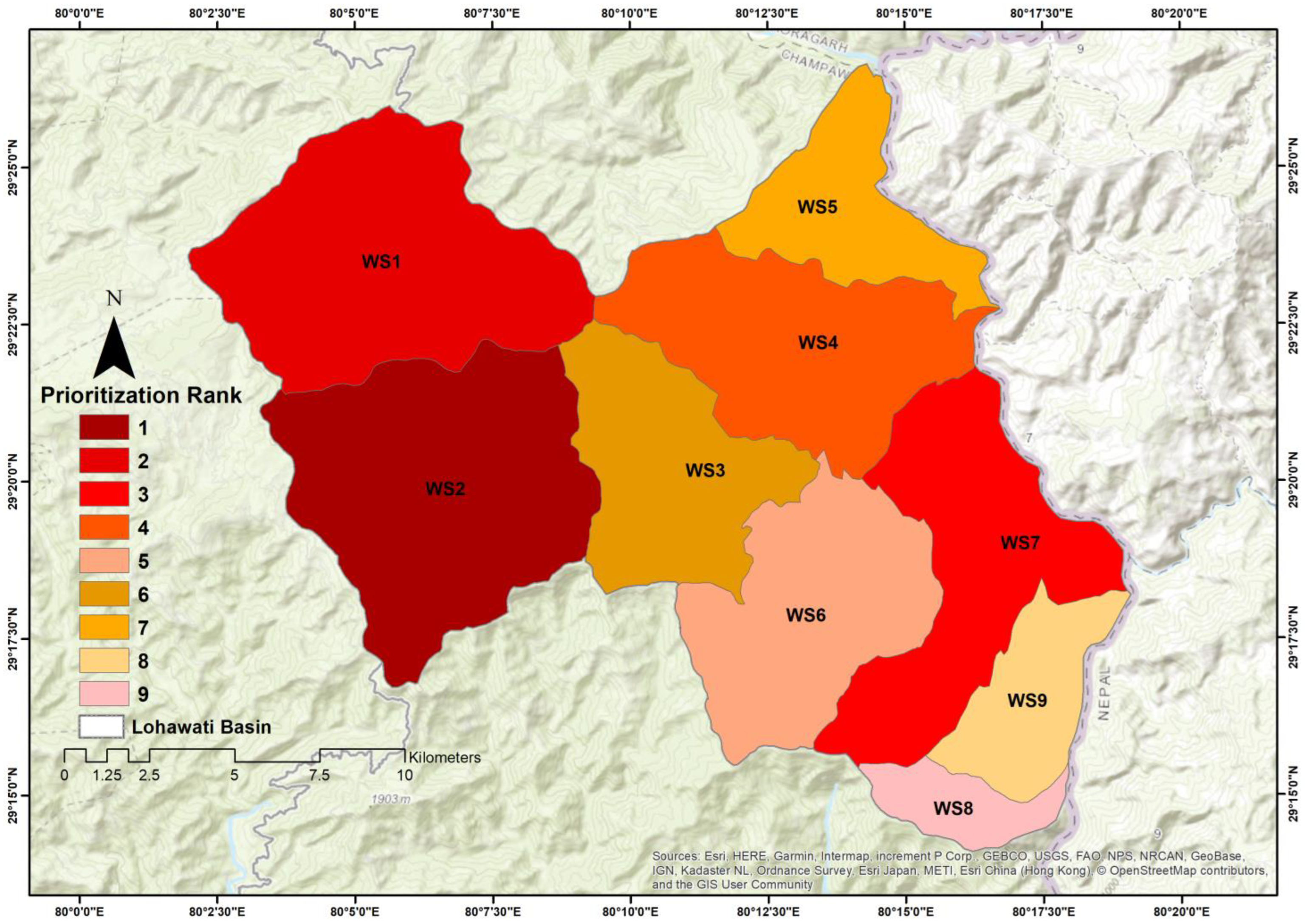
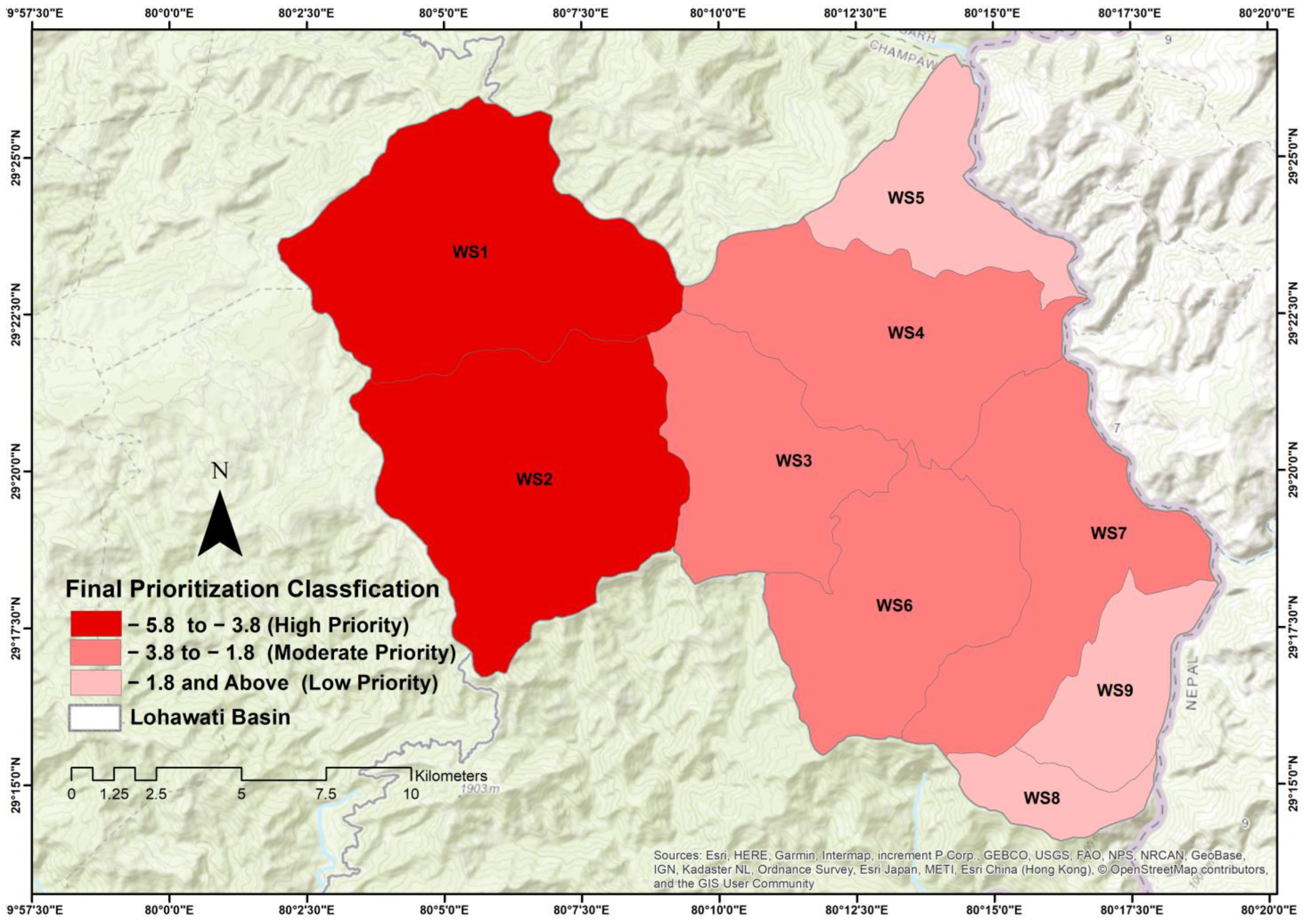
3.5. Prioritisation of the Watersheds

Watersheds exhibit diverse behaviour depending on their morphometric attributes, and identifying the critical watersheds is indispensable for cohesive planning and management. The present research has divided the Lohawati basin into nine sub-watersheds, which have been considered for prioritisation. The parameters; such as linear morphometric parameters, like mean bifurcation ratio and the length of overland flow; areal morphometric parameters, like basin area, form factor, elongation ratio, circularity ratio, shape factor, and shape index; texture parameters, like drainage density, drainage texture, texture ratio, and stream frequency; and relief morphometric parameters, like relief ratio and the ruggedness number have been taken into account for preliminary prioritisation ranking. Geomorphometric variables under linear, texture, and relief aspects are directly related to runoff and soil erosion, so a higher order was assigned to the parameters with higher values and vice versa. Similarly, variables under areal aspects are inversely related to runoff and soil erosion, so a higher ranking was given to the variable with a lower value and vice versa [49,55,97]. The ranking of morphometric variables considered for priority is shown in

Table 7. Initial prioritisation ranking of the watersheds in the Lohawati basin based on morphometric analysis.

Watershed	Basin Area	Elongation Ratio	Circulatory Ratio	Form Factor	Shape Index	Shape Factor	Stream Frequency	Drainage Density	Mean Bifurcation Ratio	Length of Overland Flow	Texture Ratio	Drainage Texture	Relief Ratio	Ruggedness Number
WS1	8	6	9	6	4	8	2	2	4	2	2	2	9	9
WS2	9	9	8	9	1	9	1	1	3	1	1	1	8	6
WS3	4	5	5	5	5	5	3	3	7	3	4	4	6	4
WS4	7	4	4	4	6	7	4	5	1	5	3	3	5	1
WS5	3	7	2	7	3	2	9	9	8	9	8	8	2	7
WS6	5	8	6	8	2	6	6	4	6	4	5	5	4	3
WS7	6	2	1	2	8	4	5	6	2	6	6	6	7	2
WS9	1	1	3	1	9	1	8	7	5	7	9	9	1	5

.

Once the erosion assessment parameters were evaluated and ranked, a correlation matrix was built using the WSA method (

Table 8. Correlation matrix representing the relationships between the morphometric properties of the watersheds.

	Basin Area	Elongation Ratio	Circulatory Ratio	Form Factor	Shape Index	Shape Factor	Stream Frequency	Drainage Density	Mean Bifurcation Ratio	Length of Overland Flow	Texture Ratio	Drainage Texture	Relief Ratio	Ruggedness Number
Basin area	1.000	0.533	0.433	0.533	−0.533	0.933	−0.850	−0.783	−0.700	−0.783	−0.917	−0.917	0.883	−0.117
Elongation ratio	0.533	1.000	0.500	1.000	−1.000	0.617	−0.383	−0.517	0.083	−0.517	−0.567	−0.567	0.350	0.217
Circulatory ratio	0.433	0.500	1.000	0.500	−0.500	0.667	−0.600	−0.650	0.100	−0.650	−0.650	−0.650	0.483	0.550
Form factor	0.533	1.000	0.500	1.000	−1.000	0.617	−0.383	−0.517	0.083	−0.517	−0.567	−0.567	0.350	0.217
Shape index	−0.533	−1.000	−0.500	−1.000	1.000	−0.617	0.383	0.517	−0.083	0.517	0.567	0.567	−0.350	−0.217
Shape factor	0.933	0.617	0.667	0.617	−0.617	1.000	−0.900	−0.883	−0.533	−0.883	−0.983	−0.983	0.833	−0.050
Stream frequency	−0.850	−0.383	−0.600	−0.383	0.383	−0.900	1.000	0.933	0.533	0.933	0.950	0.950	−0.917	0.033
Drainage density	−0.783	−0.517	−0.650	−0.517	0.517	−0.883	0.933	1.000	0.450	1.000	0.900	0.900	−0.817	0.033
Mean bifurcation ratio	−0.700	0.083	0.100	0.083	−0.083	−0.533	0.533	0.450	1.000	0.450	0.517	0.517	−0.533	0.550
Length of overland flow	−0.783	−0.517	−0.650	−0.517	0.517	−0.883	0.933	1.000	0.450	1.000	0.900	0.900	−0.817	0.033
Texture ratio	−0.917	−0.567	−0.650	−0.567	0.567	−0.983	0.950	0.900	0.517	0.900	1.000	1.000	−0.867	0.033
drainage texture	−0.917	−0.567	−0.650	−0.567	0.567	−0.983	0.950	0.900	0.517	0.900	1.000	1.000	−0.867	0.033
Relief ratio	0.883	0.350	0.483	0.350	−0.350	0.833	−0.917	−0.817	−0.533	−0.817	−0.867	−0.867	1.000	0.033
Ruggedness number	−0.117	0.217	0.550	0.217	−0.217	−0.050	0.033	0.033	0.550	0.033	0.033	0.033	0.033	1.000
Sum of correlations	−1.283	0.750	0.533	0.750	−0.750	−1.167	1.683	1.567	2.433	1.567	1.317	1.317	−1.233	2.350
Grand total	9.833	9.833	9.833	9.833	9.833	9.833	9.833	9.833	9.833	9.833	9.833	9.833	9.833	9.833
Prioritisation ranking	−0.131	0.076	0.054	0.076	−0.076	−0.119	0.171	0.159	0.247	0.159	0.134	0.134	−0.125	0.239

). The morphometric parameters were then assigned weights. It can be seen from Table 8 that most parameters, such as the basin area, form factor, elongation ratio, circularity ratio, shape factor, and shape index, showed a negative correlation with most of the other parameters. The matrix also showed that the form factor and elongation ratio, drainage density and length of overland flow, and drainage texture and texture ratios exhibited the highest positive correlation of one (1). The shape index and form factor and the shape index and elongation ratio showed the highest negative correlation of −1 (Table 8). The WSA method yielded a total of 9.833 from the sum of correlations. To determine the final weights for each parameter, the sum of the correlation coefficients of each parameter was divided by the total number of correlations. These weights were then assigned to the parameters in the prioritisation model to assess priority, as depicted in Equation (2).

Prioritization = (−0.131 × A) + (0.076 × Re) + (0.054 × Rc) + (0.076 × Ff) + (−0.076 × Si) + (−0.119 × Sf) + (0.171 × Fs) + (0.159 × Dd) + (0.247 × Rb) + (0.159 × Lg) + (0.134 × Rt) + (0.134 × Dt) + (−0.125 × Rh) + (0.239 × Rn)

(2)

The weights of each morphometric component were used to determine the prioritisation values for all the watersheds in the Lohawati basin (

Table 9. The process of prioritising and assigning the final ranking to the watersheds in the Lohawati basin.

S. No.	Code	Prioritisation Value	Rank
1.	WS1	−5.7876	2
2.	WS2	−5.8231	1
3.	WS3	−2.7221	6
4.	WS4	−3.4580	4
5.	WS5	−1.7420	7
6.	WS6	−3.4411	5
7.	WS7	−3.5703	3
8.	WS8	0.1646	9
8.	WS9	−1.0572	8

).

The prioritisation rating system ranked the hydrological units based on their prioritisation values, with the watershed having the smallest value being assigned top priority (one). The units were then ranked in ascending order of their values to determine their respective rankings. The WS2 received the highest priority ranking of one due to its lowest prioritisation value (−5.8231), WS1 was assigned second rank, with a prioritisation value of (−5.7876), and accordingly, the ranking was given to the other watersheds based on their corresponding prioritisation values (Table 9). The results suggest that WS2 is the most threatened watershed and is in immediate need of attention regarding soil, water, and vegetation resource management. Figure 8 displays the final map, indicating the priority ranking of the watersheds in the Lohawati basin. Further, the watersheds of the study area were categorised into high-, moderate-, and low-prioritisation zones based on the prioritisation values (Figure 9 and

Table 10. Grouping the sub-watersheds of the Lohawati basin based on their priority zones.

S. No.	Priority Zone	Priority Rank Range	Watershed Code	Area	Area (%)
1.	High	−5.8 to −3.8	WS1 and WS2	121.95 km2	36.14
2.	Moderate	−3.8 to −1.8	WS3, WS4, WS6, and WS7	164.91 km2	48.87
3.	Low	−1.8 and above	WS5, WS8, and WS9	50.62 km2	15.00

). As such, a 121.95 km² (36.14%) area of the basin is in a high-priority zone, 164.91 km² (48.87%) of the area is in the moderate-priority zone, and 50.62 km² (15%) of the area is in the low-prioritisation zone.

Identifying critical watersheds holds significant importance in natural resource management, especially to formulate watershed management strategies. This is because each watershed exhibits distinct hydrological behaviour based on its specific morphometric and topo-hydrological features [98,99]. Several watershed prioritisation methods are available, such as Principal Component Analysis, Multicriteria Decision Analysis, Sediment Yield Index, and Compound Factor [33,39,43,44,48,51,53,56,58,100]. In the past, sub-watershed prioritisation has predominantly relied on evaluating single categories of data, such as hydrology, land use, or soil texture, as observed in the aforementioned approaches [40]. However, this limited approach can overlook the complex interactions and interdependencies between various factors, potentially leading to suboptimal prioritisation outcomes.

Moreover, Multi-Criteria Decision Making (MCDM)-based approaches, which involve expert judgment, may face declining accuracy when confronted with new uncertainties [101,102]. This decrease in accuracy poses a challenge, especially in the absence of experts with in-depth knowledge of watershed dynamics [103]. On the other hand, sediment yield and erosion (SYE)-based methods demand specific soil erosion and sediment data [31], which might not be readily available in many countries. As a result, accurately estimating silt transport in watersheds with limited data has proven to be challenging [43], hindering the development of effective sediment yield management strategies.

To address these uncertainties and limitations, there is a pressing need to devise innovative methods to overcome these challenges and to provide valuable insights into the complex process of sediment yield in watershed management research [101]. One such effort to tackle these issues is the proposed Weighted Sum Analysis (WSA) model introduced by [40]. The WSA model offers a promising solution by incorporating multiple criteria and effectively dealing with uncertainties in data, thereby providing a more comprehensive and reliable approach to prioritise sub-watersheds.

By adopting the WSA model, researchers can consider the combined influence of various factors on watershed dynamics and prioritise sub-watersheds more accurately, even when faced with limited data availability or uncertainties for expert judgment. Developing and utilising such novel methods are essential for enhancing our understanding of sediment yield and improving watershed management strategies to ensure sustainable and effective conservation practices. Also, the data used are readily available for prioritisation studies. The approach introduced by [40] was employed for this study, and specific extra morphometric parameters were incorporated to improve the outcomes. The prioritisation ratings, obtained through the WSA technique, suggest that the morphometric characterisation tool serves as an efficient alternative to resource-intensive conventional soil and water risk assessment methods, mainly when data is limited or unavailable.

4. Conclusions

There are many different methods for performing river basin prioritisation, but some of them require a lot of data, some are arduous and time-consuming, and some are location-specific. In the current work, the morphometric variables and sub-watersheds of the Lohawati basin were extracted from ASTER satellite data, and a Weighted Sum Analysis (WSA) approach was used to prioritise the watersheds. The basic, shape, texture, and relief morphometric factors were estimated. The observed variation in the stream length ratio is attributed to the diverse slope gradients and topographic features present in the area. The varying slopes influence the flow patterns of streams, leading to different stream lengths across the basin.

Moreover, the lower drainage density (Dd) value of the Lohawati basin suggests the presence of impermeable rocks and moderate relief, creating favourable conditions for infiltration and enhancing groundwater prospects. This can have significant implications on overall water availability and sustainability in the region. The analysis of the watershed drainage texture revealed an extremely granular roughness, which further influences the flow paths and water movement within the basin. Additionally, the watershed relief indicated a mild to moderate slope, facilitating slow runoff and allowing for intense infiltration. These hydrological features can play a crucial role in regulating water flow, minimising the risk of flooding, and sustaining water resources in the Lohawati basin.

According to the risk of soil erosion, the watersheds in the Lohawati basin were ranked, with WS2 being the most susceptible and WS8 being the least susceptible. Additionally, watersheds were divided into high-, moderate-, and low-priority zones based on the prioritisation rank ranges. Because of the greater risk of runoff and soil erosion, the high-priority zones require urgent planning and the implementation of watershed management methods. As a result of combining geospatial and statistical methods, WSA has shown to be a substantial and valuable prioritisation approach, especially in data-deficient regions. The WSA method is a dynamic, efficient, and sustainable alternative to traditional prioritisation strategies that treat all characterisation parameters equally and in a complex manner. Decision makers, water resource managers, and conservation plan developers can all benefit from using the WSA method for sub-watershed prioritisation.

Nevertheless, given the ever-changing nature of hydrological systems, it would be advantageous to investigate how the WSA method adapts to varying environmental conditions and to evaluate its effectiveness over extended periods. Furthermore, integrating higher-resolution satellite images could be advantageous, leading to more promising outcomes for improved planning and management. Such investigations would offer valuable insights into the method’s durability and dependability amidst the continuous evolution of climate and land-use patterns.

References

1. Chopra, R.; Dhiman, R.D.; Sharma, P.K. Morphometric analysis of sub-watersheds in Gurdaspur district, Punjab using remote sensing and GIS techniques. J. Indian. Soc. Remote Sens. 2005, 33, 531–539. [Google Scholar] [CrossRef]
2. Ghosh, M.; Gope, D. Hydro-morphometric characterization and prioritization of sub-watersheds for land and water resource management using fuzzy analytical hierarchical process (FAHP): A case study of upper Rihand watershed of Chhattisgarh State, India. Appl. Water. Sci. 2021, 11, 1–20. [Google Scholar] [CrossRef]
3. Prabhakar, A.K.; Singh, K.K.; Lohani, A.K.; Chandniha, S.K. Study of Champua watershed for management of resources by using morphometric analysis and satellite imagery. Appl. Water. Sci. 2019, 9, 127. [Google Scholar] [CrossRef]
4. Raj, P.N.; Azeez, P.A. Morphometric analysis of a tropical medium river system: A case from Bharathapuzha River Southern India. Open. J. Modern. Hydrol. 2012, 2, 91–98. [Google Scholar]
5. Altaf, F.; Meraj, G.; Romshoo, S.A. Morphometric analysis to infer hydrological behaviour of Lidder watershed, Western Himalaya, India. Geog. J. 2013, 2013, 178021. [Google Scholar] [CrossRef]
6. Puno, G.R.; Puno, R.C.C. Watershed conservation prioritization using geomorphometric and land use-land cover parameters. Glob. J. Environ. Sci. Manag. 2019, 5, 279–294. [Google Scholar]
7. Jasmin, I.; Mallikarjuna, P. Morphometric analysis of Araniar river basin using remote sensing and geographical information system in the assessment of groundwater potential. Arab. J. Geosci. 2013, 6, 3683–3692. [Google Scholar] [CrossRef]
8. Horton, R.E. Drainage-basin characteristics. Trans. Am. Geophy. Union. 1932, 13, 350–361. [Google Scholar] [CrossRef]
9. Horton, R.E. An approach toward a physical interpretation of infiltration-capacity. Soil Sci. Soc. Am. J. 1941, 5, 399–417. [Google Scholar] [CrossRef]
10. Miller, V.C. Quantitative Geomorphic Study of Drainage Basin Characteristics in the Clinch Mountain area, Virginia and Tennessee; Technical Report; Columbia University: New York, NY, USA, 1953; pp. 389–402. [Google Scholar]
11. Schumm, S.A. Evolution of drainage systems and slopes in badlands at Perth Amboy, New Jersey. Geol. Soc. Am. Bull. 1956, 67, 597–646. [Google Scholar] [CrossRef]
12. Strahler, A. Statistical Analysis in Geomorphic Research. J. Geol. 1954, 62, 1. [Google Scholar] [CrossRef]
13. Strahler, A.N. Quantitative analysis of watershed geomorphology. Trans. Am. Geophy. Union. 1957, 38, 913–920. [Google Scholar] [CrossRef]
14. Strahler, A.N. Part II. Quantitative geomorphology of drainage basins and channel networks. In Handbook of Applied Hydrology; McGraw-Hill: New York, NY, USA, 1964; pp. 4–39. [Google Scholar]
15. Das, S.; Pardeshi, S.D. ; Pardeshi, S.D. Morphometric analysis of Vaitarna and Ulhas river basins, Maharashtra, India: Using geospatial techniques. Appl. Water. Sci. 2018, 8, 158. [Google Scholar] [CrossRef]
16. Ganie, P.A.; Posti, R.; Kumar, P.; Singh, A. Morphometric analysis of a Kosi River Basin, Uttarakhand using geographical information system. Int. J. Multidisc. Current Res. 2016, 4, 1190–1200. [Google Scholar]
17. Ganie, P.A.; Posti, R.; Aswal, A.S.; Bharti, V.S.; Sehgal, V.K.; Sarma, D.; Pandey, P.K. A comparative analysis of the vertical accuracy of multiple open-source digital elevation models for the mountainous terrain of the north-western Himalaya. Model. Earth Syst. Environ. 2023, 9, 2723–2743. [Google Scholar] [CrossRef]
18. Khatoon, T.; Javed, A. Morphometric Behavior of Shahzad Watershed, Lalitpur District, Uttar Pradesh, India: A Geospatial Approach. J. Geogr. Inf Syst. 2022, 14, 193–220. [Google Scholar] [CrossRef]
19. Kumar, L.; Joshi, G.; Agarwal, K.K. Morphometry and Morphostructural Studies of the Parts of Gola River and Kalsa River Basins, Chanphi-Okhalkanda Region, Kumaun Lesser Himalaya, India. Geotectonics. 2020, 54, 410–427. [Google Scholar] [CrossRef]
20. Mangan, P.; Haq, M.A.; Baral, P. Morphometric analysis of watershed using remote sensing and GIS—A case study of Nanganji River Basin in Tamil Nadu, India. Arab. J. Geosci. 2019, 12, 202. [Google Scholar] [CrossRef]
21. Manjare, B.S.; Padhye, M.A.; Girhe, S.S. Morphometric analysis of a Lower Wardha River sub basin of Maharashtra, India Using ASTER DEM Data and GIS. Proceedings of Geo-Enabling Digital India, 15th ESRI India User Conference, New Delhi, India, 9–11 December 2014; pp. 1–13. [Google Scholar]
22. Muhtadi, A.; Aldiano, R.; Leidonald, R. Morphometric characteristics of the Alas-Singkil drainage basins. In IOP Conference Series: Earth and Environmental Science; IOP Publishing: Bristol, UK, 2022; Volume 977, p. 012090. [Google Scholar]
23. Soni, S. Assessment of morphometric characteristics of Chakrar watershed in Madhya Pradesh India using geospatial technique. Appl. Water. Sci. 2017, 7, 2089–2102. [Google Scholar] [CrossRef]
24. Tassew, B.G.; Belete, M.A.; Miegel, K. Assessment and analysis of morphometric characteristics of Lake Tana sub-basin, Upper Blue Nile Basin, Ethiopia. Int. J. River Basin. Manag. 2021, 21, 195–209. [Google Scholar] [CrossRef]
25. Umrikar, B.N. Morphometric analysis of Andhale watershed, Taluka Mulshi, District Pune, India. Appl. Water. Sci. 2017, 7, 2231–2243. [Google Scholar] [CrossRef]
26. Moore, I.D.; Grayson, R.B.; Ladson, A.R. Digital terrain modelling: A review of hydrological, geomorphological, and biological applications. Hydrol. Process. 1991, 5, 3–30. [Google Scholar] [CrossRef]
27. Bajirao, T.S.; Kumar, P.K.; Kumar, P.K.; Tarate, C.; Bajirao, S. Application of remote sensing and GIS for morphometric analysis of watershed: A Review. Int. J. Chem. Stud. 2019, 7, 709–713. [Google Scholar]
28. Choudhari, P.P.; Nigam, G.K.; Singh, S.K.; Thakur, S. Morphometric based prioritization of watershed for groundwater potential of Mula river basin, Maharashtra, India. Geol. Ecol. Landscapes 2018, 2, 256–267. [Google Scholar] [CrossRef]
29. Khurana, D.; Rawat, S.S.; Raina, G.; Sharma, R.; Jose, P.G. GIS-Based Morphometric Analysis and Prioritization of Upper Ravi Catchment, Himachal Pradesh, India. In Advances in Water Resources Engineering and Management; Springer: Singapore, 2019; pp. 163–185. [Google Scholar] [CrossRef]
30. Harsha, J.; Ravikumar, A.S.; Shivakumar, B.L. Evaluation of morphometric parameters and hypsometric curve of Arkavathy river basin using RS and GIS techniques. Appl. Water Sci. 2020, 10, 86. [Google Scholar] [CrossRef]
31. Shivhare, N.; Rahul, A.K.; Omar, P.J.; Chauhan, M.S.; Gaur, S.; Dikshit, P.K.S.; Dwivedi, S.B. Identification of critical soil erosion prone areas and prioritization of micro-watersheds using geoinformatics techniques. Ecol. Eng. 2018, 121, 26–34. [Google Scholar] [CrossRef]
32. Pandey, A.; Chowdary, V.M.; Mal, B.C. Identification of critical erosion prone areas in the small agricultural watershed using USLE, GIS and remote sensing. Water Resour. Manag. 2006, 21, 729–746. [Google Scholar] [CrossRef]
33. Arabameri, A.; Pradhan, B.; Pourghasemi, H.R.; Rezaei, K. Identification of erosion-prone areas using different multi-criteria decision-making techniques and GIS. Geomat. Nat. Hazards Risk 2018, 9, 1129–1155. [Google Scholar] [CrossRef]
34. Jain, P.; Ramsankaran, R. GIS-based integrated multi-criteria modelling framework for watershed prioritisation in India—A demonstration in Marol watershed. J. Hydrol. 2019, 578, 124131. [Google Scholar] [CrossRef]
35. Jaiswal, R.; Ghosh, N.; Galkate, R.; Thomas, T. Multi Criteria Decision Analysis (MCDA) for Watershed Prioritization. Aquat. Procedia 2015, 4, 1553–1560. [Google Scholar] [CrossRef]
36. Rahaman, S.A.; Ajeez, S.A.; Aruchamy, S.; Jegankumar, R. Prioritization of Sub Watershed Based on Morphometric Characteristics Using Fuzzy Analytical Hierarchy Process and Geographical Information System—A Study of Kallar Watershed, Tamil Nadu. Aquat. Procedia 2015, 4, 1322–1330. [Google Scholar] [CrossRef]
37. Rahmati, O.; Haghizadeh, A.; Stefanidis, S. Assessing the Accuracy of GIS-Based Analytical Hierarchy Process for Watershed Prioritization; Gorganrood River Basin, Iran. Water Resour. Manag. 2015, 30, 1131–1150. [Google Scholar] [CrossRef]
38. Shivhare, V.; Gupta, C.; Mallick, J.; Singh, C.K. Geospatial modelling for sub-watershed prioritization in Western Himalayan Basin using morphometric parameters. Nat. Hazards 2021, 110, 545–561. [Google Scholar] [CrossRef]
39. Toosi, S.R.; Samani, J.M.V. Prioritizing watersheds using a novel hybrid decision model based on fuzzy DEMATEL, fuzzy ANP and fuzzy VIKOR. Water Resour. Manag. 2017, 31, 2853–2867. [Google Scholar] [CrossRef]
40. Aher, P.; Adinarayana, J.; Gorantiwar, S. Quantification of morphometric characterization and prioritization for management planning in semi-arid tropics of India: A remote sensing and GIS approach. J. Hydrol. 2014, 511, 850–860. [Google Scholar] [CrossRef]
41. Kadam, A.K.; Jaweed, T.H.; Kale, S.S.; Umrikar, B.N.; Sankhua, R.N. Identification of erosion-prone areas using modified morphometric prioritization method and sediment production rate: A remote sensing and GIS approach. Geomat. Nat. Hazards Risk 2019, 10, 986–1006. [Google Scholar] [CrossRef]
42. Malik, A.; Kumar, A.; Kandpal, H. Morphometric analysis and prioritization of sub-watersheds in a hilly watershed using weighted sum approach. Arab. J. Geosci. 2019, 12, 118. [Google Scholar] [CrossRef]
43. Ayele, G.T.; Teshale, E.Z.; Yu, B.; Rutherfurd, I.D.; Jeong, J. Streamflow and Sediment Yield Prediction for Watershed Prioritization in the Upper Blue Nile River Basin, Ethiopia. Water 2017, 9, 782. [Google Scholar] [CrossRef]
44. Bali, Y.P.; Karale, R.L. Sediment Yield Index as a Criterion for Choosing Priority Basins; IAHS-AISH Publication: Paris, France, 1977; pp. 180–188. [Google Scholar]
45. Chakraborti, A.K. Sediment yield prediction and prioritization of watershed using remote sensing data. In Proceedings of the 12th Asian Conference on Remote Sensing, Singapore, 30 October–5 November 1991. [Google Scholar]
46. Gajbhiye, S.; Sharma, S.K.; Meshram, C. Prioritization of Watershed through Sediment Yield Index Using RS and GIS Approach. Int. J. u- and e-Serv. Sci. Technol. 2014, 7, 47–60. [Google Scholar] [CrossRef]
47. Kumar, K.A.; Sandeep, P.; Masilamani, P. Prioritization of Watershed using Sediment Yield Index Method: A Case study of Semi-Arid Ecosystem of South India. Environ. We Int. J. Sci. Tech. 2021, 16, 1–13. [Google Scholar]
48. Naqvi, H.R.; Athick, A.M.A.; Ganaie, H.A.; Siddiqui, M.A. Soil erosion planning using sediment yield index method in the Nun Nadi watershed, India. Int. Soil Water Conserv. Res. 2015, 3, 86–96. [Google Scholar] [CrossRef]
49. Rajasekhar, M.; Raju, G.S.; Raju, R.S. Morphometric analysis of the Jilledubanderu River Basin, Anantapur District, Andhra Pradesh, India, using geospatial technologies. Groundw. Sustain. Dev. 2020, 11, 100434. [Google Scholar] [CrossRef]
50. Ratnam, K.N.; Srivastava, Y.K.; Rao, V.V.; Amminedu, E.; Murthy, K.S.R. Check dam positioning by prioritization of micro-watersheds using SYI model and morphometric analysis—Remote sensing and GIS perspective. J. Indian Soc. Remote Sens. 2005, 33, 25–38. [Google Scholar] [CrossRef]
51. Samal, D.R.; Gedam, S.S.; Nagarajan, R. GIS based drainage morphometry and its influence on hydrology in parts of Western Ghats region, Maharashtra, India. Geocarto Int. 2015, 30, 755–778. [Google Scholar] [CrossRef]
52. Ayadi, I.; Abida, H.; Djebbar, Y.; Mahjoub, M.R. Sediment yield variability in central Tunisia: A quantitative analysis of its controlling factors. Hydrol. Sci. J.-J. Des Sci. Hydrol. 2010, 55, 446–458. [Google Scholar] [CrossRef]
53. Meshram, S.G.; Sharma, S.K. Prioritization of watershed through morphometric parameters: A PCA-based approach. Appl. Water Sci. 2015, 7, 1505–1519. [Google Scholar] [CrossRef]
54. Sharma, S.K.; Tignath, S.; Gajbhiye, S.; Patil, R. Application of principal component analysis in grouping geomorphic parameters of Uttela watershed for hydrological modeling. Int. J. Remote Sens. Geosci. 2013, 2, 63–70. [Google Scholar]
55. Bharath, A.; Kumar, K.K.; Maddamsetty, R.; Manjunatha, M.; Tangadagi, R.B.; Preethi, S. Drainage morphometry based sub-watershed prioritization of Kalinadi basin using geospatial technology. Environ. Chall. 2021, 5, 100277. [Google Scholar] [CrossRef]
56. Farhan, Y.; Anaba, O. A Remote Sensing and GIS Approach for Prioritization of Wadi Shueib Mini-Watersheds (Central Jordan) Based on Morphometric and Soil Erosion Susceptibility Analysis. J. Geogr. Inf. Syst. 2016, 8, 1–19. [Google Scholar] [CrossRef]
57. Gajbhiye, S.; Mishra, S.K.; Pandey, A. Prioritizing erosion-prone area through morphometric analysis: An RS and GIS perspective. Appl. Water Sci. 2013, 4, 51–61. [Google Scholar] [CrossRef]
58. Mallick, J.; Shivhare, V.; Singh, C.K.; Al Subih, M. Prioritizing Watershed Restoration, Management, and Development Based on Geo-Morphometric Analysis in Asir Region of Saudi Arabia Using Geospatial Technology. Pol. J. Environ. Stud. 2022, 31, 1201–1222. [Google Scholar] [CrossRef] [PubMed]
59. Valdiya, K.S. Geology of Kumaun Lesser Himalaya; Wadia Institute of Himalayan Geology: Dehradun, India, 1980; 291p. [Google Scholar]
60. Valdiya, K.S. An outline of the structural set-up of Kumaun Himalaya. J. Geol. Soc. India 1979, 20, 145–157. [Google Scholar]
61. IMD Indian Meteorological Department. 2022. Available online: https://mausam.imd.gov.in (accessed on 25 September 2022).
62. Abrams, M.; Hook, S.; Ramachandran, B. ASTER User Handbook Version 2; Jet Propulsion Laboratory: Pasadena, CA, USA, 2002; Volume 2003. [Google Scholar]
63. Ahmed, S.A.; Chandrashekarappa, K.N.; Raj, S.K.; Nischitha, V.; Kavitha, G. Evaluation of morphometric parameters derived from ASTER and SRTM DEM—A study on Bandihole sub-watershed basin in Karnataka. J. Indian Soc. Remote Sens. 2010, 38, 227–238. [Google Scholar] [CrossRef]
64. Tarboton, D.G.; Bras, R.L.; Rodriguez-Iturbe, I. On the extraction of channel networks from digital elevation data. Hydrol. Process. 1991, 5, 81–100. [Google Scholar] [CrossRef]
65. Horton, R.E. Erosional development of streams and their drainage basins: Hydrophysical approach to quantitative morphology. Bull. Geol. Soc. Am. 1945, 56, 275–370. [Google Scholar] [CrossRef]
66. Sameena, M.; Krishnamurthy, J.; Jayaraman, V.; Ranganna, G. Evaluation of drainage networks developed in hard rock ter-rain. Geocarto Int. 2009, 24, 397–420. [Google Scholar] [CrossRef]
67. Faniran, A. The index of drainage intensity: A provisional new drainage factor. Austr. J. Sci. 1968, 31, 326–330. [Google Scholar]
68. Bhat, S.; Romshoo, S. Digital elevation model based watershed characteristics of upper watersheds of Jhelum basin. J. Appl. Hydro. 2009, 21, 23–34. [Google Scholar]
69. Amiri, M.; Pourghasemi, H.R.; Arabameri, A.; Vazirzadeh, A.; Yousefi, H.; Kafaei, S. Prioritization of flood inundation of Ma-harloo Watershed in iran using morphometric parameters analysis and TOPSIS MCDM model. In Spatial Modeling in GIS and R for Earth and Environmental Sciences; Elsevier: Amsterdam, The Netherlands, 2019; pp. 371–390. [Google Scholar]
70. Magesh, N.S.; Chandrasekar, N. GIS model-based morphometric evaluation of Tamiraparani subbasin, Tirunelveli district, Tamil Nadu, India. Arab. J. Geosci. 2012, 7, 131–141. [Google Scholar] [CrossRef]
71. Costa, J.E. Hydraulics and basin morphometry of the largest flash floods in the conterminous United States. J. Hydrol. 1987, 93, 313–338. [Google Scholar] [CrossRef]
72. Sreedevi, P.D.; Owais, S.H.H.K.; Khan, H.H.; Ahmed, S. Morphometric analysis of a watershed of South India using SRTM data and GIS. J. Geol. Soc. India. 2009, 73, 543–552. [Google Scholar] [CrossRef]
73. Gregory, K.J.; Walling, D.E. Drainage Basin form and Process a Geomorphological Approach; Edward Arnold: London, UK, 1973; p. 456. [Google Scholar]
74. Dar, R.A.; Chandra, R.; Romshoo, S.A. Morphotectonic and lithostratigraphic analysis of intermontane Karewa Basin of Kashmir Himalayas, India. J. Mt. Sci. 2013, 10, 1–15. [Google Scholar] [CrossRef]
75. Reddy, G.P.O.; Maji, A.K.; Gajbhiye, K.S. Drainage morphometry and its influence on landform characteristics in a basaltic terrain, Central India—A remote sensing and GIS approach. Int. J. Appl. Earth Obs. Geoinf. 2004, 6, 1–16. [Google Scholar] [CrossRef]
76. Yangchan, J.; Jain, A.K.; Tiwari, A.K.; Sood, A. Morphometric analysis of drainage basin through GIS: A case study of Sukhna Lake Watershed in Lower Shiwalik, India. Int. J. Sci. Eng. Res. 2015, 6, 1015–1023. [Google Scholar] [CrossRef]
77. Vinutha, D.N.; Janardhana, M.R. Morphometry of The Payaswini Watershed, Coorg District, Karnataka, India, Using Remote Sensing and GIS. Techniques. Int. J. Innov. Res. Sci. Eng. Technol. 2014, 3, 516–524. [Google Scholar]
78. Bull, W.B.; McFadden, L.D. Tectonic Geomorphology North and South of the Garlock Fault, California. In Geomorphology in Arid Regions: Proceedings of the Eighth Annual Geomorphology Symposium, State University of New York at Binghamton, Binghamton, NY, USA, 23–24 September 1977; Doehring, D.O., Ed.; George Allen & Unwin Ltd.: Crows Nest, Australia, 1977; pp. 115–138. [Google Scholar]
79. Zaz, S.N.; Romshoo, S.A. Assessing the geoindicators of land degradation in the Kashmir Himalayan region, India. Nat. Hazards 2012, 64, 1219–1245. [Google Scholar] [CrossRef]
80. Suresh, M.; Sudhakar, S.; Tiwari, K.N.; Chowdary, V.M. Prioritization of watersheds using morphometric parameters and assessment of surface water potential using remote sensing. J. Indian Soc. Remote Sens. 2004, 32, 249–259. [Google Scholar] [CrossRef]
81. Melton, M.A. Geometric Properties of Mature Drainage Systems and Their Representation in an E4Phase Space. J. Geol. 1958, 66, 35–54. [Google Scholar] [CrossRef]
82. Das, A.K.; Mukherjee, S. Drainage morphometry using satellite data and GIS in Raigad district, Maharashtra. J. Geol. Soc. India 2005, 65, 577–586. [Google Scholar]
83. Ganie, P.A.; Posti, R.; Kunal, K.; Kunal, G.; Sarma, D.; Pandey, P.K. Insights into the morphometric characteristics of the Himalayan River using remote sensing and GIS techniques: A case study of Saryu basin, Uttarakhand, India. Appl. Geomat. 2022, 14, 707–730. [Google Scholar] [CrossRef]
84. Mesa, L.M. Morphometric analysis of a subtropical Andean basin (Tucumán, Argentina). Environ. Geol. 2006, 50, 1235–1242. [Google Scholar] [CrossRef]
85. Chorley, R.J. The drainage basin as the fundamental geomorphic unit. In Water, Earth and Man; Chorley, R.J., Ed.; Methuen: London, UK, 1969; pp. 77–98. [Google Scholar]
86. Chow, V.T.; Maidment, D.; Mays, L.W. Applied Hydrology; McGraw-Hill: New York, NY, USA, 1988. [Google Scholar]
87. Altın, T.B.; Altın, B.N. Drainage morphometry and its influence on landforms in volcanic terrain, Central Anatolia, Turkey. Procedia-Soc. Behav. Sci. 2011, 19, 732–740. [Google Scholar] [CrossRef]
88. Angillieri, M.Y.E. Morphometric analysis of Colangüil river basin and flash flood hazard, San Juan, Argentina. Environ. Geol. 2007, 55, 107–111. [Google Scholar] [CrossRef]
89. Potter, K.W.; Faulkner, E.B. Catchment response time as a predictor of flood quantiles. J. Am. Water Resour. Assoc. 1987, 23, 857–861. [Google Scholar] [CrossRef]
90. Hadley, R.F.; Schumm, S.A. Sediment Sources and Drainage Basin Characteristics in Upper Cheyenne River Basin; USGS water supply paper-1531 B; Scientific Research: Washington, DC, USA, 1961; p. 198. [Google Scholar]
91. Ahnert, F. Functional relationships between denudation, relief, and uplift in large, mid-latitude drainage basins. Am. J. Sci. 1970, 268, 243–263. [Google Scholar] [CrossRef]
92. Mustak, S.K.; Baghmar, N.K.; Ratre, C.R. Measurement of Dissection Index of Pairi River Basin Using Remote Sensing and GIS. Natl. Geogr. J. India 2012, 58, 97–106. [Google Scholar]
93. Gottschalk, L.C. Reservoir Sedimentation. In Handbook of Applied Hydrology; McGraw-Hill: New York, NY, USA, 1964. [Google Scholar]
94. Vijith, H.; Satheesh, R. GIS based morphometric analysis of two major upland sub-watersheds of meenachil river in Kerala. J. Indian Soc. Remote Sens. 2006, 34, 181–185. [Google Scholar] [CrossRef]
95. Selvan, M.T.; Ahmad, S.; Rashid, S.M. Analysis of the geomorphometric parameters in high altitude glacierized terrain using SRTM DEM data in Central Himalaya, India. ARPN J. Sci. Technol. 2011, 1, 22–27. [Google Scholar]
96. Patton, P.C. Drainage basin morphometry and floods. In Flood Geomorphology; John Wiley & Sons: New York, NY, USA, 1988; pp. 51–64. [Google Scholar]
97. Singh, W.R.; Barman, S.; Tirkey, G. Morphometric analysis and watershed prioritization in relation to soil erosion in Dudhnai Watershed. Appl. Water Sci. 2021, 11, 151. [Google Scholar] [CrossRef]
98. Jain, M.K.; Das, D. Estimation of Sediment Yield and Areas of Soil Erosion and Deposition for Watershed Prioritization using GIS and Remote Sensing. Water Resour. Manag. 2009, 24, 2091–2112. [Google Scholar] [CrossRef]
99. Javed, A.; Khanday, M.Y.; Rais, S. Watershed prioritization using morphometric and land use/land cover parameters: A remote sensing and GIS based approach. J. Geol. Soc. India 2011, 78, 63–75. [Google Scholar] [CrossRef]
100. Ganie, P.A.; Posti, R.; Kunal, K.; Kunal, G.; Bharti, V.S.; Sehgal, V.K.; Sarma, D.; Pandey, P.K. Modelling of the Himalayan Mountain river basin through hydro-morphological and compound factor-based approaches using geoinformatics tools. Model. Earth Syst. Environ. 2023, 9, 3053–3084. [Google Scholar] [CrossRef]
101. Adhami, M.; Sadeghi, S.H. Sub-watershed prioritization based on sediment yield using game theory. J. Hydrol. 2016, 541, 977–987. [Google Scholar] [CrossRef]
102. Balasubramanian, A.; Duraisamy, K.; Thirumalaisamy, S.; Krishnaraj, S.; Yatheendradasan, R.K. Prioritization of subwatersheds based on quantitative morphometric analysis in lower Bhavani basin, Tamil Nadu, India using DEM and GIS techniques. Arab. J. Geosci. 2017, 10, 552. [Google Scholar] [CrossRef]
103. Kruse, R.; Schwecke, E.; Heinsohn, J. Uncertainty and Vagueness in Knowledge Based Systems: Numerical Methods; Springer Science & Business Media: Berlin/Heidelberg, Germany, 2012. [Google Scholar]
Figure 1. (a) Location map of the study area indicating the location of the Uttarakhand and the positioning of the Lohawati basin. (b) Field photographs showcasing different sections of the Lohawati basin.
Conservation 03 00031 g001aConservation 03 00031 g001b
Figure 2. (a) ASTER data used for the study with Lohawati basin highlighted. (b) Lohawati basin.
Conservation 03 00031 g002
Figure 3. Extraction of drainage network of Lohawati basin.
Conservation 03 00031 g003
Figure 4. The flowchart outlining the methodology used to prioritise the watersheds of the Lohawati basin using the Weighted Sum Analysis approach.
Conservation 03 00031 g004
Figure 5. The drainage pattern of Lohawati basin.
Conservation 03 00031 g005
Figure 6. Watershed maps of the Lohawati basin.
Conservation 03 00031 g006aConservation 03 00031 g006bConservation 03 00031 g006c
Figure 7. Relief of the Lohawati basin.
Conservation 03 00031 g007
Figure 8. Sub-watershed prioritisation ranking map based on WSA values of the Lohawati basin.
Conservation 03 00031 g008
Figure 9. The priority-wise classification of the sub-watersheds of the Lohawati basin.
Conservation 03 00031 g009