Phytoplankton Community in Relation to Environmental Variables in the Tidal Mangrove Creeks of the Pasur River Estuary, Bangladesh

Abstract

The Pasur River estuary (PRE) provides vital fishery resources and supports millions of livelihoods in the southwestern coastal region of Bangladesh. Our research focused on phytoplankton community assemblages, alpha diversity indices, and the seasonal succession of major phytoplankton species in relation to physicochemical parameters in the tidal mangrove creeks of the Pasur River estuary. Spatial and temporal variations were assessed by water sampling at 17 stations in the study area from January to December 2019. The mean salinity level in the tidal mangrove creeks of the PRE was significantly (p < 0.05) higher during the dry season than during the wet season. Spatially, no significant variation (p > 0.05) was observed in the dissolved inorganic nitrogen and dissolved inorganic phosphorus between PRE and mangrove creeks, but temporally, the variables varied significantly (p < 0.05). Spatially, no significant variation (p > 0.05) was observed in the alpha diversity of the phytoplankton community but significantly (p < 0.05) varied temporally. Blue-green algae became dominant in the oligohaline conditions during the wet season, while diatoms were dominant during the dry season which severely depleted dissolved silica. In terms of phytoplankton species diversity, our study classifies the study areas as highly diversified zones. Phytoplankton succession from diatoms (dry season) to blue-green algae (wet season) is attributed to the changes in the physicochemical and nutrient parameters depending on seasonal environmental parameter fluctuations. This study illustrated that phytoplankton diversity and density varied with the degrees of habitat and seasonal changes, implying the potential impacts of anthropogenic activities and natural causes on their community structure in tropical estuaries and mangrove creeks.

1. Introduction

Estuaries are semi-enclosed coastal bodies of water having a free connection with the open sea [1] within which seawater is measurably diluted with fresh water derived from land drainage [1]. The world’s tropical and subtropical tidal mangrove estuaries and creeks are home to a wide variety of phytoplankton species [2]. Tropical tidal currents and estuarine ecosystems are fascinating in this regard because of their frequently changing hydrological conditions for studying phytoplankton dynamics [3]. In aquatic ecosystems, phytoplankton are the primary producers, while heterotrophic bacteria are the primary secondary producers [4,5]. Each species of phytoplankton has different habitat requirements that are favorable to reproduction, and the associated physicochemical parameters of estuarine ecosystems always influence the composition, abundance, and distribution of phytoplankton, resulting in a significant spatial and temporal change in the composition of the community [6].

Changes in the physicochemical conditions in the estuarine water affect the phytoplankton communities due to their short life cycle [7,8]. In addition, the season also influences the variation in physicochemical parameters that influence the structure and diversity of an estuary’s phytoplankton community [9,10]. Phytoplankton growth in estuarine water ultimately depends upon a seasonal and inter-annual climatological cycle that determines the availability of nutrients and light [11,12,13]. Increasing primary production and nutrient dynamics has an inevitable effect on the taxonomic composition of the phytoplankton community structure [14,15]. A combination of physical, chemical, and biological variables can control the seasonal succession of primary producers [15].

Some microalgae species, including diatoms and blue-green algae, have been identified as potentially toxic not only to aquatic life but also to human life [14]. Diatoms are dominant in marine and estuarine waters as a lifeform of phytoplankton and are used as a valuable indicator of the aquatic environment [5]. Responses of the phytoplankton community to seasonal changes will play a critical role in shaping phytoplankton communities in aquatic ecosystems. Alterations in monsoonal patterns, rainfall intensity, water currents, tidal changes, waves and outwelling will affect all factors related to photosynthesis, growth, composition and diversity of phytoplankton [5].

During the wet season, high rainfall and increased surface runoff caused an increase in the water turbidity and a decrease in water transparency, resulting in a reduction in light intensity and diatom density. It was noted that suspended sediments reduced light penetration and caused a decline in diatom growth. However, some species of green algae and blue-green algae respond positively to high turbidity as they have exceptional shade adaptation [5,15]. In terms of nutrient dynamics, tidal mangrove creeks and estuarine ecosystems are highly dynamic and productive areas with rich biodiversity [16,17]. The regular and periodic seasonal changes in physicochemical parameters (temperature, salinity, and nutrients), as well as hydrological variations such as tides, have a strong influence on estuarine life, which has a direct or indirect influence on phytoplankton community and structure [14].

The Pasur River estuary (PRE) is the largest estuary for the Sundarbans mangrove environment, located on Bangladesh’s southwestern coast [18]. Information about phytoplankton with respect to environmental variables in the PRE is limited [19,20,21,22,23,24]. In addition, studies on phytoplankton from the tidal mangrove creeks are scarce [25]. However, none of these studies showed that seasonal phytoplankton succession and alpha diversity indices in hydrologically connected aquatic habits of the PRE and the tidal mangrove creeks have not been documented. Hence, the present study was undertaken to analyze the phytoplankton community assemblage, phytoplankton alpha diversity indices, and the seasonal succession of major phytoplankton species related to physicochemical parameters in the tidal mangrove creeks of the PRE.

2. Materials and Methods

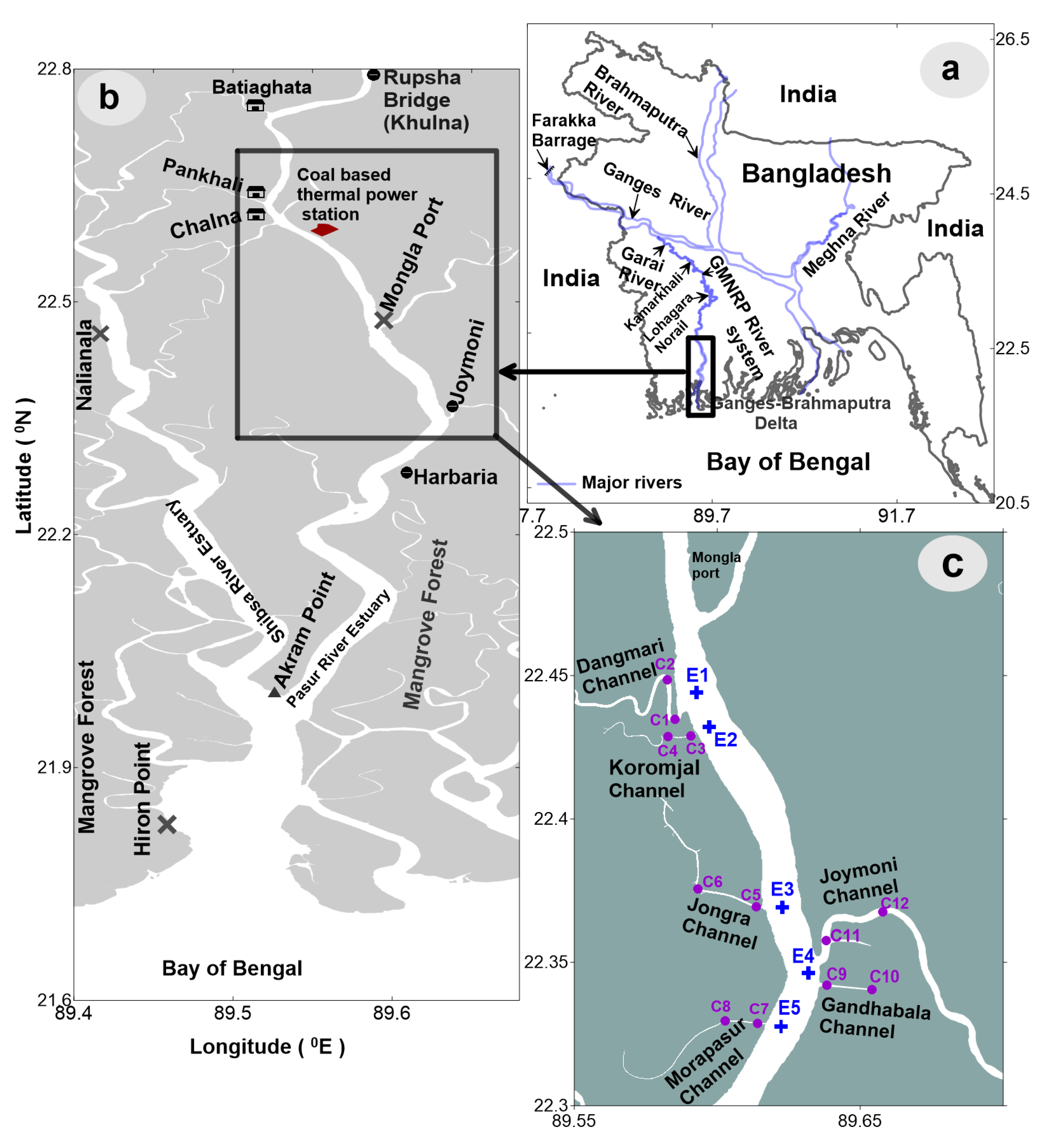
2.1. Study Area

The Pasur River estuary (PRE) is one of the most important estuaries that originated from the Gorai Madhumati Rupsha Pasur River System (GMRP). It is the main source of fresh water upstream of the Bay of Bengal, located in the southwestern coastal region of Bangladesh in the Sundarban [21,26], the world’s largest mangrove ecosystem. The PRE is connected by the Pankhali, Chunkhuri, and Batiaghata Channels to the Shibsa River estuary (SRE). The PRE is considered to have high primary productivity due to dissolved inorganic nutrients enrichment from mangroves through tidal creeks and therefore offers ideal fishing grounds [21]. The Sundarbans cover about 10,000 km² in the southwest of Bangladesh and West Bengal in India. The study area (Figure 1) comprises 17 sampling stations, including 12 stations located in the mangrove creeks (Dangmari channel: C1, C2; Koromjal channel: C3, C4; Jongra channel: C5, C6; Morapasur channel: C7, C8; Gandhabala channel: C9, C10; and Joymoni channel: C11, C12) and 5 stations in the main Pasur River estuary (E1, E2, E3, E4 and E5). The study areas were selected according to their geographical location.

2.2. Sample Collection and Laboratory Analysis

Water samples were collected on seven occasions from January 2019 to December 2019 to include both the dry (28 January 2019, 13 March 2019, 25 April 2019, 23 June 2019 and 31 December 2019) and wet seasons (24 August 2019 and 24 October 2019). Sampling dates were based on the Bangladesh Inland Water Transport Authority. At each sampling station, geographic coordinates were determined using a Garmin Etrex GPS. Surface water was sampled within a depth of 0–0.5 m (euphotic layer) in all seventeen stations using a 1.5 L water sampler (Wildco-1520) for nutrients analysis and environmental parameter determination, immediately filtered through Whatman GF/F (0.45) filter paper using a vacuum machine and refrigerated under dark conditions until laboratory analysis. After calibration, a DO meter (HACH HQ30d) was used to measure dissolved oxygen (DO) concentrations (calibration procedure: connect the probe to the meter, fill the provided plastic bottle with room temperature tap water, shake vigorously for 30 s, turn the meter on (probe must be connected before meter is on), remove the probe safety guard, then place the probe into the bottle, push the CALIBRATE key, and press the green button to activate calibration, select READ). As the probe stabilizes, the display will show Stabilizing and a progress bar. Select Done to view the calibration summary and Store to accept the calibration) and pH determined by a pH meter (sensION⁺ EC71) after calibration (calibration procedure: calibration is very important for highly accurate readings. The equipment is capable of calibration using 147 S/cm, 1413 S/cm, and 12.88 mS/cm standards, respectively. Nutrient analysis, including estimation of nitrite, nitrate, ammonia, inorganic phosphate, and silica, was carried out in the laboratory [27,28] and the values were determined by a spectrophotometric method (HACH, DR-6000, Germany, S/N: 1824775). Nitrite was analyzed by the USEPA diazotization method, ammonia was analyzed by the USEPA Nessler method, and phosphorus was analyzed by the USEPA Ascorbic acid method. Nitrate was analyzed by the HACH cadmium reduction method, and silica was analyzed by the HACH Heteropoly blue method. A vertical salinity and temperature profile were taken using a conductivity-temperature-depth (CTD) profiler (Model: In-situ Aqua TROLL 200, In-situ Inc., Lincoln Ave, Fort Collins, CO, USA) along the main axis of the PRE and the connecting mangrove creeks. Chlorophyll a analysis followed using the method based on Parsons et al. [29].

Phytoplankton samples were collected by trawling a 25 μm mesh size plankton net horizontally. The crude samples were transferred into a 150 mL black plastic bottle and preserved using Lugol’s solution. Samples were stored in the dark and under refrigeration. For identification purposes, samples were also viewed under a phase-contrast microscope (Carl Zeiss Microscopy GmbH, Primo Star, Axiocam, Germany) and references were made to the latest websites, AlgaeBase (http://www.algaebase.org; accessed on 20 March 1996) to identify and enumerate phytoplankton cells or colonies to their highest resolved taxonomical rank using a Sedgewick-Rafter counting chamber based on the Stirling formula [30,31].

$$N=\frac{A\times 1000\times C}{V\times F\times L}$$

Here,

N = Number of plankton cells or units L-1 of original water;

A = Total number of plankton counted;

C = Volume of final concentration of the sample in mL;

V = Volume of a field =1 cu mm;

F = Number of the field counted;

L = Volume of original water in liter.

Number of cells per mm was multiplied by a correction factor to adjust the number of organisms per liter

2.3. Statistical Analysis

Boxplot analysis was performed using R version 4.0.3 (Vienna, Austria. https://cran.r-project.org/src/base/R-4/R-4.0.3.tar.gz; accessed on 10 October 2020) [32]. Statistical descriptive statistics (mean, range, and standard error) were determined for all of the physical, chemical, and nutrient variables using SPSS v. 20. SPSS 22.0 was used to perform a two-way ANOVA to determine if and where significant spatial and temporal differences existed across the study sites, as well as a Student’s t-test for independent samples to identify the difference of environmental factors after the normality test (Shapiro–Wilk test) and homogeneity of variance test (Levene test). The relations of the environmental factors (physical and chemical parameters, dissolved nutrients, and chlorophyll a) and phytoplankton species in the study area were analyzed using raw data for principal component analysis (PCA) and ANOSIM (Analysis of similarities), using R version 4.0.3 [32]. The PCAs were executed by using the ‘FactoMineR’ package [32,33,34]. The non-metric multidimensional scaling (NMDS) test was used to assess the similarity of community structure among samples, which were then tested using analysis of similarity (ANOSIM) to understand the significant differences between seasons and among stations with respect to phytoplankton species composition. A number of important species were identified using the similarity percentages analysis (SIMPER), based on the decomposition of the Bray–Curtis dissimilarity index [35]. The most commonly used clustering techniques for hierarchical agglomerative methods of overall environmental parameters and phytoplankton communities were performed on square-root transformed data. Cluster analysis used PRIMER software version 7 (Plymouth Routine in Multivariate Ecological Research, PRIMER E-Ltd, Albany, Auckland, New zealand). Phytoplankton alpha diversity indices were evaluated using the Shannon–Weaver diversity index, the Margalef index, Pielou’s evenness index, and the Simpson index [15,36]. Diversity indices are used to quantify the species diversity of a habitat. The Margalef species richness index measures both common and rare species. At first, we calculated the indices value at each site, then integrated this value for per habitat and per season calculations to compute diversity indices.

Shannon–Weaver diversity index (H′):

$${\mathrm{H}}^{\prime }=-{\displaystyle \sum }_{}^{}\left(p_i\times \ln p_i\right)$$

where,

H′ = Shannon–Weaver index,

pi = ni/N, (ni = No. of individual of species, N = Total number of individuals).

Pielou’s evenness index (J):

$$\mathrm{J}\prime =\mathrm{H}\prime /{\mathrm{H}\prime }_{\left(\max \right)}$$

where, J′ = Evenness or Equitability index, H′ = Shannon–Weaver index, H′ (max) = the theoretical maximum value for H′ if all species in the sample were equally abundant. H′ (max) = lnS.

Margalef species richness index (d):

$$\mathrm{d}=\left(\mathrm{S}-1\right)/\ln \mathrm{N}$$

where, d = Species richness index, S = Number of species in a population, N = Total number of individuals in S species.

Simpson’s Diversity Index (D) and Simpson’s Reciprocal Index (1/D). The Simpson Index ranges between 0 and 1. Zero represents high diversity, whereas 1 denotes a less diverse region. Simpson’s Reciprocal Index is directly proportional to species diversity. D values were calculated by the following formula:

Simpson Index (D) = Σ n(n − 1)/N(N − 1)

where, n = Total no. of organisms of a particular species, N = Total no. of organisms of all species in an area.

The Shannon–Weaver diversity index (H′) ranged from 0 to 4. Low diversity (<1), medium diversity (1 to 2.5) and high diversity (>2.5). Similarly, the Margalef species richness index (d) ranged from 0 to >5. <2.5 means disturbed, 2.5 to 4 means semi-integrated, and >4 means integrated. Pielou’s evenness index (J) ranged from 0–1. Very poor (<0.5), moderate (0.5–0.8) and good (0.8–1) [37].

3. Results

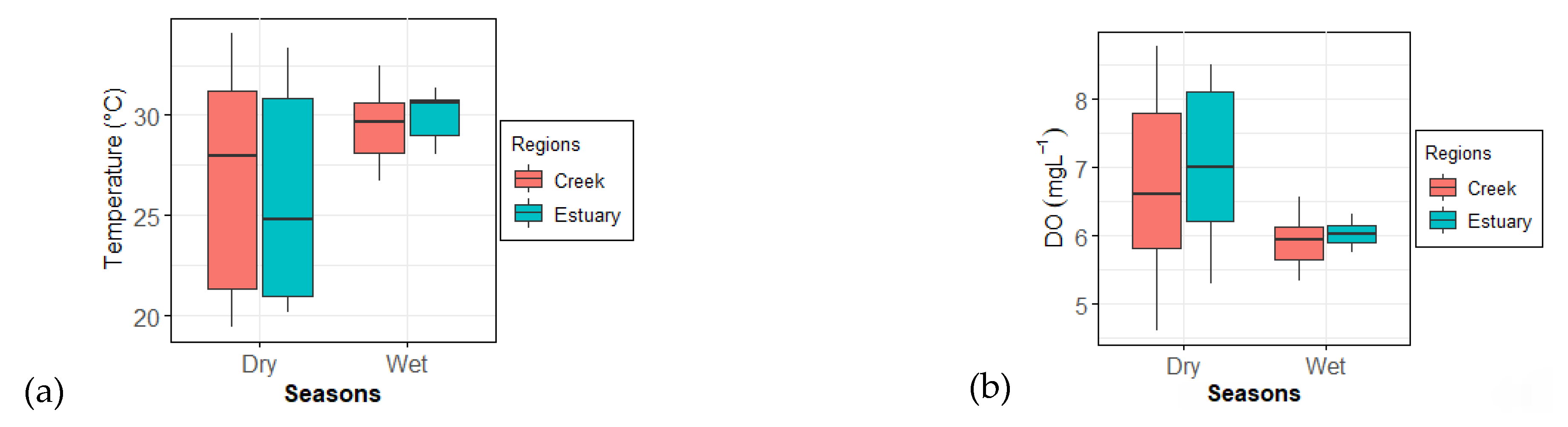
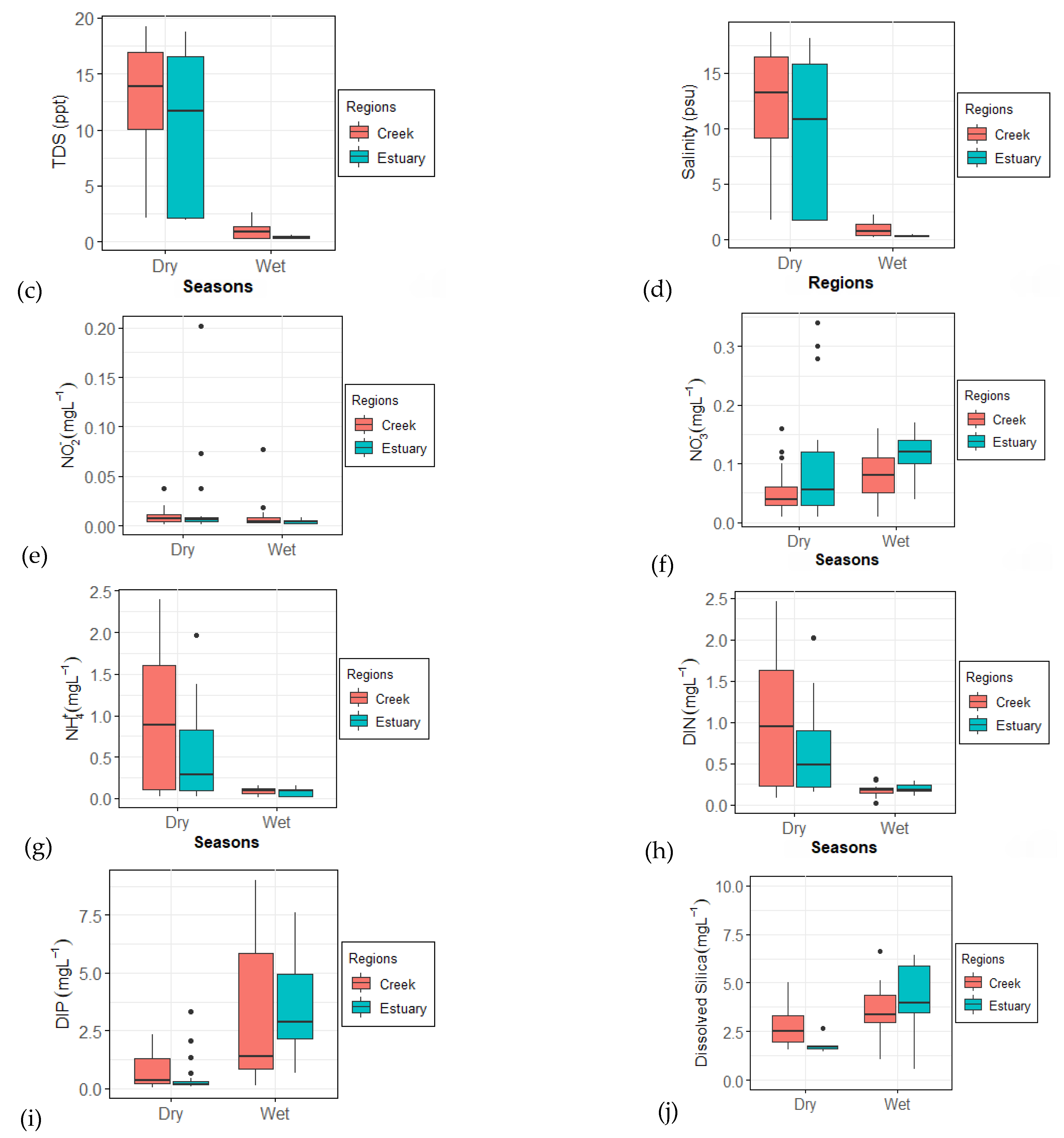
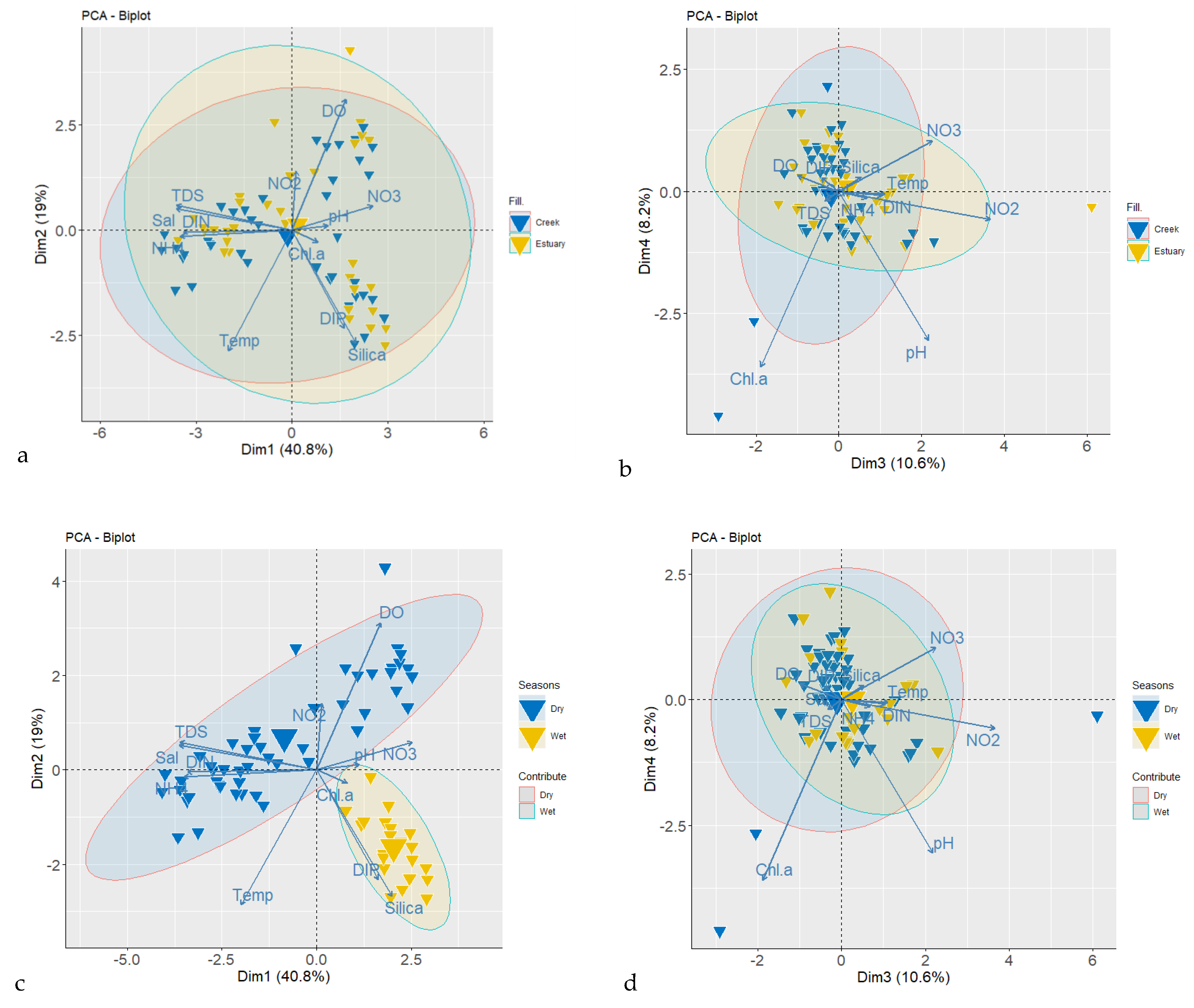
3.1. Physicochemical Parameters

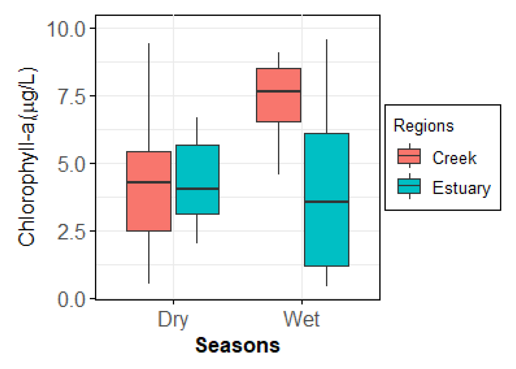
Salinity near the coast and within the estuary varies over a number of different timescales (

Table 1. Two-way analysis of variance for differences of ecologically important parameters on sampling stations and sampling months for the survey in the tidal mangrove creeks of the PRE. F indicates the likelihood ratio; p indicates the probability.

	Creeks				Estuary vs. Creeks
	Stations		Seasons (Dry and Wet)		Stations		Seasons (Dry and Wet)
	F	p	F	p	F	p	F	p
Temperature	0.079	0.995	1.953	0.169	1.303	0.257	6.126	0.015
Salinity	0.585	0.712	367.421	0.000	0.172	0.679	731.852	0.000
DO	0.585	0.712	0.130	0.720	3.720	0.057	2.704	0.103
pH	1.589	0.183	0.812	0.372	3.364	0.070	3.675	0.058
Nitrate	0.664	0.652	22.016	0.000	9.199	0.003	43.629	0.000
Nitrite	0.494	0.779	0.000	0.996	0.594	0.443	2.983	0.087
Ammonia	0.813	0.547	47.047	0.000	3.465	0.066	82.945	0.000
Phosphate	0.395	0.850	8.385	0.006	0.928	0.338	13.610	0.000
TDS	0.660	0.656	422.152	0.000	0.069	0.793	831.264	0.000
DIN	0.814	0.546	43.214	0.000	2.297	0.133	72.760	0.000
Chlorophyll a	0.978	0.442	1.058	0.309	7.799	0.006	0.714	0.400
Silica	7.336	0.014	22.86	0.000	104.89	0.000	341.64	0.000

). The salinity level varies with the season. Salinity ranged from 0.18 to 18.66 psu with an average of 8.34 psu in the study areas. The highest concentrations of salinity were found in the dry season (1.66–18.66 psu) (p < 0.0001) with an average value of 11.43 ± 3.05 psu, whereas the wet season showed the highest salinity (0.18–1.84 psu) with an average value of 0.62 ± 0.11 psu in the tidal mangrove creeks and the PRE (

Table 2. Average, standard error, maximum, and minimum values of different environmental and chlorophyll a parameter distribution in the PRE.

Dry Season (Non-Monsoon) (n = 25)
ST	Temp (°C)	DO (mg/L)	pH	Sal (psu)	TDS (ppt)	Nitrate (mg/L)	Nitrite (mg/L)	Ammonia (mg/L)	DIN (mg/L)	DIP (mg/L)	Chlorophyll a (µg/L)	Silica (mg/L)
E1	26.07 ± 2.59 31.30 − 20.4	6.98 ± 0.61 8.23 − 5.35	7.75 ± 0.08 7.91 − 7.49	11.57 ± 3.22 17.84 − 1.77	12.43 ± 3.33 18.66 − 2.17	0.009 ± 0.002 0.02 − 0.001	0.048 ± 0.02 0.13 − 0.01	0.61 ± 0.25 1.18 − 0.03	0.67 ± 0.25 1.22 − 0.17	0.20 ± 0.025 0.29 − 0.14	3.99 ± 0.77 6.48 − 2.8	2.65 ± 0.05 2.80 − 2.51
E2	25.97 ± 2.47 31.09 − 20.8	6.88 ± 0.61 8.5 − 5.48	7.69 ± 0.7 7.87 − 7.47	11.64 ± 3.25 17.67 − 1.68	12.36 ± 3.30 18.35 − 2.08	0.005 ± 0.001 0.01 − 0.001	0.064 ± 0.02 0.14 − 0.02	0.81 ± 0.25 1.97 − 0.12	0.87 ± 0.35 2.02 − 0.22	0.22 ± 0.06 0.43 − 0.12	4.004 ± 0.69 6.19 − 2.35	1.48 ± 0.03 1.57 − 1.39
E3	26.27 ± 2.60 31.61 − 20.8	6.73 ± 0.58 8.02 − 5.3	7.62 ± 0.12 7.94 − 7.35	11.42 ± 3.15 17.35 − 1.66	12.18 ± 3.25 18.05 − 2.03	0.005 ± 0.001 0.01 − 0.001	0.1 ± 0.03 0.28 − 0.02	0.44 ± 0.15 0.78 − 0.13	0.54 ± 0.12 0.82 − 0.24	0.17 ± 0.02 0.23 − 0.12	4.004 ± 0.72 6.29 − 2.28	1.78 ± 0.041 1.89 − 1.67
E4	26.53 ± 2.5 31.4 − 21	6.78 ± 0.45 8.12 − 5.76	7.69 ± 0.11 7.93 − 7.42	10.94 ± 3.03 16.12 − 1.72	11.89 ± 3.09 17.15 − 2.09	0.01 ± 0.007 0.04 − 0.001	0.07 ± 0.02 0.14 − 0.02	0.74 ± 0.25 1.38 − 0.1	0.82 ± 0.25 1.47 − 0.24	0.45 ± 0.10 1.34 − 0.12	4.64 ± 0.71 6.69 − 3.07	1.59 ± 0.02 1.65 − 1.5
E5	26.49 ± 2.57 31.94 − 20.5	6.73 ± 0.5 8.11 − 5.4	7.66 ± 0.08 7.85 − 7.43	10.83 ± 2.89 15.64 − 1.71	11.95 ± 3.02 16.66 − 2.1	0.006 ± 0.0015 0.01 − 0.001	0.05 ± 0.015 0.12 − 0.02	0.57 ± 0.18 0.98 − 0.03	0.63 ± 0.17 1.01 − 0.16	0.22 ± 0.08 0.5 − 0.1	4.13 ± 0.54 5.79 − 3.1	1.71 ± 0.025 1.79 − 1.63
Wet season (monsoon) (n = 10)
ST	Temp (°C)	DO (mg/L)	pH	Sal (psu)	TDS (ppt)	Nitrate (mg/L)	Nitrite (mg/L)	Ammonia (mg/L)	DIN (mg/L)	DIP (mg/L)	Chlorophyll a (µg/L)	Silica (mg/L)
E1	30.35 ± 0.38 30.9 − 29.8	6.04 ± 0.06 6.13 − 5.96	8 ± 0.045 8.07 − 7.93	0.21 ± 0.015 0.23 − 0.18	0.38 ± 0.09 0.51 − 0.25	0.002 ± 0.00035 0.003 − 0.001	0.16 ± 0.007 0.17 − 0.15	0.06 ± 0.02 0.11 − 0.01	0.22 ± 0.04 0.28 − 0.16	3.4 ± 0.77 4.5 − 2.3	3.65 ± 1.27 6.16 − 1.14	5.43 ± 0.03 5.47 − 5.38
E2	30.35 ± 0.53 31.1 − 29.6	5.95 ± 0.13 6.15 − 5.76	7.74 ± 0.20 8.03 − 7.46	0.27 ± 0.06 0.36 − 0.19	0.36 ± 0.075 0.47 − 0.25	0.006 ± 0.001 0.01 − 0.001	0.14 ± 0.0005 0.14 − 0.12	0.06 ± 0.02 0.11 − 0.01	0.206 ± 0.03 0.25 − 0.16	3.25 ± 0.75 4.33 − 2.17	3.65 ± 1.13 5.96 − 1.34	3.59 ± 0.04 3.65 − 3.53
E3	30.25 ± 0.6 31.1 − 29.4	6.05 ± 0.13 6.25 − 5.86	7.95 ± 0.08 8.08 − 7.83	0.28 ± 0.014 0.3 − 0.26	0.42 ± 0.05 0.5 − 0.34	0.004 ± 0.0005 0.01 − 0.001	0.085 ± 0.03 0.13 − 0.04	0.085 ± 0.03 0.13 − 0.04	0.174 ± 0.0005 0.18 − 0.16	4.65 ± 1.25 6.43 − 2.87	4.99 ± 1.23 9.56 − 0.42	6.38 ± 0.035 6.44 − 6.33
E4	30.5 ± 0.77 31.6 − 29.4	5.97 ± 0.13 6.17 − 5.78	7.84 ± 0.14 8.05 − 7.63	0.28 ± 0.05 0.36 − 0.21	0.38 ± 0.07 0.49 − 0.28	0.005 ± 0.0005 0.01 − 0.001	0.09 ± 0.015 0.12 − 0.07	0.1 ± 0.00005 0.1 − 0.001	0.2 ± 0.007 0.23 − 0.17	4.6 ± 1.58 7.6 − 1.71	8.12 ± 2.15 15.46 − 0.79	1.86 ± 0.96 3.23 − 0.5
E5	30.7 ± 1.13 32.3 − 29.1	6.13 ± 0.13 6.32 − 5.95	7.63 ± 0.26 8.01 − 7.26	0.83 ± 0.26 1.2 − 0.46	0.46 ± 0.10 0.61 − 0.31	0.003 ± 0.001 0.01 − 0.001	0.1 ± 0.0005 0.11 − 0.09	0.05 ± 0.015 0.1 − 0.01	0.15 ± 0.035 0.22 − 0.1	1.39 ± 0.52 2.13 − 0.66	5.19 ± 0.73 6.24 − 4.16	5.11 ± 0.81 6.27 − 3.96

ST: Station; Temp: Temperature; DO: Dissolved Oxygen; Sal: Salinity; TDS: Total dissolved solids; DIN: Dissolved Inorganic Nitrogen; DIP: Dissolved Inorganic Phosphate.

and

Table 3. Average, standard error, maximum, and minimum values of different environmental and chlorophyll a parameter distribution in the tidal mangrove creeks.

Dry Season (Non-Monsoon) (n = 30)
ST	Temp (°C)	DO (mg/L)	pH	Sal (psu)	TDS (ppt)	Nitrate (mg/L)	Nitrite (mg/L)	Ammonia (mg/L)	DIN (mg/L)	DIP (mg/L)	Chlorophyll a (µg/L)	Silica (mg/L)
C1, C2	26.13 ± 2.75 31.9 − 20.2	6.78 ± 0.6 8.03 − 5.32	7.74 ± 0.09 7.98 − 7.53	11.56 ± 3.23 17.84 − 1.75	12.23 ± 3.23 18.45 − 2.14	0.009 ± 0.0015 0.01 − 0.001	0.05 ± 0.009 0.08 − 0.04	0.96 ± 0.27 2.11 − 0.07	1.03 ± 0.45 2.15 − 0.14	0.99 ± 0.37 2.1 − 0.06	3.51 ± 0.59 4.84 − 2.13	5.01 ± 0.05 5.16 − 4.86
C3, C4	26.04 ± 2.9 32.3 − 19.4	6.42 ± 0.69 8.23 − 4.62	7.63 ± 0.08 7.8 − 7.4	12.52 ± 3.06 18.66 − 3.59	11.45 ± 2.75 19.2 − 4.22	0.014 ± 0.004 0.02 − 0.001	0.05 ± 0.021 0.12 − 0.02	1.16 ± 0.45 2.17 − 0.02	1.23 ± 0.44 2.22 − 0.12	0.66 ± 0.23 1.31 − 0.11	5.08 ± 1.91 11.05 − 0.78	1.55 ± 0.05 1.71 − 1.41
C5, C6	26.06 ± 2.71 31.2 − 20.1	6.35 ± 0.56 8.08 − 5.01	7.61 ± 0.07 7.81 − 7.5	11.73 ± 3.05 17.55 − 2.63	12.47 ± 3.07 18.23 − 3.15	0.006 ± 0.0015 0.01 − 0.001	0.044 ± 0.01 0.12 − 0.01	1.05 ± 0.28 1.61 − 0.08	1.11 ± 0.27 1.63 − 0.21	0.64 ± 0.23 1.26 − 0.16	4.98 ± 1.07 7.44 − 2.49	1.99 ± 0.05 2.14 − 1.85
C7, C8	26.51 ± 2.62 31.7 − 20.65	6.70 ± 0.05 8.18 − 5.51	7.64 ± 0.07 7.77 − 7.48	11.12 ± 2.64 15.49 − 3.0	11.68 ± 2.88 16.16 − 2.43	0.004 ± 0.001 0.01 − 0.001	0.05 ± 0.01 0.1 − 0.03	0.51 ± 0.13 0.75 − 0.05	0.56 ± 0.12 0.80 − 0.15	0.55 ± 0.20 1.29 − 0.13	4.73 ± 1.37 9.41 − 2.17	3.41 ± 0.05 3.56 − 3.26
C9, C10	26.66 ± 2.72 32.5 − 21	7.18 ± 0.69 8.77 − 5.76	7.62 ± 0.12 7.85 − 7.3	11.12 ± 3.05 16.48 − 1.71	11.85 ± 3.10 17.14 − 2.12	0.006 ± 0.001 0.01 − 0.001	0.06 ± 0.015 0.11 − 0.03	0.86 ± 0.25 2.32 − 0.09	0.93 ± 0.35 2.36 − 0.21	0.69 ± 0.22 1.97 − 0.17	9.84 ± 1.71 33.26 − 0.5	1.94 ± 0.05 2.1 − 1.82
C11, C12	26.77 ± 2.81 32.95 − 20.7	6.95 ± 0.5 8.26 − 5.78	7.70 ± 0.09 7.88 − 7.47	11.35 ± 3.08 16.59 − 1.75	11.95 ± 3.1 17.32 − 2.14	0.010 ± 0.004 0.03 − 0.001	0.07 ± 0.025 0.16 − 0.03	0.73 ± 0.30 1.33 − 0.08	0.81 ± 0.25 1.41 − 0.12	0.47 ± 0.18 1.3 − 0.17	6.69 ± 2.52 15.61 − 3.55	3.07 ± 0.05 3.22 − 2.92
Wet season (monsoon) (n = 12)
ST	Temp (°C)	DO (mg/L)	pH	Sal (psu)	TDS (ppt)	Nitrate (mg/L)	Nitrite (mg/L)	Ammonia (mg/L)	DIN (mg/L)	DIP (mg/L)	Chlorophyll a (µg/L)	Silica (mg/L)
C1, C2	29.95 ± 0.7 30.9 − 28.95	6.12 ± 0.16 6.35 − 5.88	7.83 ± 0.54 7.96 − 7.7	0.22 ± 0.02 0.26 − 0.18	0.28 ± 0.02 0.32 − 0.25	0.023 ± 0.01 0.04 − 0.001	0.12 ± 0.01 0.14 − 0.1	0.06 ± 0.015 0.1 − 0.02	0.19 ± 0.025 0.24 − 0.15	2.74 ± 0.72 4.47 − 1.01	7.35 ± 0.005 7.36 − 7.35	2.73 ± 1.18 4.4 − 1.06
C3, C4	30.25 ± 0.45 30.9 − 29.6	5.97 ± 0.09 6.11 − 5.85	7.67 ± 0.15 7.89 − 7.46	0.55 ± 0.24 0.9 − 0.22	0.61 ± 0.24 0.96 − 0.27	0.004 ± 0.0003 0.006 − 0.002	0.057 ± 0.015 0.08 − 0.04	0.06 ± 0.015 0.09 − 0.04	0.12 ± 0.03 0.17 − 0.07	4.76 ± 1.08 8.44 − 1.1	9.73 ± 0.59 10.57 − 8.9	4.12 ± 0.70 5.11 − 3.12
C5, C6	29.77 ± 0.8 30.9 − 28.65	5.73 ± 0.08 5.85 − 5.61	7.52 ± 0.25 7.87 − 7.17	0.97 ± 0.08 1.1 − 0.85	1.03 ± 0.26 1.41 − 0.66	0.007 ± 0.0001 0.01 − 0.01	0.08 ± 0.02 0.11 − 0.05	0.11 ± 0.01 0.13 − 0.09	0.19 ± 0.03 0.25 − 0.15	1.27 ± 0.22 1.6 − 0.95	7.57 ± 0.09 7.71 − 7.43	3.59 ± 0.04 3.66 − 3.53
C7, C8	29.92 ± 1.6 32.2 − 27.65	5.69 ± 0.19 5.98 − 5.42	7.73 ± 0.04 7.8 − 7.67	1.36 ± 0.33 1.84 − 0.88	2.87 ± 0.40 3.45 − 2.3	0.009 ± 0.003 0.02 − 0.001	0.05 ± 0.02 0.1 − 0.02	0.08 ± 0.0005 0.09 − 0.06	0.15 ± 0.02 0.18 − 0.12	3.09 ± 1.39 6.04 − 0.16	9.04 ± 0.85 10.25 − 7.84	3.33 ± 0.64 4.25 − 2.42
C9, C10	30.15 ± 0.95 31.5 − 28.8	6.13 ± 0.14 6.34 − 5.93	7.64 ± 0.12 7.82 − 7.47	0.54 ± 0.06 0.64 − 0.45	0.66 ± 0.06 0.76 − 0.56	0.006 ± 0.0015 0.01 − 0.001	0.09 ± 0.01 0.11 − 0.08	0.15 ± 0.0005 0.2 − 0.1	0.19 ± 0.005 0.21 − 0.18	2.57 ± 1.15 4.91 − 0.24	9.07 ± 0.8 10.2 − 7.95	4.78 ± 1.3 6.63 − 2.94
C11, C12	29.17 ± 1.04 30.65 − 27.7	5.82 ± 0.22 6.13 − 5.52	7.75 ± 0.01 7.77 − 7.73	1.28 ± 0.15 1.5 − 1.06	0.41 ± 0.05 0.49 − 0.34	0.006 ± 0.002 0.01 − 0.001	0.08 ± 0.03 0.14 − 0.04	0.09 ± 0.02 0.14 − 0.06	0.19 ± 0.01 0.21 − 0.17	3.50 ± 1.55 6.27 − 0.75	11.41 ± 1.23 13.17 − 9.66	3.04 ± 0.02 3.07 − 3.01

ST: Station; Temp: Temperature; DO: Dissolved Oxygen; Sal: Salinity; TDS: Total dissolved solids; DIN: Dissolved Inorganic Nitrogen; DIP: Dissolved Inorganic Phosphate.

). Salinity was higher in the tidal mangrove creeks at 12.26 psu (0.87 psu) than the PRE at 9.46 psu (0.29 psu) during the dry (wet) season, respectively (Figure 2d). The concentration of salinity was higher in the PRE compared to tidal mangrove creeks. During the wet season, water temperatures in the Morapasur channel ranged from 26.7 °C to 32.4 °C, with an average of 29.1 ± 0.81 °C. The dry season exhibited a relatively higher range from 19.4 °C to 34.1 °C in the Koromjal channel, with an average value of 26.7 ± 2.65 °C. Water temperature was low during the dry winter months following the post-monsoon season and high during the wet period. During the dry season, water temperature in the tidal mangrove creeks (27.3 °C) was significantly (p < 0.015) higher (Table 1) than in the PRE (25.6 °C) (Table 2 and Table 3). During the wet season, the PRE (30.03 °C) had higher water temperatures than the tidal mangrove creeks (29.4 °C) (Figure 2a).

Dissolved oxygen (DO) at the study locations ranged from 4.62 to 8.77 mg/L with an average of 6.54 mg/L. DO concentrations were found to be higher during the dry season (6.77 ± 0.53 mg/L) (p < 0.057) (Table 1), than during the wet season (5.96 ± 0.13 mg/L) in the tidal mangrove creeks and the PRE due to higher temperatures being observed during the wet season and lower temperatures being observed during the dry season (Table 2 and Table 3). The DO concentration was higher in the PRE at 7.1 mg/L during the dry season and 6.03 mg/L during the wet season than in the tidal mangrove creeks at 6.65 mg/L during the dry season and 5.92 mg/L during the wet season (Figure 2b). The pH value was higher during the wet season (7.75 ± 0.16) compared to the dry season (7.66 ± 0.14) (Table 2 and Table 3). During the dry season, pH values were, respectively, 7.5 and 7.6 in the PRE and mangrove creeks. On the other hand, during the wet season, pH values were 7.8 and 7.7 in the PRE and mangrove creeks, respectively.

Dissolved inorganic nitrogen (DIN) at the study locations ranged from 0.07 to 2.32 mg/L, with an average value of 0.65 mg/L. Average DIN concentrations were significantly (p < 0.0001) higher in the tidal mangrove creeks (0.71 mg/L) than in the PRE (0.57 mg/L) (Table 1). Higher concentrations of dissolved inorganic nitrogen were found during the dry season (0.84 ± 0.27 mg/L), whereas the wet season showed lower dissolved inorganic nitrogen (0.18 ± 0.02 mg/L) in the tidal mangrove creeks and the PRE (Table 2 and Table 3). During the dry season, dissolved inorganic nitrogen was higher in the tidal mangrove creeks (1.02 mg/L) than in the PRE (0.62 mg/L). During the wet season, dissolved inorganic nitrogen was higher in the PRE (0.20 mg/L) than in the tidal mangrove creeks (0.18 mg/L) (Figure 2h).

Dissolved inorganic phosphate (DIP) at the study locations ranged from 0.06 to 8.44 mg/L with an average of 1.30 mg/L. The average DIP concentration was significantly (p < 0.0001) higher (Table 1) in the tidal mangrove creeks (1.35 mg/L) than in PRE (1.25 mg/L). Higher concentrations of dissolved inorganic phosphate were found during the wet season (3.20 ± 0.99 mg/L), whereas during the dry season showed lower dissolved inorganic phosphate (0.48 ± 0.15 mg/L) in the tidal mangrove creeks and the PRE (Table 2 and Table 3). During the dry season, dissolved inorganic phosphate was higher in the tidal mangrove creeks (0.72 mg/L) than in the PRE (0.48 mg/L) whereas during the wet season, dissolved inorganic phosphate was higher in the PRE (3.65 mg/L) than in the tidal mangrove creeks (2.94 mg/L) (Figure 2i). Among the different nutrient species, DIN (F = 43.214, p < 0.05) and DIP (F = 8.385, p < 0.0001) varied more temporarily than spatially.

The average dissolved silica concentration was higher in the tidal mangrove creeks (3.24 mg/L) than in the PRE (2.84 mg/L). During the dry season, dissolved silica concentrations were significantly higher (p < 0.0001) (Table 1) in the tidal mangrove creeks (2.84 ± 0.05 mg/L) than in the PRE (1.64 ± 0.03 mg/L) (Table 2 and Table 3). In contrast, during the wet season, dissolved silica concentrations were higher in the PRE (4.02 ± 0.44 mg/L) than in the tidal mangrove creeks (3.66 ± 0.65 mg/L) (Figure 2j). Dissolved silica showed significant differences (p < 0.0001) between PRE and the tidal mangrove creeks spatially and temporarily (Table 1).

3.2. Chlorophyll a

Chlorophyll a ranged from 0.42 to 33.26 µg/L, with an average of 5.68 µg/L. Higher values of chlorophyll a were obtained from mangrove creeks and lower values from the PRE. This trend was visible in both sampling seasons. The average chlorophyll a concentration was higher in tidal mangrove creeks (6.20 µg/L) than in PRE (4.80 µg/L). The average chlorophyll a concentration during the dry season and wet season was, respectively, 4.66 ± 1.14 µg/L and 7.32 ± 0.91 µg/L. Chlorophyll a concentration showed significant spatial differences between the PRE and the mangrove creeks (p < 0.006) but, temporally showed no significant differences (p > 0.400) (Table 1) and higher concentrations of chlorophyll a were found during the wet season (0.42–15.46 µg/L), whereas the dry season showed lower chlorophyll a (0.50–33.26 µg/L) in the tidal mangrove creeks and the PRE (Figure 3).

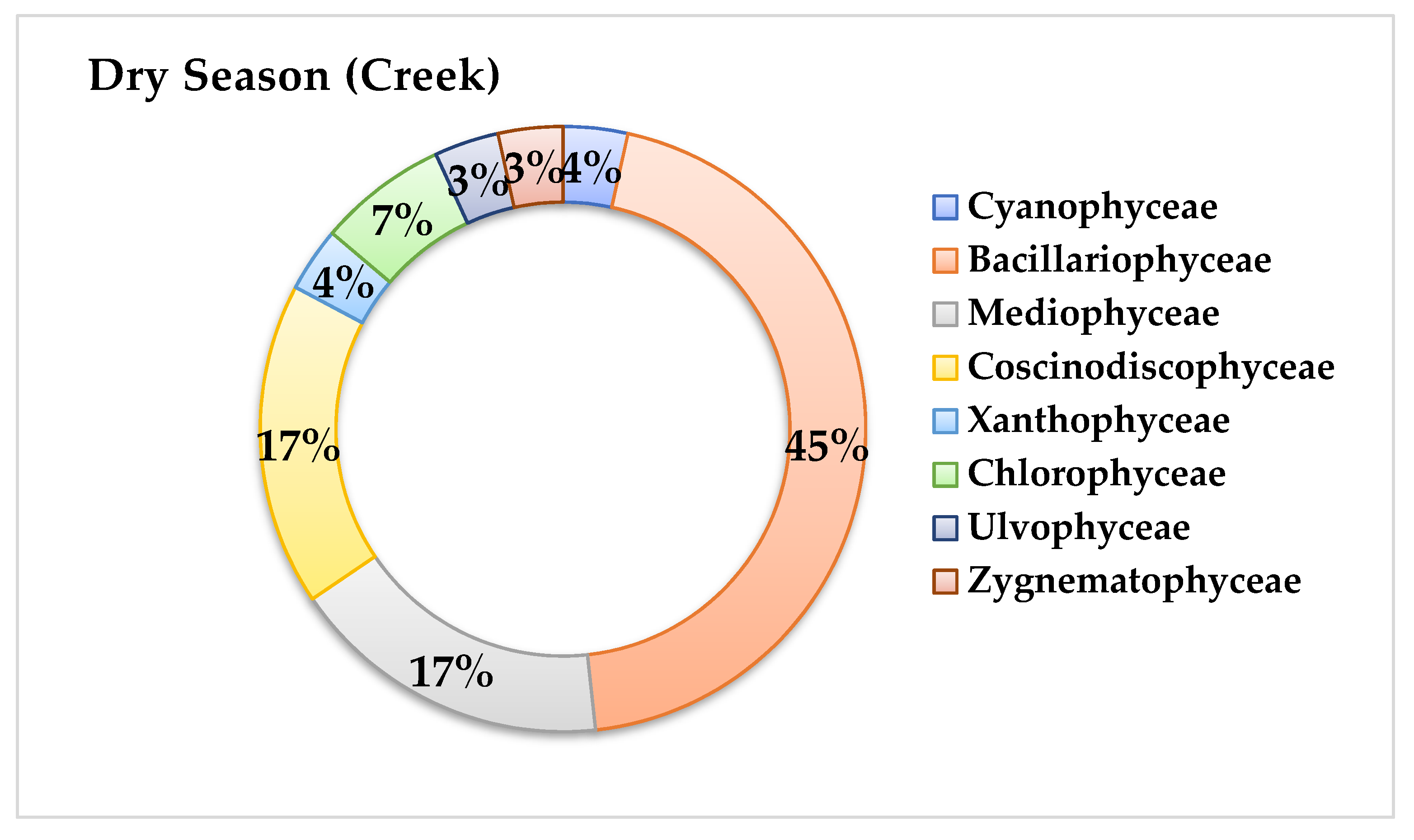
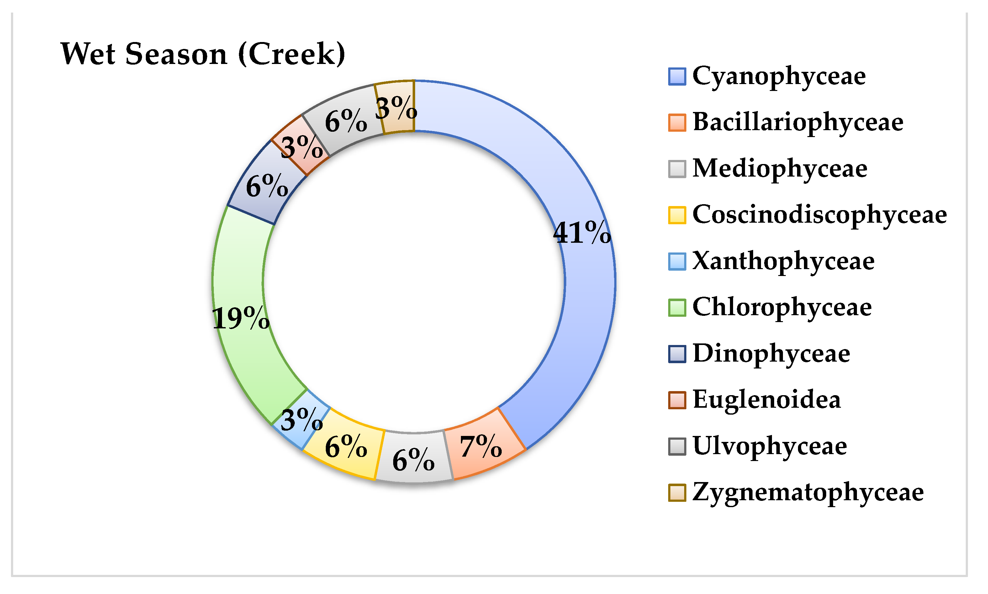
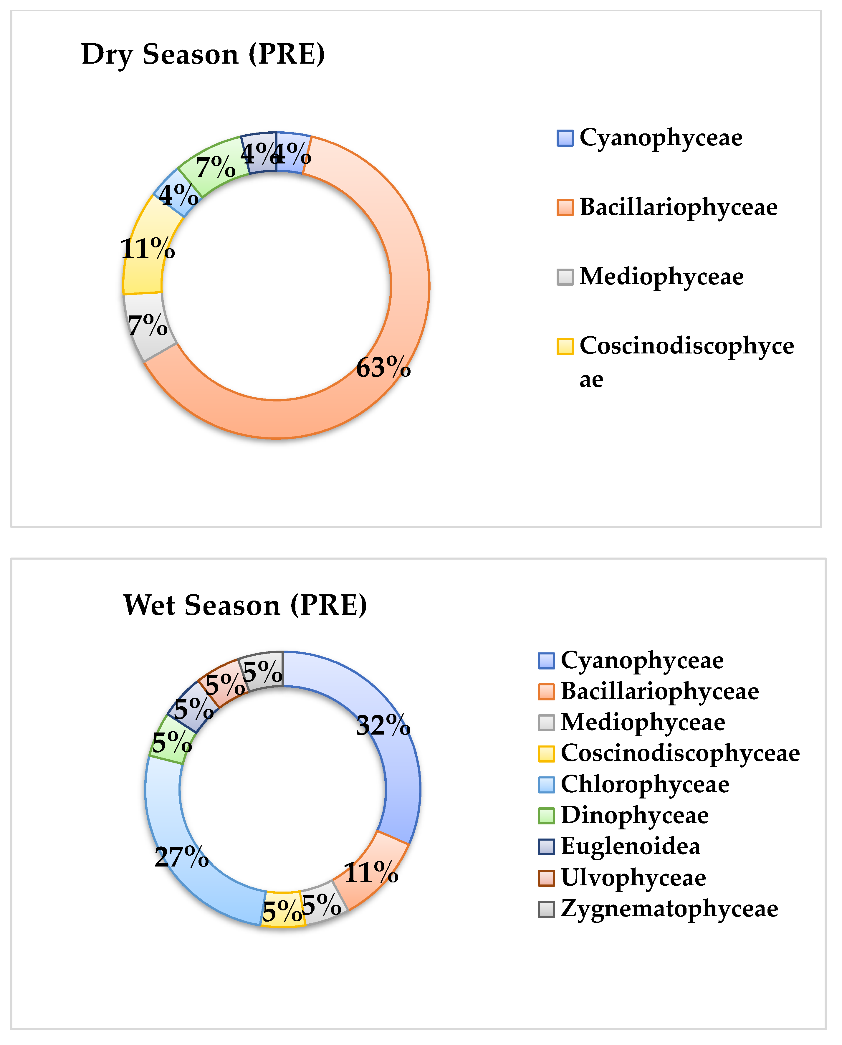
3.3. Phytoplankton Community Structure

In this study, we encountered 38 phytoplankton species, with 11 species in Bacillariophyceae (diatoms), 8 species in Cyanophyceae (blue-green algae), 5 species in Chlorophyceae (green algae), 3 species of Coscinodiscophyceae, 3 species in Mediophyceae, 2 species of Zygnematophyceae, 2 species in Dinophyceae (Dinoflagellates), 2 species in Ulvophyceae, 1 species in Xanthophyceae and 1 species in Euglenophyceae (

Table 4. Presence (+) or absence (blank) of phytoplankton species in the tidal mangrove creeks and the PRE.

Taxon		Sampling Stations
		C1, C2	E1	C3, C4	E2	C5, C6	E3	C11, C12	E4	C9, C10	C7, C8	E5
Cyanophyceae	Oscillatoria sp.	+		+	+					+	+
	Aphanizomenon sp.	+		+		+				+	+
	Gloeocapsa sp.		+				+					+
	Dolichospermum sp.											+
	Merismopedium sp.	+	+	+	+			+	+	+	+	+
	Microcystis sp.	+		+
	Arthrospira sp.			+
	Gomphosphaeria sp.					+	+				+
Bacillariophyceae	Lioloma sp.	+	+	+	+	+		+	+	+	+
	Pleorosigma sp.						+					+
	Asterionella sp.			+							+
	Fragilaria sp.								+
	Diatoma sp.										+
	Chaetoceros sp.											+
	Surirella sp.	+							+
	Thalassionema sp.		+		+
	Nitzschia sp.		+						+
	Navicula sp.											+
	Synedra sp.			+				+				+
Coscinonodiscophyceae	Coscinodiscus sp.	+	+	+	+	+	+	+		+	+	+
	Triceratium sp.				+							+
	Melosira sp.										+
Mediophyceae	Ditylum sp.						+		+	+	+	+
	Odontella sp.										+
	Tropidoneis sp.										+
Xanthophyceae	Tribonema sp.	+		+		+				+	+	+
Chlorophyceae	Stigeoclonium sp.									+
	Hydrodictyon sp.	+	+								+
	Pediastrum sp.							+			+
	Volvox sp.	+
	Oedogonium sp.	+			+	+	+	+
Zygnematophyceae	Spirogyra sp.	+		+	+			+				+
	Mougeotia sp.	+		+
Dinophyceae	Tripos sp.										+
	Polykrikos sp.											+
Ulvophyceae	Cladophora sp.							+
	Ulothrix sp.									+
Euglenophyceae	Euglena sp.		+							+	+

).

In both the dry and wet seasons, Lioloma sp., Coscinodiscus sp., Tribonema sp., Asterionella sp., Thalassionema sp., Oedogonium sp., and Cladophora sp. phytoplankton species were found in both the tidal mangrove creeks and the PRE. Coscinodiscus sp. was found in most of the sampling stations except the estuarine E4 station. Lioloma sp. was found in most of the sampling stations except the estuarine E3 and E5 sampling stations (Table 4).

Phytoplankton abundance in the study area during the dry and wet seasons ranged from 50.8 × 10³ to 66.1 × 10³ and 39.4 × 10³ to 75.9 × 10³ cells /L, respectively. The average phytoplankton abundance was 58.0 × 10³ cells /L. During the dry season, phytoplankton density varied from 42.9 × 10³ to 86.9 × 10³ cells/L with an average of 66.1 × 10³ cells/L in the tidal mangrove creeks and 25.3 × 10³ to 83.6 ×10³ cells/L with an average 50.8 × 10³ cells/L in the PRE. During the wet season, phytoplankton abundance ranged from 27.5 × 10³ to 106.7 × 10³ cells/L with an average of 75.9 × 10³ cells/L in the tidal mangrove creeks and 17.6 × 10³ to 59.4 × 10³ cells/L with an average 39.4 × 10³ cells/L in the PRE. The highest abundance was registered in the tidal mangrove creeks.

In general, diatoms (Bacillariophyceae and Coscinodiscophyceae) were the dominant class, ranging from 25% during the wet season to 68% during the dry season (Figure 4 and Figure 5). On the other hand, blue-green algae (Cyanophyceae) were the dominant class, ranging from 4% during the dry season to 36% during the wet season. Green algae (Chlorophyceae) represented 7% during the dry season and 23% during the wet season. The dominance of diatoms during the dry season was replaced by blue-green algae (Cyanophyceae) during the wet season. The dominance of diatoms did not occur at every sampling station. However, during the dry season, diatoms show significant differences from other phytoplankton groups in the study area. Thus, the seasonal succession of phytoplankton was highly pronounced in the tidal mangrove creeks and the PRE. Overall, diatoms, blue-green algae, and green algae were co-dominant in the study period.

3.4. Phytoplankton Species Diversity

There was no significant variation between the PRE and tidal mangrove creeks (p > 0.05) on the phytoplankton alpha diversity indices during the study period. The results of the t-test showed that the hydrological period showed a significant difference (p < 0.05) but no significant (p > 0.05) differences were observed spatially (

Table 5. The temporal and spatial variation of phytoplankton alpha diversity indices.

		Shannon–Weaver Index	Peilou Index	Margalef Index	Simpson Diversity Index	Simpson’s Reciprocal Index
PRE	Dry season	2.82	0.8	6.32	0.1	9.81
	Wet season	2.68	0.66	6.08	0.19	7.02
Creeks	Dry season	2.91	0.86	6.66	0.07	11.08
	Wet season	3.09	0.97	6.86	0.03	14.57
t-test
Dry × Wet season		p < 0.05	p < 0.05	p < 0.05	p < 0.05	p < 0.05
PRE × Creeks		p > 0.05	p > 0.05	p > 0.05	p > 0.05	p > 0.05

). In the wet season, the Shannon–Weaver diversity index found in the PRE and the connected tidal mangrove creeks was, respectively, 2.68 and 3.09. In the dry season, the Shannon–Weaver diversity index found in the PRE and the tidal mangrove creeks were 2.82 and 2.91, respectively (Table 5). In the tidal mangrove creeks, the Shannon–Weaver diversity index was found to be higher during the wet season compared to the dry season. In contrast, Shannon–Weaver diversity index values were found to be higher during the dry season compared to the wet season in the PRE.

The spatial and temporal distribution of the phytoplankton Pielou index (evenness) was very similar to that of the Shannon–Weaver diversity index. In the wet season, evenness values found in the PRE and the tidal mangrove creeks were 0.66 and 0.97 (Table 5). In the dry season, evenness values found in the PRE and the tidal mangrove creeks were 0.80 and 0.86, respectively. Similarly, in the Shannon–Weaver diversity index and Pielou index, there was significant (p < 0.05) variation in the Margalef index (species diversity) in different hydrological periods. In the wet season, species richness was found in the PRE and the tidal mangrove creeks at 6.08 and 6.86, respectively (Table 5). In the dry season, species richness was found in the PRE and the tidal mangrove creeks at 6.32 and 6.66, respectively (Table 5). The Simpson’s diversity indices and Simpson’s reciprocal indices (1/D) in the tidal mangrove creeks and PRE were 0.05, 12.82 and 0.14, 8.4, respectively (Table 5).

The multivariate analysis (PCA) test showed a seasonal gradient for the water quality parameters and phytoplankton, forming two different groups for the dry and wet seasons (Figure 6c,d and Figure 7c,d). PCA showed that four principal components explained 78.6% of the total variance for the environmental variables (Figure 6a–d). The main parameters in PC1 were salinity, total dissolved solids, NH₄⁺, and DIN, which contributed 40.8% of the total variance and silica, DO, water temperature, and DIP were the main parameters in PC2, contributing to 19% of the total variance (Figure 6a,b). The rest of the cumulative variation in PC3 and PC4 (Figure 6c,d) was contributed by NO₂^_, NO₃^_, pH, DO, silica, DIP, and water temperature.

Similarly, PCA showed that four principal components explained 71.2% of the total variance for the phytoplankton community (Figure 7a–d). In PC1, Bacillariphyceae, Coscinodiscophyceae, Mediophyceae, and Xanthophyceae were the main parameters, contributing to 28.6% of the total variance and Cyanophyceae, Chlorophyceae, and Ulvophyceae were the main parameters in PC2, contributing to 21.1% of the total variance (Figure 7a,b). Chlorophyceae, Zygnematophyceae, Dinophyceae, and Ulvophyceae contributed to the rest of the cumulative variation in PC3 and PC4 (Figure 7c,d). The hierarchical clustering amongst the environmental parameters and phytoplankton abundance showed four groups; each was clearly associated with a specific season (Figure 8). As shown by the dendrogram (Figure 8), distinct clusters of dry vs. wet and creek vs. estuarine environmental parameters showed distinct patterns.

The distinct distribution of environmental variables and phytoplankton in different study sites is shown by non-metric multidimensional scaling (NMDS) (Figure 9). ANOSIM of the overall combination of environmental variables and phytoplankton in all study sites across all seasons revealed that there were significant differences observed in the dry and wet seasons (p < 0.05) with a high range value of R = 0.59 but no significant difference observed between the sampling sites (p > 0.05) with R = 0.002.

The SIMPER routine was analyzed based on the abundance of phytoplankton described by the discriminating species. The seasonal average dissimilarity was 85.13 and the spatial average dissimilarity was 74.93.

Table 6. SIMPER analysis depicted the ‘discriminating species’ that contribute to the maximum dissimilarity between the assemblages (sampling sites) and (seasons).

Avg. Dissimilarity	Discriminating Species (Average Dissimilarity and Contribution Percentage)
Dry vs. Wet (85.13)	Synedra sp. (3.90, 4.58%), Fragilaria sp. (3.73, 4.39%), Asterionella sp. (3.66, 4.30%), Pleorosigma sp. (3.57, 4.19%), Coscinodiscus sp. (3.55, 4.17%), Diatoma sp. (3.54, 4.16%), Lioloma sp. (3.25, 3.81%), Arthrospira sp. (3.18, 3.74%), Merismopedium sp. (3.17, 3.73%), Chaetoceros sp. (3.04, 3.58%), Ulothrix sp. (2.93, 3.44%), Microcystis sp. (2.85, 3.34%), Pediastrum sp. (2.82, 3.31%), Oedogonium sp. (2.80, 3.29%), Melosira sp. (2.67, 3.14%), Gomphosphaeria sp. (2.67, 3.14%), Triceratium sp. (2.63, 3.1%), Nitzschia sp. (2.50, 2.94%), Aphanizomenon sp. (2.28, 2.68%), Gloeocapsa sp. (2.22, 2.61%), Stigeoclonium sp. (2.22, 2.60%), Ditylum sp. (2.18, 2.56%), Oscillatoria sp. (2.17, 2.55%), Muogeotia sp. (2.05, 2.41%), Odontella sp. (1.81, 2.12%), Dolichospermum sp. (1.80, 2.12%), Spirogyra sp. (1.67, 1.97%), Hydrodictyon sp. (1.66, 1.95%), Volvox sp. (1.43, 1.68%), Tropidoneis sp. (1.28, 1.51%), Surirella sp. (1.27, 1.49%), Navicula sp. (1.26, 1.48%), Thalassionema sp. (1.23, 1.44%), Tribonema sp. (1.04, 1.22%), Cladophora sp. (0.37, 0.43%), Euglena sp. (0.29, 0.35%), Tripos sp. (0.14, 0.16%) and Polykrikos sp. (0.13, 0.16%).
Creek vs. Estuary (74.93)	Synedra sp. (3.89, 5.19%), Diatoma sp. (3.63, 4.85%), Asterionella sp. (3.48, 4.65%), Coscinodiscus sp. (3.46, 4.61%), Fragilaria sp. (3.39, 4.53%), Lioloma sp. (3.38, 4.52%), Pleorosigma sp. (3.20, 4.27%), Chaetoceros sp. (3.06, 4.09%), Nitzschia sp. (2.91, 3.89%), Triceratium sp. (2.78, 3.71%), Melosira sp. (2.75, 3.67%), Pediastrum sp. (2.48, 3.31%), Gomphosphaeria sp. (2.31, 3.09%), Ulothrix sp. (2.27, 3.03%), Arthrospira sp. (2.25, 3.01%), Ditylum sp. (2.18, 2.92%), Odontella sp. (2.14, 2.86%), Oedogonium sp. (2.02, 2.70%), Muogeotia sp. (1.99, 2.65%), Microcystis sp. (1.70, 2.27%), Merismopedium sp. (1.63, 2.18%), Stigeoclonium sp. (1.50, 2.0%), Hydrodictyon sp. (1.50, 2.0%), Surirella sp. (1.49, 1.98%), Navicula sp. (1.48, 1.97%), Tropidoneis sp. (1.43, 1.92%), Thalassionema sp. (1.39, 1.86%), Spirogyra sp. (1.25, 1.68%), Aphanizomenon sp. (1.24, 1.66%), Gloeocapsa sp. (1.23, 1.64%), Volvox sp. (1.22, 1.63%), Oscillatoria sp. (1.21, 1.61%), Tribonema sp. (1.11, 1.49%), Dolichospermum sp. (1.01, 1.35%), Cladophora sp. (0.36, 0.48%), Tripos sp. (0.18, 0.24%), Euglena sp. (0.17, 0.23%) and Polykrikos sp. (0.08, 0.12%).

summarizes the information on characterized species and their percentage contribution to the total phytoplankton abundance in each group. Synedra sp. (4.58%), Fragilaria sp. (4.39%), Asterionella sp. (4.30%), Pleorosigma sp. (4.19%), Coscinodiscus sp. (4.17%) and Diatoma sp. (4.16) were the major contributors to the seasonal changes. Similarly, Synedra sp. (5.19%), Diatoma sp. (4.85%), Asterionella sp. (4.65%), Coscinodiscus sp. (4.61%), Fragilaria sp. (4.53%), Lioloma sp. (4.52%), Pleorosigma sp. (4.27%) and Chaetoceros sp. (4.09%) were the major contributors to the spatial changes. With that percentage contribution in the different assemblages, these species were exhibited as key phytoplankton species that differentiated between the assemblages, and their variability makes them discriminating species in the different phytoplankton assemblages.

4. Discussion

4.1. Physicochemical Parameters

Salinity is the key indicator of an estuary’s health and salt content increased steadily to a maximum during the winter dry season and then decreased significantly during the rainy season. Changes in salinity significantly affected the diatom growth. In addition, salinity has been reported as a major factor associated with shifts in phytoplankton community structure in mangrove ecosystems [5]. In fact, diatoms are more prevalent in estuarine areas due to high salinity and give way to green algae in upstream areas when the salinity becomes low. In this study, the higher salinity value was observed in the dry season due to higher atmospheric temperature, low rainfall, decreased freshwater discharge, and higher evaporation [38]. In contrast, low salinity during the wet season is due to the influx of freshwater runoff [39,40]. At high tide, the water from the Bay of Bengal penetrates the estuary zone and contributes to increasing the salinity; at low tide, the influence of freshwater runoff from upstream rivers reduces the salinity of the study area during low tide conditions of the study area. Salinity concentration was higher in the mangrove creeks than in the main PRE all year round. This may be due to the presence of tidal salt flats within the tidal mangrove creeks.

Water temperature plays a crucial role in the distribution of living organisms and the rate of photosynthesis in the aquatic environment [41,42]. The rates of photosynthesis appear to be dropping by 37 °C [38]. Temperature is the most important factor in maintaining the growth, reproduction, survival, and distribution of organisms in the physical environment. Because the temperature of the estuarine water is controlled by the temperature of the atmosphere [43]. Temperature controls the behavioral characteristics of organisms and the solubility of gases and salts in water [43]. In tropical estuarine ecosystems, rainfall plays an important role in the seasonal variability of water temperature, salinity, DO, TDS, and chlorophyll a concentration. The temperature of the water is usually influenced by the intensity of solar radiation, tidal currents, the inflow of fresh water and atmospheric fluctuations [44,45]. However, high phytoplankton density in the dry season was generally controlled by phosphate and nitrogen. Increased phytoplankton productivity during the dry season was probably due to the favorable environmental conditions related to light, temperature, and nutrient availability [5]. The composition of diatom assemblages was significantly related to shifts in temperature due to warming trends of climate change.

Dissolved oxygen (DO) is a crucial indicator of water quality [46]. High concentrations of dissolved oxygen (DO) were found in the dry season, whereas the wet season showed low DO in the PRE and the tidal mangrove creeks. The higher the water temperature, the lower the solubility of oxygen [47]. High photosynthetic activity and periodic flushing characteristics increase the DO level. The drop in DO levels during the wet season is related to the amount of oxygen-depleting compounds that enter the estuary through runoff from nearby industrial or agricultural areas [48].

The significant spatio-temporal variation of surface water pH can be attributed to factors such as seawater intrusion into the Bangladesh Sundarbans estuaries from the Bay of Bengal; the freshwater contribution from the Bangladesh Sundarbans through several channels, creeks and tributaries of the Gorai Madhumati Rupsha Pasur River System. pH is also an important variable in water quality assessment as it influences many biological and chemical processes [5]. A pH higher than 7 indicates increasing basicity, while values lower than 7 tend towards acidity. Waters with low pH cause the growth and reproduction of aquatic organisms to be limited [5]. However, it can also be a very acidic environment with a pH below 6. A pH that is lower than 7 but higher than 8.5 is not ideal for biological productivity, while a pH lower than 4 is detrimental to aquatic life [45]. In the present study, water pH was within the optimum level.

External inputs of DIN such as nitrates, nitrites, and ammonia are primarily derived from nearby catchment sources and delivered to the estuary by adjoining rivers and surface runoff. In the present study, PRE and its tributaries are the major contributors to DIN. During the dry season, the average DIN (nitrate + nitrite + ammonia) content was higher in the tidal mangrove creeks than in PRE. Nitrate concentrations in the water column are largely attributed to the release by tidal wash-out of the anoxic interstitial waters of the surficial mangrove sediments, which suggests that these nutrients are flushed from the mangrove area by the inundation and tidal mixing. However, during the wet season, the average DIN content was higher in the PRE than in the tidal mangrove creeks due to point sources of pollution from industrial wastewater discharged from the nearby construction sites and human settlements, whereas nonpoint sources of pollution from agricultural runoff and shrimp farms. The external supply of DIN (nitrate + nitrite + ammonia) mainly comes from the nearby catchment area and is supplied to the estuary through adjacent rivers and surface run-off [49]. Average DIN concentrations were much higher in the spring tide than in the neap tide, which suggests that these nutrients are flushed from the mangrove area by the inundation and tidal mixing of the spring tide. Similar results were also found in the Matang Mangrove Estuary, Malaysia [50].

The bioavailability of phosphorous (DIP) depends upon riverine loadings, breakdown of organic matter in the sediments, and intrusion of adjacent coastal water into the estuary during flood tide [15], which becomes more frequent during the wet season. Dissolved orthophosphate is an important source of nutrients for phytoplankton, as cells poor in phosphorus absorb it quickly from bodies of water with lower concentrations [51]. Phosphate compounds in water stimulate the growth of algae and other photosynthetic aquatic life, especially primary producers. The nutrient concentrations in the tidal mangrove creeks were higher than those of estuarine water during the dry season, indicating the nutrient outwelling from the Sundarbans mangrove forest during the tidal inundation and tidal mixing. However, during the wet season, the average DIP content was higher in the PRE than in the tidal mangrove creeks derived from domestic sewage and the runoff from agricultural areas. The bioavailability of phosphorus (P) depends on river loads, the breakdown of organic matter in sediments and the penetration of adjacent coastal water into the estuary during the flood [52,53], which makes flooding during the monsoon season more common. Similar results were also found in the Matang Mangrove Estuary, Malaysia and the Quatipuru River estuary, respectively [50,54].

When compared to mangrove creek zones, the PRE had a very high silica concentration. PRE carried comparatively higher loads of silica than the mangrove creeks. In general, the wet season recorded high silica concentrations in the two hydrographic compartments. Dissolved silica (DSi) is a vital nutrient required by diatoms for growth. In addition to phosphate, ammonia, and nitrate, diatoms also need silica to form their frustules, and various physicochemical factors also promote the growth of diatoms [15]. Silica plays a very important role in regulating the community composition of phytoplankton [55]. In the dry season, dissolved silica concentrations were higher in the tidal mangrove creeks than in the PRE due to the flushing of the surficial mangrove sediments by tidal inundation and mixing. In contrast, in the wet season, dissolved silica concentrations were higher in the PRE than in the tidal mangrove creeks. During the wet season, high rainfall and increased surface runoff caused an increase in the water turbidity and a decrease in water transparency, resulting in a reduction in light intensity and diatom density, noted that suspended sediments reduced light penetration and caused a decline in diatom growth [5]. Freshwater runoff was the primary source of DSi into the tidal estuary, with river runoff accounting for the majority of silicon inputs during the wet season. A strong negative correlation was observed between phytoplankton (diatoms) and silica concentration during the wet season. A drop in major nutrient (silica) levels could be observed, where diatoms flourish [15].

4.2. Chlorophyll a

The results further showed that the concentration of chlorophyll a was positively correlated with phosphate and nitrate. Higher chlorophyll a concentration is most likely due to a higher concentration of phosphate and nitrate. High chlorophyll a concentration does not always indicate high primary production because primary production also depends on favorable environmental conditions related to light, temperature, nutrient availability and the abundance of secondary producers in the ecosystem [5]. Chlorophyll a concentration is an indirect measure of phytoplankton biomass and the trophic state of estuarine and oceanic waters [15,43,56,57,58]. However, chlorophyll a concentration was higher in the tidal mangrove creeks than in the PRE due to high nutrients released from the mangroves to the creeks that allow photosynthesis in the presence of light and thus enable the growth of phytoplankton in both dry and wet seasons. Changes in monsoonal patterns, rainfall intensity, sea-level rise, ocean currents, tidal changes, and waves will affect all factors related to photosynthesis, growth, composition, and diversity of phytoplankton [5].

4.3. Phytoplankton Community Structure

It was observed that during the dry season, diatoms (Bacillariophyceae and Coscinodiscophyceae) were the dominant groups, which were replaced by blue-green algae (Cyanophyceae) during the wet season. It has been observed that the structure of the phytoplankton community is governed by two dominant diatoms, Cosinodiscus sp. And Lioloma sp. Each species of phytoplankton group has special environmental requirements, and each phytoplankton group tends to become dominant when the growth conditions match its specific requirements. Phytoplankton growth in the mangrove-dominated estuary ultimately depends upon a seasonal and inter-annual climatological cycle that determines the availability of nutrients and light. An increase in anthropogenic inputs has led to severe eutrophication problems, resulting in an augmentation of phytoplankton primary production in coastal waters. In addition to increasing primary production, nutrient dynamics have an inevitable effect on the taxonomic composition of the phytoplankton community structure [5,15]. The abundance of Cosinodiscus sp. And Lioloma sp. Was considerably high in the tidal mangrove creeks and the PRE. Oscillatoria sp. And Aphanizomenon sp. Were the major phytoplankton species encountered from the PRE and tidal mangrove creek compartments. Temperatures above 25 °C provide suitable environments for blue-green algal growth rates, and blue-green algae are the group of phytoplankton organisms that can thrive best under these conditions of high turbidity and low availability of light [59]. Blue-green algae grew quickly in nutrient-rich (high in phosphorus) environments with favorable wet-season temperatures [60,61]. Another environmental factor that may influence algal presence in freshwater systems is salinity [62]. Some blue-green algal species have been found to have salt tolerances of up to 5–6 psu before they are killed off by salinity [62]. However, some species of green algae and dinoflagellates respond positively to high turbidity as they have exceptional shade adaptation [5]. Several dinoflagellate species have been shown to grow in various light intensities [63]. In the wet season, high nutrient availability from autochthonous (outwelling) and allochthonous (river inflows) was masked by the high water turbidity, resulting in the dominance of dinoflagellates [5].

Changes in monsoonal patterns such as rainfall intensity, light, tidal changes, waves, and nutrient outwelling will affect all factors related to photosynthesis, growth, composition, and diversity of phytoplankton. The concentration of silicates is essential for the growth of silicified organisms’ diatoms [15,64]. Increasing silica inputs allowed the diatoms (Bacillariophyceae and Coscinodiscophyceae) to grow at a higher level, leading to a decrease in silica levels in the water column. Conversely, a drop in major nutrient (SiO₄) levels could be observed during the dry season, when diatoms (Bacillariophyceae and Coscinodiscophyceae) flourish and deplete silica concentration during the dry season [65]. During the wet season, a strong negative correlation was observed between the diatoms (Bacillariophyceae and Coscinodiscophyceae) and the concentration of silica, as diatoms need silica in addition to phosphate and nitrate to build their frustules. Silica is influencing negatively the growth of diatoms as they consume silica in cell wall synthesis [15]. Furthermore, certain physical and chemical factors influence diatom growth, and changes in nutrient fluctuations influence phytoplankton species composition. During the dry season, when river currents and tidal mixing are reduced, the PRE and tidal mangrove creeks’ water are enriched with nitrogen and phosphorus compounds from the Sundarbans mangrove forest, ultimately disrupting the algal community [66]. Phytoplankton abundance was lowest during the wet season because the water column was remarkably stratified to a large extent due to heavy rainfall causing reduced salinity, high turbidity caused by run-off, and high flushing activity [67]. However, because of the high nutrient concentration in the tidal mangrove creeks, the phytoplankton alpha diversity index value was found to be higher in the tidal mangrove creeks compared to PRE. On the other hand, the alpha diversity index value was higher during the dry season compared to the wet season in the PRE due to more stable hydrographical conditions.

4.4. Phytoplankton Species Diversity

Our results indicate that the rainy season has higher alpha diversity compared to the dry season in the tidal mangrove creeks, suggesting that high hydrological connectivity may contribute to the richness and homogeneity of the phytoplankton community, which agrees with Yuan et al. 2018 [4]. Phytoplankton diversity indices are used to quantify species diversity in a habitat, and species diversity is a function of species richness and the evenness with which the individuals are dispersed in these species, and plankton diversity (H′) and evenness (J′) vary both spatially and temporally [68,69,70]. The Simpson’s diversity indices and Simpson’s reciprocal indices (1/D) classified the study areas as the highly diversified zone. The highest diversity was noticed in the PRE (D < 0.14, 1/D > 8.4) and the tidal mangrove creeks (D < 0.05, 1/D > 12.82). The rise in the Shannon–Weaver, Simpson, and Pielou indexes was seen primarily as a sign of community stability and improvement in trophic status [71]. The Margalef Index is recorded as a signal to indicate the community’s wealth in the aquatic and terrestrial ecosystems [72]. Results showed that the Shannon–Weaver index value classified the study area as high phytoplankton diversity. Similarly, Pielou’s index value indicates the study area as having good. Margalef’s species richness index value classified the study area as an integrated form of phytoplankton. Because of the high nutrient concentration in the tidal mangrove creeks, phytoplankton alpha diversity index values were found to be higher in the tidal mangrove creeks compared to the Pasur River estuary during the wet season. On the other hand, alpha diversity indices values were higher during the dry season compared to the wet season in the PRE due to more stable hydrographical conditions. Phytoplankton abundance was lowest during the wet season because the water column was remarkably stratified to a large extent due to heavy rainfall, which caused reduced salinity, high turbidity caused by run-off, and high flushing activity in the Pasur River estuary [67,73]. The tidal exchange of water transports nutrients and phytoplankton into interconnected habitats, accelerating an increase in the diversity and uniformity of phytoplankton within interconnected habitats [74,75,76].

5. Conclusions

In this study, the presence and dominance of particular phytoplankton species were dependent on environmental parameters that varied according to site and season. However, the multivariate analysis showed a seasonal gradient for the water quality parameters, forming two different groups for the dry and wet seasons. Salinity, silica, temperature, TDS, nitrate, ammonium, and phosphate are the most influential parameters out of the total parameters. The exchange of water transports nutrients and phytoplankton into interconnected habitats, accelerating an increase in the diversity and uniformity of phytoplankton within interconnected habitats. In terms of phytoplankton species diversity, our study classifies the study areas as highly diversified zones. Phytoplankton succession from diatoms (dry season) to blue-green algae (wet season) is attributed to the alteration in physicochemical and nutrient parameters as a function of seasonal variation. Thus, the seasonal succession of phytoplankton was highly pronounced in the tidal mangrove creeks and the PRE. The data presented here will serve as a future reference, especially to the fisheries management agencies for the formulation of policy for mariculture activity in the PRE. In the future, research can try to identify the eutrophic condition of the estuary.

References

1. Cameron, W.M.; Pritchard, D.W. Estuaries in: MN Hill; The Sea John Wiley and Sons: New York, NY, USA, 1963; Volume 2, pp. 306–324. [Google Scholar]
2. Cornils, A.; Niehoff, B.; Richter, C.; Al-Najjar, T.; Schnack-Schiel, S.B. Seasonal abundance and reproduction of clausocalanid copepods in the northern Gulf of Aqaba (Red Sea). J. Plankton Res. 2006, 29, 57–70. [Google Scholar] [CrossRef]
3. Islam, S.; Ueda, H.; Tanaka, M. Spatial and seasonal variations in copepod communities related to turbidity maximum along the Chikugo estuarine gradient in the upper Ariake Bay, Japan. Estuar. Coast. Shelf Sci. 2006, 68, 113–126. [Google Scholar] [CrossRef]
4. Yuan, Y.; Jiang, M.; Liu, X.; Yu, H.; Otte, M.L.; Ma, C.; Her, Y.G. Environmental variables influencing phytoplankton com-munities in hydrologically connected aquatic habitats in the Lake Xingkai basin. Ecol. Indicat. 2018, 91, 1–12. [Google Scholar] [CrossRef]
5. Hilaluddin, F.; Yusoff, F.; Toda, T. Shifts in Diatom Dominance Associated with Seasonal Changes in an Estuarine-Mangrove Phytoplankton Community. J. Mar. Sci. Eng. 2020, 8, 528. [Google Scholar] [CrossRef]
6. Collins, N.R.; Williams, R. Zooplankton of the Bristol Channel and Severn Estuary. The distribution of four copepods in relation to salinity. Mar. Biol. 1981, 64, 273–283. [Google Scholar] [CrossRef]
7. Bergström, A.-K.; Jonsson, A.; Isles, P.D.F.; Creed, I.F.; Lau, D.C.P. Changes in nutritional quality and nutrient limitation regimes of phytoplankton in response to declining N deposition in mountain lakes. Aquat. Sci. 2020, 82, 31. [Google Scholar] [CrossRef] [Green Version]
8. Taipale, S.J.; Vuorio, K.; Aalto, S.L.; Peltomaa, E.; Tiirola, M. Eutrophication reduces the nutritional value of phytoplankton in boreal lakes. Environ. Res. 2019, 179, 108836. [Google Scholar] [CrossRef]
9. Davies, O.A.; Abowei, J.F.; Tawari, C.C. Phytoplankton Community of Elechi Creek, Niger Delta, Nigeria-A Nutrient-Polluted Tropical Creek. Am. J. Appl. Sci. 2009, 6, 1143–1152. [Google Scholar] [CrossRef]
10. Saravanakumar, A.; Rajkumar, M.; Serebiah, J.S.; A Thivakaran, G. Seasonal variations in physico-chemical characteristics of water, sediment and soil texture in arid zone mangroves of Kachchh-Gujarat. J. Environ. Biol. 2008, 29, 725–732. [Google Scholar]
11. Hastuti, A.W.; Pancawati, Y.; Surana, I.N. The abundance and spatial distribution of plankton communities in Perancak Es-tuary, Bali. IOP Conf. Ser. Earth Environ. Sci. 2018, 176, 012042. [Google Scholar] [CrossRef]
12. Dyer, K. Coastal and Estuarine Sediment Dynamics; John Wiley and Sons Chichester Sussex: London, UK, 1986; p. 358. [Google Scholar]
13. Flynn, K.; Butler, I. Nitrogen sources for the growth of marine microalgae: Role of dissolved free amino acids. Mar. Ecol. Prog. Ser. 1986, 34, 281–304. [Google Scholar] [CrossRef]
14. Valenzuela-Sanchez, C.G.; Pasten-Miranda, N.M.; Enriquez-Ocaña, L.F.; Barraza-Guardado, R.H.; Holguin, J.V.; Mar-tinez-Cordova, L.R. Phytoplankton composition and abundance as indicators of aquaculture effluents impact in coastal en-vironments of mid Gulf of California. Heliyon 2021, 7, e0620. [Google Scholar] [CrossRef] [PubMed]
15. Krishnan, A.; Das, R.; Vimexen, V. Seasonal phytoplankton succession in Netravathi–Gurupura estuary, Karnataka, India: Study on a three tier hydrographic platform. Estuar. Coast. Shelf Sci. 2020, 242, 106830. [Google Scholar]
16. Lisitsyn, A.P. The marginal filter of the ocean. Oceanol. Rus. Acad. Sci. 1995, 34, 671–682. [Google Scholar]
17. Gebhardt, A.; Schoster, F.; Gaye, B.; Beeskow, B.; Rachold, V.; Unger, D.; Ittekkot, V. The turbidity maximum zone of the Yenisei River (Siberia) and its impact on organic and inorganic proxies. Estuar. Coast. Shelf Sci. 2005, 65, 61–73. [Google Scholar] [CrossRef] [Green Version]
18. Islam, S.N.; Gnauck, A. Water salinity investigation in the Sundarbans rivers in Bangladesh. Int. J. Water 2011, 6, 74. [Google Scholar] [CrossRef]
19. Rahaman, S.M.B.; Golder, J.; Rahaman, M.S.; Hasanuzzaman, A.F.M.; Huq, K.A.; Begum, S.; Bir, J. Spatial and temporal variations in phytoplankton abundance and species diversity in the Sundarbans mangrove forest of Bangladesh. J. Mar. Sci. Res. Dev. 2013, 3, 1–9. [Google Scholar]
20. Zinat, A.; Jewel, M.A.S.; Khatun, B.; Hasan, M.K.; Saleha, J.N. Seasonal variations of phytoplankton community structure in Pasur River estuary of Bangladesh. Int. J. Fish. Aquat. Stud. 2021, 9, 37–44. [Google Scholar]
21. Uddin, M.N.; Tumpa, I.J.; Hossain, Z. Diversity of Biological Communities Along the Major Rivers of Sundarbans in Bangla-desh. Asian Fish. Sci. 2021, 34, 127–137. [Google Scholar]
22. Shah, M.M.R.; Hossain, M.Y.; Begum, M.; Ahmed, Z.F.; Ohtomi, J.; Rahman, M.M.; Fulanda, B. Seasonal variations of phyto-planktonic community structure and production in relation to environmental factors of the southwest coastal waters of Bangladesh. J. Fish. Aquat. Sci. 2008, 392, 102–113. [Google Scholar]
23. Chowdhury, M.A. Spatio-Temporal Variation of Plankton in the Pasur River Estuary. Master’s Thesis, Bangabandhu Sheikh Mujibur Rahman Agricultural University (BSMRAU), Gazipur, Bangladesh, 2019. [Google Scholar]
24. Shefat, S.; Chowdhury, M.; Haque, F.; Hasan, J.; Salam, M.; Shaha, D. Assessment of Physico-Chemical Properties of the Pasur River Estuarine Water. Ann. Bangladesh Agric. 2021, 24, 1–16. [Google Scholar] [CrossRef]
25. Aziz, A.; Rahman, M.; Ahmed, A. Diversity, Distribution and Density of Estuarine Phytoplankton in The Sundarban Mangrove Forests, Bangladesh. Bangladesh J. Bot. 2012, 41, 87–95. [Google Scholar] [CrossRef]
26. Rahman, M.R.; Asaduzzaman, M. Ecology of Sundarban, Bangladesh. J. Sci. Found. 2010, 8, 35–47. [Google Scholar] [CrossRef] [Green Version]
27. Hach Company. Water Analysis Handbook Hach Company, 7th ed.; HACH Company: Loveland, CO, USA, 2012. [Google Scholar]
28. APHA. Standard Methods for the Examination of Water and Wastewater, 20th ed.; American Public Health Association: Washington, DC, USA, 1998; p. 1268. [Google Scholar]
29. Parsons, T.R.; Maita, Y.; Lalli, C.M. A manual of chemical & biological methods for seawater analysis. Mar. Pollut. Bull. 1984, 1, 101–112. [Google Scholar]
30. Guiry, M.D.; Guiry, G.M. AlgaeBase. In World-Wide Electronic Publication; National University of Ireland: Galway, Ireland, 2022. [Google Scholar]
31. Stirling, H.P. Chemical and Biological Methods of Water Analysis for Aquaculturalists; Institute of Aquaculture, University of Stirling: Stirling, UK, 1985; pp. 118–119. [Google Scholar]
32. Galili, T.; O’Callaghan, A.; Sidi, J.; Sievert, C. heatmaply: An R package for creating interactive cluster heatmaps for online publishing. Bioinformatics 2017, 34, 1600–1602. [Google Scholar] [CrossRef] [Green Version]
33. Pinheiro, J.C.; Bates, D.J.; DebRoy, S.; Sakar, D. The Nlme Package: Linear and Nonlinear Mixed Effects Models; R Version 3; Springer: Berlin/Heidelberg, Germany, 2012. [Google Scholar]
34. Le, S.; Josse, J.; Husson, F. FactoMineR: An R package for multivariate analysis. J. Statist. Softw. 2008, 25, 1–18. [Google Scholar] [CrossRef] [Green Version]
35. Clarke, K.R. Non-parametric multivariate analysis of changes in community structure. Aust. J. Ecol. 1993, 18, 117–143. [Google Scholar] [CrossRef]
36. Hu, M.; Wang, C.; Liu, Y.; Zhang, X.; Jian, S. Fish species composition, distribution and community structure in the lower reaches of Ganjiang River, Jiangxi, China. Sci. Rep. 2019, 9, 10100. [Google Scholar] [CrossRef]
37. Jorgensen, S.E.; Xu, F.L.; Salas, F.; Marques, J.C. Application of indicators for the assessment of ecosystem health. In Handbook of Ecological Indicators for Assessment of Ecosystem Health; Taylor and Francis: Abingdon, UK, 2005. [Google Scholar]
38. Abowei, J.F.N. Salinity, Dissolved Oxygen, pH and Surface Water Temperature Conditions in Nkoro River, Niger Delta, Ni-geria. Adv. J. Food Sci. Technol. 2010, 2, 36–40. [Google Scholar]
39. Gadhia, M.; Surana, R.; Ansari, E. Seasonal Variations in Physico-Chemical Characterstics of Tapi Estuary in Hazira Industrial Area. Our Nat. 2013, 10, 249–257. [Google Scholar] [CrossRef] [Green Version]
40. McLusky, D.S. The Estuarine Ecosystem, 2nd ed.; Chapman and Hall: New York, NY, USA, 1989. [Google Scholar]
41. Tait, R.V. Elements of Marine Ecology: An Introductory Course, 3rd ed.; Butterworth-Heinemann: Oxford, UK, 1981. [Google Scholar]
42. Plinski, M.; Jozwiak, T. Temperature and N: P ratio as factors causing blooms of blue-green algae in the Gulf of Gdansk. Oceanologia 1999, 41, 73–80. [Google Scholar]
43. Fatema, K.; Maznah, W.O.W.; Isa, M.M. Spatial variation of water quality parameters in a mangrove estuary. Int. J. Environ. Sci. Technol. 2014, 12, 2091–2102. [Google Scholar] [CrossRef] [Green Version]
44. Saifullah, A.; Kamal, A.H.M.; Idris, M.H.; Rajaee, A.H.; Alam Bhuiyan, K. Phytoplankton in tropical mangrove estuaries: Role and interdependency. For. Sci. Technol. 2015, 12, 104–113. [Google Scholar] [CrossRef] [Green Version]
45. Reddy, B.S.R.; Rao, V.R. Seasonal variation in temperature and salinity in the Gautami-Godavari estuary. Proc. Indian Acad. Sci.-Earth Planet. Sci. 1994, 103, 47–55. [Google Scholar] [CrossRef] [Green Version]
46. Huang, Y.; Yang, C.; Wen, C.; Wen, G. S-type Dissolved Oxygen Distribution along Water Depth in a Canyon-shaped and Algae Blooming Water Source Reservoir: Reasons and Control. Int. J. Environ. Res. Public Health 2019, 16, 987. [Google Scholar] [CrossRef] [Green Version]
47. Badran, M.I. Dissolved oxygen, chlorophyll-a and nutrients: Seasonal cycles in waters of the Gulf of Aquaba, Red Sea. Aquatic Ecosyst. Health Manag. 2001, 4, 139–150. [Google Scholar] [CrossRef]
48. Pearce, M.W.; Schumann, E.H. Dissolved Oxygen Characteristics of the Gamtoos Estuary, South Africa. Afr. J. Mar. Sci. 2003, 25, 99–109. [Google Scholar] [CrossRef]
49. Valiela, I.; Bowen, J.L. Nitrogen sources to watersheds and estuaries: Role of land cover mosaics and losses within water-sheds. Environ. Pollut. 2002, 118, 239–248. [Google Scholar] [CrossRef]
50. Tanaka, K.; Choo, P.-S. Influences of Nutrient Outwelling from the Mangrove Swamp on the Distribution of Phytoplankton in the Matang Mangrove Estuary, Malaysia. J. Oceanogr. 2000, 56, 69–78. [Google Scholar] [CrossRef]
51. Boney, A.D. Seasonal studies on the phytoplankton and primary production in the inner Firth of Clyde. Proc. R. Soc. Edinb. Sec. B Biol. Sci. 1986, 90, 203–222. [Google Scholar] [CrossRef]
52. Howarth, R.; Chan, F.; Conley, D.J.; Garnier, J.; Doney, S.C.; Marino, R.; Billen, G. Coupled biogeochemical cycles: Eutrophi-cation and hypoxia in temperate estuaries and coastal marine ecosystems. Front. Ecol. Environ. 2011, 9, 18–26. [Google Scholar] [CrossRef] [Green Version]
53. Caraco, N.F.; Cole, J.J.; Likens, G.E. Evidence for sulphate-controlled phosphorus release from sediments of aquatic sys-tems. Nature 1989, 341, 316–318. [Google Scholar] [CrossRef]
54. Pamplona, F.C.; Paes, E.T.; Nepomuceno, A. Nutrient fluctuations in the Quatipuru river: A macrotidal estuarine mangrove system in the Brazilian Amazonian basin. Estuar. Coast. Shelf. Sci. 2013, 133, 273–284. [Google Scholar] [CrossRef]
55. Sospedra, J.; Niencheski, L.F.H.; Falco, S.; Andrade, C.F.; Attisano, K.K.; Rodilla, M. Identifying the main sources of silicate in coastal waters of the Southern Gulf of Valencia (Western Mediterranean Sea). Oceanologia 2018, 60, 52–64. [Google Scholar] [CrossRef]
56. Steele, J.H. Environmental Control of Photosynthesis in the Sea. Limnol. Oceanogr. 1962, 7, 137–150. [Google Scholar] [CrossRef]
57. Yao, P.; Yu, Z.; Deng, C.; Liu, S.; Zhen, Y. Spatial–temporal distribution of phytoplankton pigments in relation to nutrient status in Jiaozhou Bay, China. Estuar. Coast. Shelf. Sci. 2010, 89, 234–244. [Google Scholar] [CrossRef]
58. Kumari, P.V.; Jayappa, K.S.; Thomas, S.; Joshi, M. Impact of south west monsoon on the variability of chlorophyll a in the coastal waters off Mangalore to Malpe, West Coast India. Int. J. Adv. Res. Sci. Eng. 2017, 6, 1264–1270. [Google Scholar]
59. Robarts, R.D.; Zohary, T. Temperature effects on photosynthetic capacity, respiration, and growth rates of bloom-forming cyanobacteria. N. Z. J. Marine Freshwater Res. 1987, 21, 391–399. [Google Scholar] [CrossRef] [Green Version]
60. Chorus, I.; Welker, M. Toxic Cyanobacteria in Water: A Guide to Their Public Health Consequences, Monitoring and Management; Taylor and Francis: London, UK, 2021; p. 858. [Google Scholar] [CrossRef]
61. Suthers, I.; Rissik, D.; Richardson, A. Plankton: A guide to Their Ecology and Monitoring for Water Quality; CSIRO Publishing: Clayton, Australia, 2019. [Google Scholar]
62. Winder, J.A.; Cheng, D.M. Quantification of Factors Controlling the Development of Anabaena Circinalis Blooms; Urban Water Research Association of Australia: Melbourne, Australia, 1995. [Google Scholar]
63. Matsubara, T.; Nagasoe, S.; Yamasaki, Y.; Shikata, T.; Shimasaki, Y.; Oshima, Y.; Honjo, T. Effects of temperature, salinity, and irradiance on the growth of the dinoflagellate Akashiwo sanguinea. J. Exp. Mar. Biol. Ecol. 2007, 342, 226–230. [Google Scholar] [CrossRef]
64. Srinivas, L.; Seeta, Y.; Reddy, P.M. Bacillariophyceae as Ecological Indicators of Water Quality in Manair Dam, Karimnagar, India. IJSRT 2018, 4, 468–474. [Google Scholar]
65. Gamier, J.; Billen, G.; Coste, M. Seasonal succession of diatoms and Chlorophyceae in the drainage network of the Seine River: Observation and modeling. Limnol. Oceanogr. 1995, 40, 750–765. [Google Scholar] [CrossRef]
66. Kumar, M.R.; Vishnu, S.R.; Sudhanandh, V.S.; Faisal, A.K.; Shibu, R.; Vimexen, V.; Krishnan, A.K. Proliferation of dinoflag-ellates in Kochi estuary, Kerala. J. Environ. Biol. 2014, 35, 877. [Google Scholar] [PubMed]
67. Iqbal, M.M.; Masum, B.M.; Nurul, H.M.; Shafiqul, I.M.; Rajib, P.H.; Khurshid, A.B.M.; Dawood, M.A. Seasonal distribution of phytoplankton community in a subtropical estuary of the south-eastern coast of Bangladesh. Zool. Ecol. 2017, 27, 304–310. [Google Scholar] [CrossRef]
68. Margalef, D.R. Information theory in ecology. Mem. Real Acad. Cienc. Y Artes Barc. 1957, 32, 374–559. [Google Scholar]
69. Gogoi, P.; Sinha, A.; Das Sarkar, S.; Chanu, T.N.; Yadav, A.K.; Koushlesh, S.K.; Borah, S.; Das, S.K.; Das, B.K. Seasonal influence of physicochemical parameters on phytoplankton diversity and assemblage pattern in Kailash Khal, a tropical wetland, Sundarbans, India. Appl. Water Sci. 2019, 9, 156. [Google Scholar] [CrossRef] [Green Version]
70. Magurran, A.E. Measuring Biological Diversity; Blackwell Science Ltd., Blackwell Publishing Company: Oxford, UK, 2004. [Google Scholar]
71. Yang, B.; Jiang, Y.-J.; He, W.; Liu, W.-X.; Kong, X.-Z.; Jørgensen, S.E.; Xu, F.-L. The tempo-spatial variations of phytoplankton diversities and their correlation with trophic state levels in a large eutrophic Chinese lake. Ecol. Indic. 2016, 66, 153–162. [Google Scholar] [CrossRef] [Green Version]
72. Meng, F.; Li, Z.; Li, L.; Lu, F.; Liu, Y.; Lu, X.; Fan, Y. Phytoplankton alpha diversity indices response the trophic state variation in hydrologically connected aquatic habitats in the Harbin Section of the Songhua River. Sci. Rep. 2020, 10, 21337. [Google Scholar] [CrossRef]
73. Rajkumar, M.; Perumal, P.; Ashok, P.V.; Vengadesh, P.N.; Thillai, R.K. Phytoplankton diversity in Pichavaram mangrove waters from south-east coast of India. J. Environ. Biol. 2009, 30, 489–498. [Google Scholar]
74. Knowlton, M.F.; Jones, J.R. Connectivity Influences Temporal Variation of Limnological Conditions in Missouri River Scour Lakes. Lake Reserv. Manag. 2003, 19, 160–170. [Google Scholar] [CrossRef] [Green Version]
75. Stefanidou, N.; Katsiapi, M.; Tsianis, D.; Demertzioglou, M.; Michaloudi, E.; Moustaka-Gouni, M. Patterns in Alpha and Beta Phytoplankton Diversity along a Conductivity Gradient in Coastal Mediterranean Lagoons. Diversity 2020, 12, 38. [Google Scholar] [CrossRef] [Green Version]
76. Yang, J.; Chu, X. Quantification of the spatio-temporal variations in hydrologic connectivity of small-scale topographic surfaces under various rainfall conditions. J. Hydrol. 2013, 505, 65–77. [Google Scholar] [CrossRef]
Figure 1. Study area and sampling locations [Mangrove creeks (purple dots): C1, C2; C3, C4; C5, C6; C7, C8; C9, C10 and C11, C12; Pasur River estuary (blue cross): E1, E2, E3, E4 and E5]. (a) Bangladesh map, (b) Pasur River estuary, (c) Sampling sites.
Conservation 02 00039 g001
Figure 2. Spatial and temporal variation of major hydrochemical parameters. (a) Temperature, (b) Dissolved oxygen, (c) Total dissolved solids, (d) Salinity, (e) Nitrite (f) Nitrate, (g) Ammonium, (h) Dissolved inorganic nitrogen, (i) Dissolved inorganic phosphorus, (j) Dissolved silica.
Conservation 02 00039 g002aConservation 02 00039 g002b
Figure 3. Spatial and temporal variation of chlorophyll a.
Conservation 02 00039 g003
Figure 4. Percentage composition of phytoplankton during the dry and wet seasons in the mangrove creeks.
Conservation 02 00039 g004aConservation 02 00039 g004b
Figure 5. Percentage composition of phytoplankton during the dry and wet seasons in the PRE.
Conservation 02 00039 g005
Figure 6. Biplot of the principal component analysis (PCA) of different environmental parameter distributions in the tidal mangrove creeks and the PRE. (a) PCA biplot for the first and second axes between the creek and estuary, (b) PCA biplot for the third and fourth axes between the creek and estuary, (c) PCA biplot for the first and second axes between the dry and wet seasons, (d) PCA biplot for the third and fourth axes between the dry and wet seasons.
Conservation 02 00039 g006
Figure 7. Biplot of the principal component analysis (PCA) of phytoplankton community distribution in the tidal mangrove creeks and the PRE (Baci: Bacillariophyceae, Cosci: Coscinodiscophyceae, Medio: Mediophyceae, Chloro: Chlorophyceae, Cyano: Cyanophyceae, Xanth: Xanthophyceae, Eugle: Euglenophyceae, Dino: Dinophyceae, Zygne: Zygnematophyceae and Ulvo: Ulvophyceae). (a) PCA biplot for the first and second axes between the creek and estuary, (b) PCA biplot for the third and fourth axes between the creek and estuary, (c) PCA biplot for the first and second axes between the dry and wet seasons, (d) PCA biplot for the third and fourth axes between the dry and wet seasons.
Conservation 02 00039 g007
Figure 8. Hierarchical clustering of dendrogram showing dominant parameter in various clusters associated with seasons (Dry vs. Wet) and ecosystem (Creek vs. Estuary).
Conservation 02 00039 g008
Figure 9. Non-metric multidimensional scaling (NMDS) test between sampling sites and seasons.
Conservation 02 00039 g009