1. Introduction
Embedded retaining walls are ubiquitous structures installed prior to excavation and designed to support the lateral pressures due to different ground levels on each side of the wall. The stability of embedded walls relies on the penetration beneath the level of the lower side. These walls are used for a wide range of construction projects, including basements, cut-and-cover tunnels, landscaping, and underground infrastructure installation. Types of walls include pile walls, sheet pile walls, diaphragm walls, and more. For shallow excavations, cantilever walls are sufficient. For deep excavations, lateral supports, such as struts or ground anchors, are installed according to a staged excavation plan. The increase in urbanized areas is pressuring the geotechnical community, which is currently challenged by a demand to better predict wall behaviour and displacement [
1]. In turn, advancing geotechnical analysis methods is crucial for obtaining safe and economic structural design [
2].
The design methods for these walls are varied, while traditional analysis largely relies on limit equilibrium approaches, according to earth lateral pressure theory [
3]. Under this approach, active and passive pressures are imposed on the wall according to the assumed wall movements, and the resultant internal forces and bending of the wall are computed. An excellent review of the embedded cantilever wall problem is given by [
4]. The process of computing the embedment depth and internal forces in the wall is described in detail.
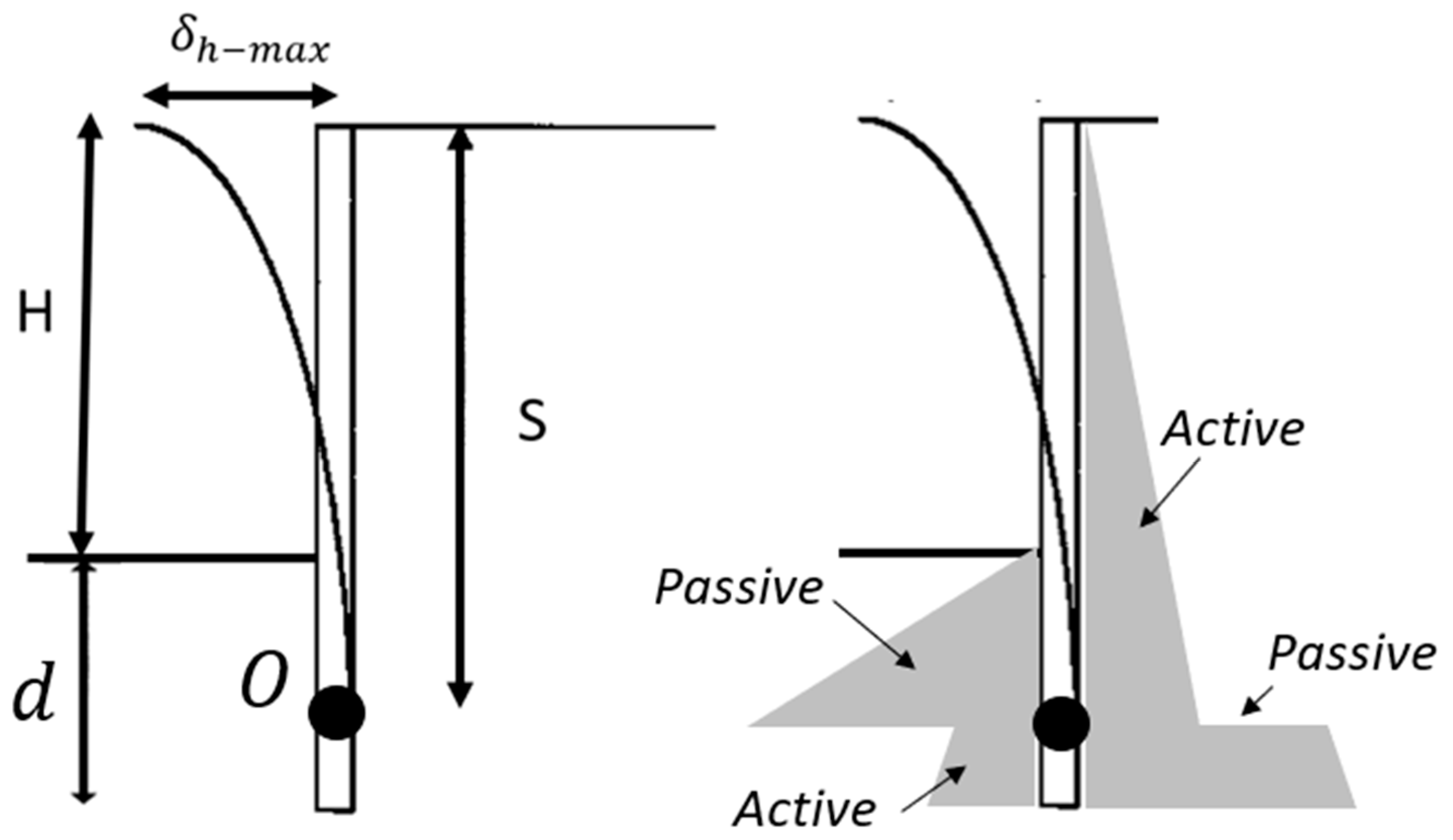
Figure 1 shows typical problem geometry and the active and passive lateral pressures for the cantilever problem. Accordingly,
H is the excavation depth,
O is the point of wall rotation,
d is the depth of wall embedment,
S is the distance from the top surface to the point
O, and
is the maximum wall displacement, which, for a cantilever wall, will occur at the top of the wall.
Limit equilibrium methods have since been refined according to empirical findings and integrated into building codes [
5]. However, limit equilibrium methods are limited to simple assumptions. Importantly, these methods cannot be used to compute wall displacements altogether. Embedded walls are increasingly applied in dense urban environments, where predicting displacements is crucial for avoiding damage to nearby structures due to excessive ground movement, underscoring a significant gap in traditional methods.
Numerical methods have revolutionized the analysis and design of geotechnical structures [
6]. Numerical methods, such as the finite element method (FEM), account for soil–structure interaction and compute the resultant stresses, strains, and displacements accordingly. Hence, no a priori assumptions are required for the distribution of earth pressures. Numerical methods can be used to account for various scenarios, as well as for the incorporation of advanced soil constitutive models, such as the hardening soil model (HSM). Schanz et al. (1999) developed the framework for HSM and provided the mathematical formulation. Experience gained by others has shown that HSM can simulate soil behavior under complex stress paths [
7]. Total strains depend on a stiffness that varies with stress and is distinct for initial loading compared to subsequent unloading or reloading. Plastic strains are determined through a multi-surface yield criterion. The HSM assumes isotropic hardening, influenced by both the plastic shear and volumetric strains. It employs a non-associated flow rule for frictional hardening and an associated flow rule for cap hardening. Accordingly, the HSM thoroughly accounts for fundamental soil properties, including strain hardening and dilatancy, and differentiates between loading and unloading stiffness. These nuances enable the HSM to better predict the nonlinear stress-strain response of soils.
The traditional linear elastic–perfectly plastic Mohr–Coulomb (MC) material model is widely used due to its simplicity. However, for the problem of embedded walls, the MC model does not provide reliable wall displacement results, to the degree that such models often yield reversed lateral and vertical displacements at the top of the wall [
8]. This matter has been demonstrated in a comparative study of a benchmark problem of a deep excavation in Berlin sand [
9]. This study demonstrates the demonstrates the limitations of the MC model in accurately predicting the behavior of soil–structure interaction in complex geotechnical scenarios, highlighting the need for more advanced constitutive models like the HSM.
Owing to its complexity, the HSM requires assessing and calibrating many input parameters, which in turn require several laboratory and field tests. Indeed, many researchers have conducted rigorous tests to compare these with numerical modeling results (e.g., [
10,
11]. Depending on the project scope and stage, it is often the case that limited data are available for selecting proper input parameters for the HSM. Hence, establishing input parameters for specific geotechnical problems is still a difficult and time-consuming task.
Arguably, surveys answered by geotechnical engineers can provide a good assessment of the current state of practice of geotechnical design and identify knowledge gaps. Therefore, an industry survey was conducted where practicing geotechnical engineers were requested to answer the following question: “
What methods or techniques do you predominantly use for the design of embedded retaining walls in your projects?”. As listed in
Table 1, multiple choices were given, with the instruction to select all that apply.
Table 1 shows the percentage and counts for each response. Based on 33 responders, results suggest that diverse approaches are being employed in the industry, with an inclination towards more sophisticated, computer-aided design approaches. This reflects upon the industry’s adaptation to the rapid technological advancements. When used in conjunction, more straightforward methods contribute a reliable source for verifying that the results of advanced numerical methods are within reason. This claim is valid for analysis of internal wall forces used for structural design of the wall in compliance with civil engineering building codes. However, concerning earth-retaining wall displacements, simplified methods that rely on limit equilibrium and spring models cannot be used as a benchmark comparison. Therefore, comparison to empirical data is crucial. It is noted that the survey question is part of an ongoing industry survey, and full results and their analysis are planned to be published and discussed in the future.
This paper aims to bridge the gap between theory and practice by conducting a rigorous numerical investigation of embedded walls with the HSM and comparing results against empirical data. According to this comparison, the ranges of HSM parameters that best align with the field data are inferred. Arguably, this approach offers a valuable starting point for engineers who wish to model embedded walls with the HSM, particularly when faced with limited data availability. To achieve this, we devised an automated computational scheme so that a series of numerical model results are compared to actual wall movements from the extensive global database provided by Long (2001) [
12].
2. Assumptions and Methodology
As mentioned briefly in the Introduction section, the objective of this study was to conduct a comparative analysis between numerical modeling results of embedded retaining walls and empirical data. To effectively address this objective, our research focused on the problem of cantilever walls rather than deep excavations that require lateral supports. This decision was rooted in the principle of beginning with a simpler problem, as deep excavations with lateral supports involve additional phenomena and inputs. Furthermore, the initial phase of many deep excavation projects is identical to cantilever wall scenarios, rendering the classical cantilever wall problem a good starting point for future investigations that include more complex geotechnical conditions.
The predictive power of numerical simulations is limited by the database they have been calibrated against [
13]. As discussed by [
14], large databases often exhibit biases stemming from their data collection process. Therefore, to properly conduct and interpret a numerical study, a deep understanding of the database used for empirical data is crucial.
The Long (2001) [
12] Database, hereinafter referred to as LDB, which the current analysis relies on, adopts a generalist approach. Accordingly, data are collected from worldwide locations rather than focusing on a limited geological formation with distinct characteristics. The approach adopted for the LDB allows for the identification of general trends. In turn, the LDB allows engineers to gain an intuition for the range of anticipated wall movements. The soils in LDB include residual soils, sands, gravel, and stiff clays, with soil shear strength ranging from weak to strong soils. Previous research has shown that the wall type (e.g., pile wall, diaphragm wall, etc.) has no notable impact on wall displacements [
15].
The wall displacements in LDB are normalized according to the excavation depth, i.e.,
is some percentage of
, as defined in
Figure 1. The results in LDP are somewhat surprising, as they show that
values were confined within a relatively narrow band of 0–0.5%, and an average of about 0.35%. Another interesting finding is that displacements were smaller than assumed by simplified and more traditional analysis methods. This finding has an important implication for cost-effective wall design, as data suggest that less stiff walls should perform adequately in many instances, rendering worldwide design practice overly conservative.
As discussed by Long (2001) [
12], analysis of the LDB implies that wall movements are relatively small in most cases. To replicate empirical data more realistically, we selected the small-strain hardening soil model (SS-HSM) for the modelling process. Alongside the HSM, SS-HSM has emerged as a significant advancement in geotechnical numerical modelling. The SS-HSM is an extension of the traditional HSM, which can capture nonlinear behaviour under small strains. Small strains are common in many geotechnical problems [
11]. Accordingly, SS-HSM is especially relevant in the case of embedded walls, where the majority of walls exhibit both small strains and nonlinear behaviour. The improved accuracy of SS-HSM does not come without a price, as this material model requires mode input parameters compared to the standard HSM. However, as the objective of the current paper was to establish general guidelines for initial parameter selection when in situ data are scarce, these additional inputs did not bear a significant limitation.
For the numerical modelling, the commercial finite element (FE) code RS2 was used [
16]. For typical embedded wall projects, plane strain conditions apply, rendering 2D models acceptable. Note that for basement excavations, where the excavation width and length are relatively similar, a 3D model is recommended for both a more realistic and cost-effective design [
6]. In our FE models, the embedded wall was simulated via line (or beam) elements. Line elements are zero-thickness elements, which efficiently capture wall axial, shear, and bending forces. Given the zero-thickness of the elements, the end-bearing resistance of the wall was not accounted for. To compensate for this, a lateral spring element was added to the base of the wall, thus realistically transferring vertical loads to the soil elements beneath the wall.
To model the interface between the wall and soil, special joint elements were assigned on both sides of the wall. The joint boundary stiffness is a numerical construct that simulates relative slip within an FE mesh. There are no definitive guidelines for accurately assessing the normal and shear stiffness values, which should be calibrated for each analysis [
17]. Additionally, a slip failure criterion was applied to the joint elements. The friction angle for this failure criterion can be estimated using empirical guidelines, and is typically assumed to be in the range of 0.6–0.8 of the soil internal friction angle [
4]. Similarly to the subdivision of data in LDB, no distinction was made between differences in soil layers and a homogeneous soil medium was assigned for all FE models.
To enhance the simulation process, we applied an automated computational scheme so that a series of models were generated with varying SS-HSM input parameters. In addition, other properties that were varied were the joint slip friction angle, the wall stiffness, and excavation and embedment depths. To establish the range of material properties of SS-HSM for the automated scheme, a comprehensive review was conducted, including [
11,
18,
19,
20]. On this basis, ranges and rules were established for generating a variation of input parameters. The models were then computed, and results were compared to LDP.
Table 1 lists the varied input parameters and their respective ranges. In this table, various inputs are varied directly, while other inputs are varied according to some assumption, as detailed in the table. For example,
, the unloading modulus, is known to be significantly larger than
, and was, therefore, assigned a value increased by a factor of 2–7. The relationship between the shear modulus
and
was also limited to a range of 1.1–1.7 [
19]. External Python codes were written for the automated generation of the models and their subsequent analysis. A detailed review of the technical data for the numerical models and the computational scheme is given in the following section.
3. Numerical Investigation
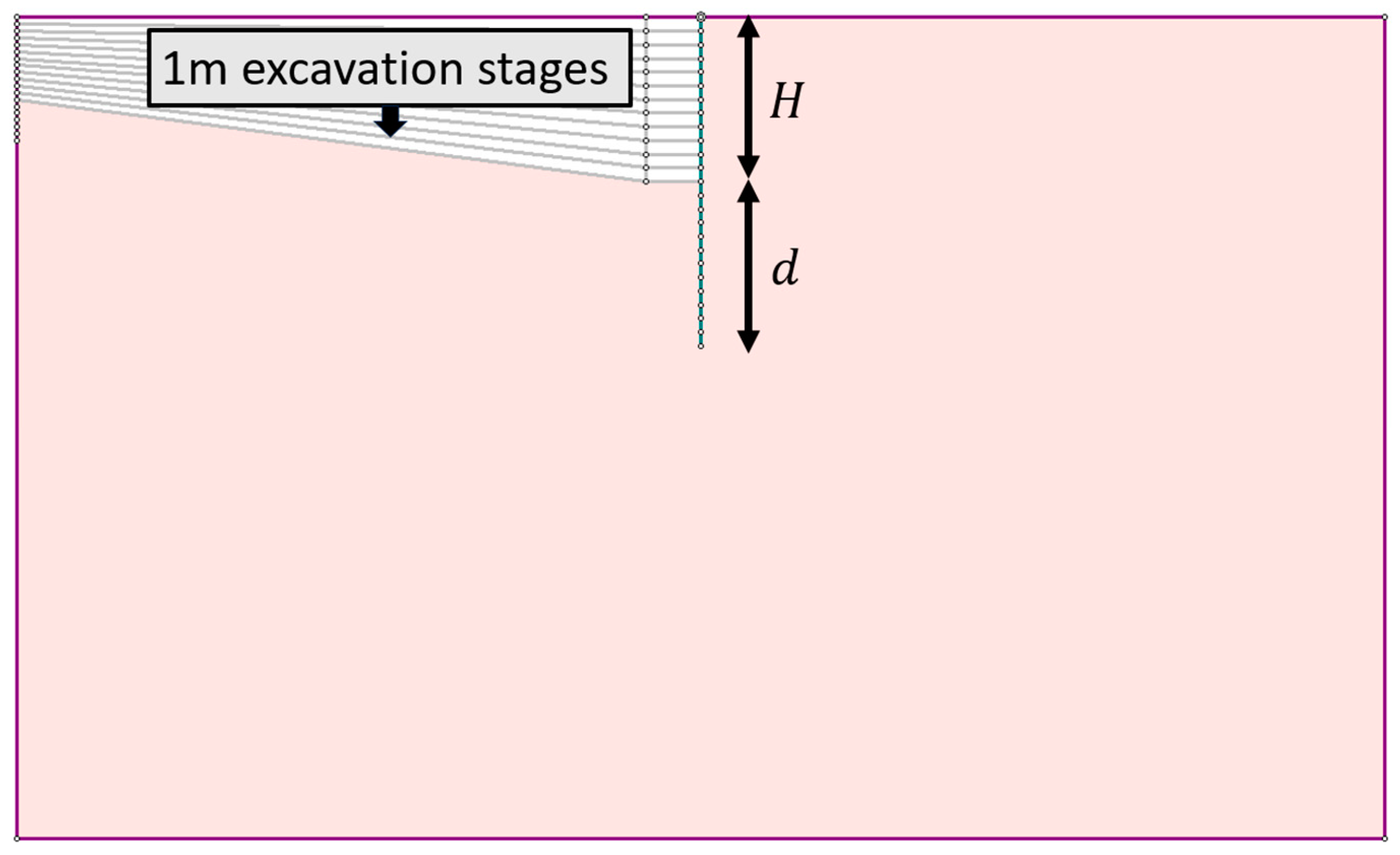
To conduct a systematic investigation, a basic geometric configuration was defined according to typical engineering scenarios, as shown in
Figure 2. The geometry was determined according to two primary variables: (1) the excavation height H and (2) the wall embedment depth d. To limit the geometric variation and focus on the impact of the SS-HSM parameters, these two dimensions were set equal for all models, i.e., H = d, assumed to be sufficient for typical conditions. The height H varied from 3–8 m with 1 m increments.
The excavation process in all models was divided into stages, where the ground level was lowered by 1 m in each stage. This staged approach allowed for a detailed analysis of the soil–structure interaction, where element yielding gradually progresses. Before the excavation stages, two initial stages were assigned for each model, the first for application of the in situ geostatic stresses, and the second for the installation of the wall. The lower excavation level was moderately sloped, as shown in
Figure 2. The angle of this slope was set to be lower than the friction angle, preventing additional and unwanted slope failure mechanisms that could erroneously impact results. On the other hand, it is argued that adding a slope is more realistic than a full removal of the entire portion of the lower level, as this could introduce unrealistic effects.
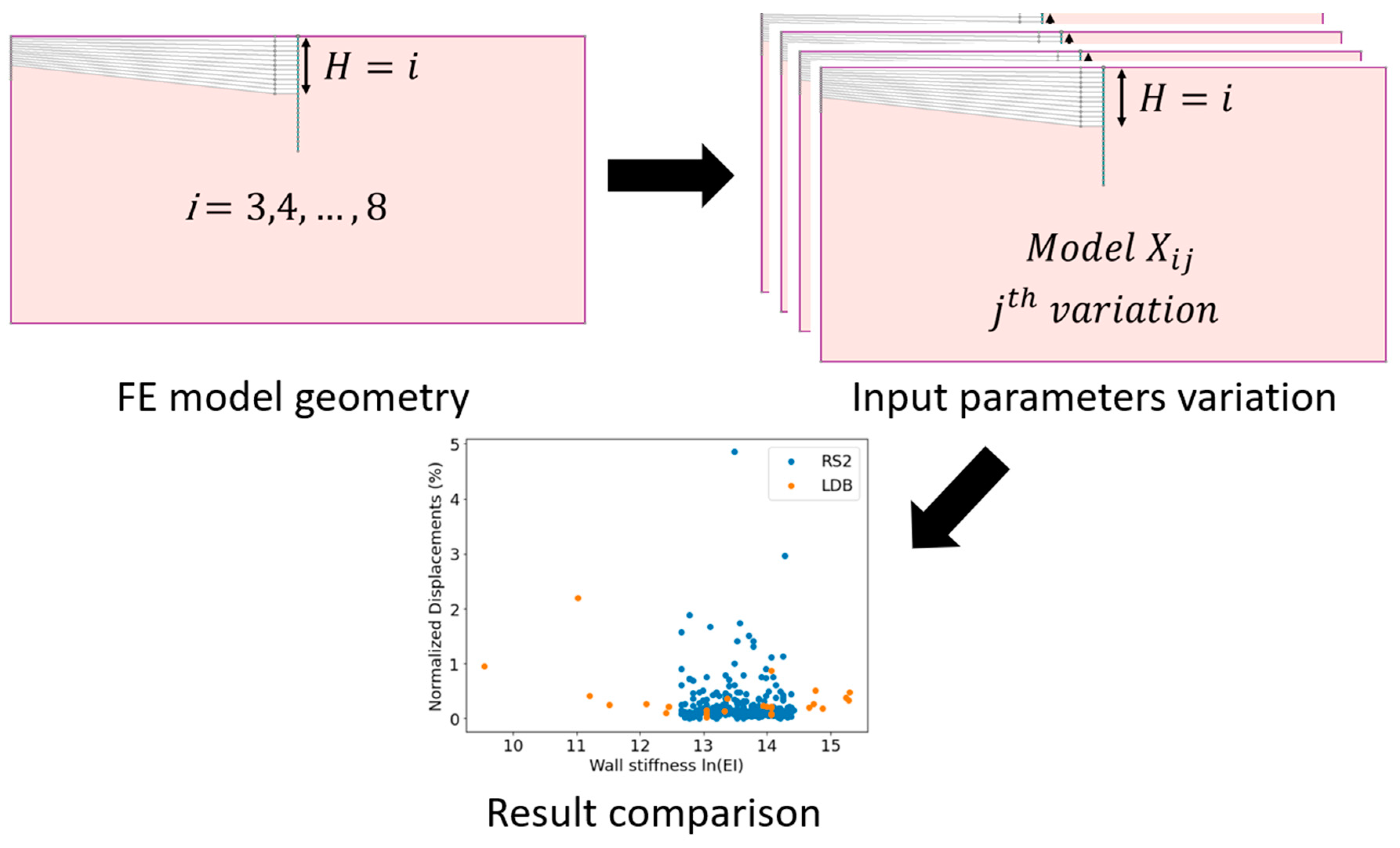
Figure 3 shows the flowchart for the computational scheme to automate the numerical investigation. Before automation, the initial six models were built and tested manually. Manual checking is particularly important in the face of advanced computational tools rapidly becoming more powerful. With insufficient human learning at the preliminary stages of modeling, there is a greater risk for the garbage-in-garbage-out phenomenon [
13].
Two Python scripts were written for the automation process, corresponding to the two arrows shown in
Figure 3. The first script interfaces with the FE model files by manipulating baseline models. Within this process, a total of six baseline models that correspond to the variation in height (i.e., H = 3, 4, …, 8) were created. A Monte Carlo scheme replaced the original input parameters from the baseline files, according to
Table 2. This process assigns input parameter values a random value according to a uniform distribution. It is acknowledged that the variation of geological materials regularly follows a normal distribution [
21]. For probabilistic analysis, where modelling aims to estimate the distribution of outcomes, assigning a normal distribution to parameters is fundamental. However, for the current analysis, the objective was to capture the range of results and compare this to the LDB. Given that the LDB itself consists of 26 case studies, it lacks the statistical significance for a more rigorous comparison. Another reason to generate evenly distributed inputs is for applying ML tools to interpret the numerical results. ML models perform better when trained on evenly distributed data [
22].
Accordingly, the input parameters were randomly generated 50 times for each baseline model (i.e.,
according to the notation shown in
Figure 3). Considering that there were six baseline models, a total of 300 FE models were created. The script arranges the input parameters from the models as a matrix. Using standard hardware, computer solving time for these 300 models could range between several hours and a few days, rendering the proposed modeling methodology feasible for practical purposes.
The second Python script (represented by the second arrow in
Figure 3) extracts the main results of the numerical models and arranges them as a column vector. Additionally, two important checks are applied within the script: (1) non-converging models are identified and (2) the displacement profile is checked for acceptability. The first check is crucial for detecting potential erroneous results due to numerical issues and loss of wall stability [
16]. The second check is applied to identify erroneous reversed displacements, typical for MC-based FE models [
23], as discussed in the Introduction section.
Finally, the results were compared to the actual displacements from the LDB. For this purpose, two plots devised by Long (2001) [
12] were reproduced. The vertical axis for both these plots is the normalized wall displacements, i.e.,
(see
Figure 1). The horizontal axes for the plots are the excavation height and the wall stiffness. The wall stiffness is represented by the expression
, where
is the concrete Young’s modulus, and
is the wall’s second moment of area. For all models, the
was kept constant and equal to 30,000 MPa, and
was calculated according to
, where
t is the varied wall thickness. The concrete unit weight and Poisson ratio were kept constant and assigned the typical values of 25 KN/m
3 and 0.2, respectively. This comparative analysis aimed to assess the simulation results’ reliability by examining their statistical alignment with empirically observed displacement patterns.
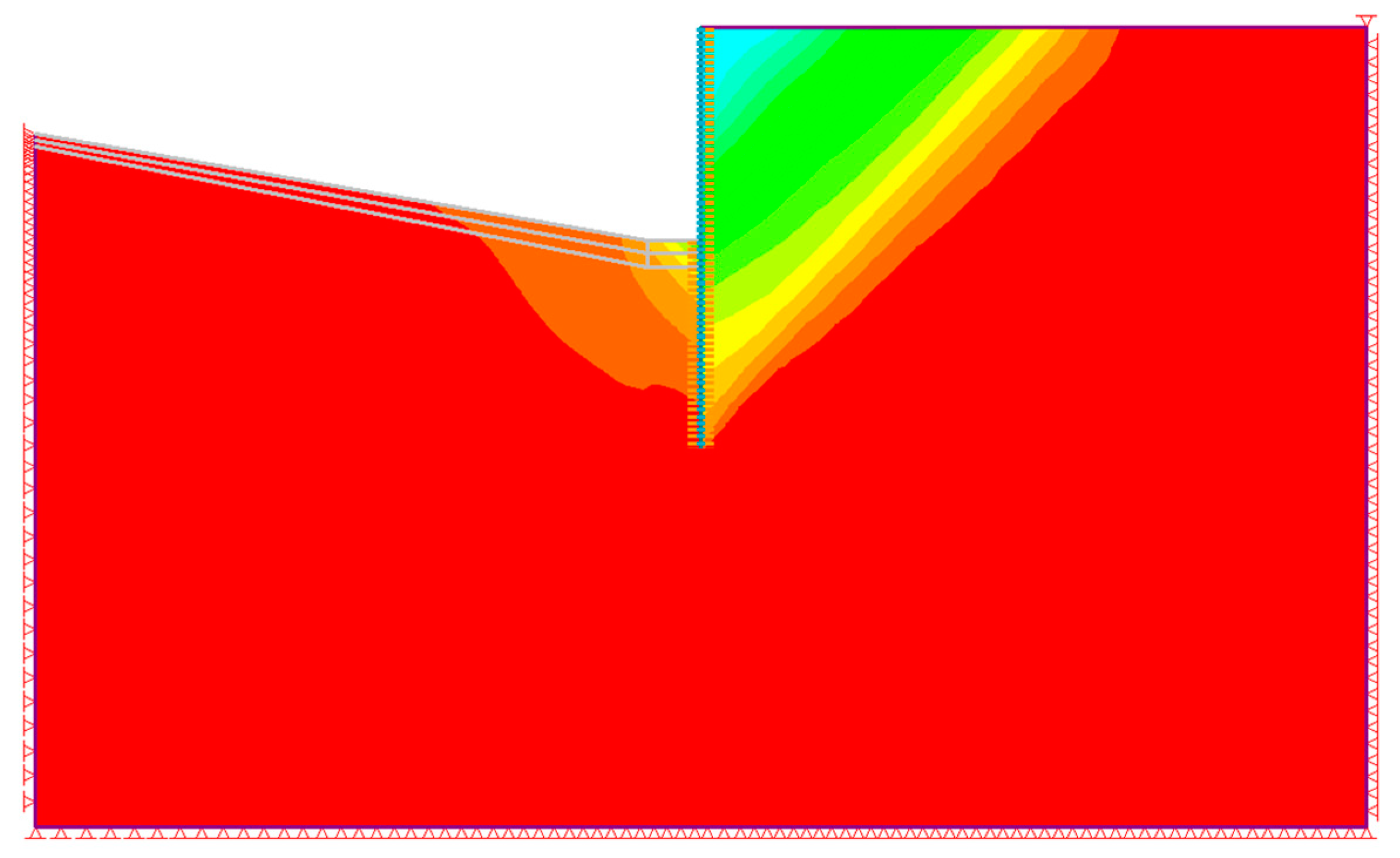
Regarding the general settings for the FE models, for SS-HSM in RS2, experience has shown that model performance is sensitive to stress analysis settings. Primarily, these settings influence the imitation of nonlinear behaviour using linear steps. Accordingly, the model tolerance was set to 0.001, the number of load steps was set to adaptive, the initial load increment was set to 0.0001, and the maximum load step was equal to 0.25. For the FE mesh, six-noded triangle elements were used, and elements as fine as 0.25 m were assigned to the zone of influence, i.e., the vicinity of the wall. Each model consisted of 10,251 elements at the initial stage before excavation. Model boundaries were set to 30 × 50 m, which extended beyond excavation-induced displacements. This can be observed in the horizontal displacement contours of an example model shown in
Figure 4. The bottom and lateral boundaries are fully restrained. The numerical investigation results and their comparison to the LDB are presented in the following section.
4. Results and Discussion
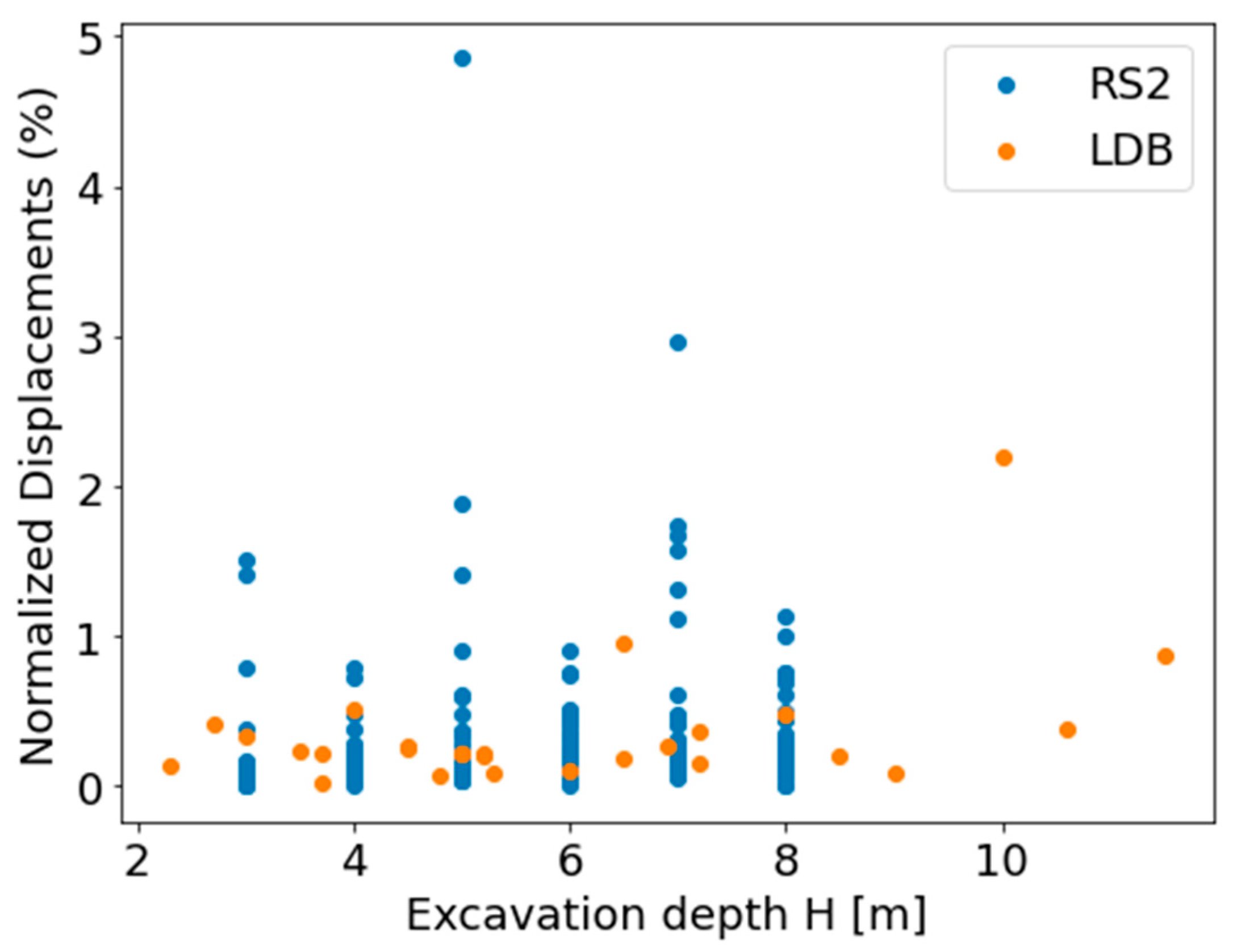
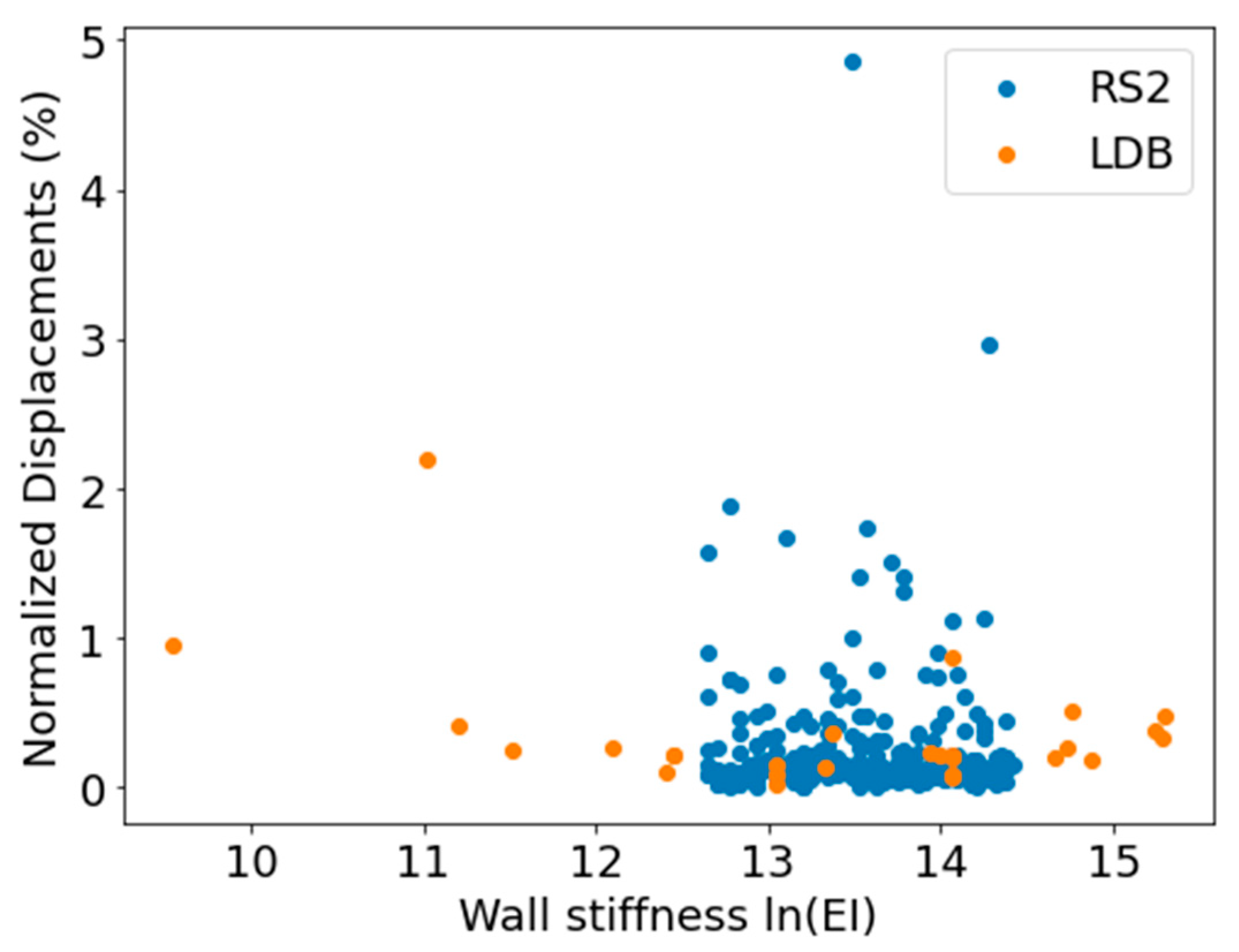
In total, 300 models were computed via the RS2 solver, which allows for automated computation of numerous models. It was found that only four numerical models failed to converge, and these models were, therefore, disregarded. None of the models yielded reversed displacements. The numerical data, thus consisting of 296 results of normalized wall displacements, were plotted alongside the LDB, as shown in
Figure 5 and
Figure 6. Based on a visual comparison of the data, empirical and numerical results are in good agreement, as the vast majority of datapoints are concentrated within a narrow bandwidth of 0–1%, with several outlier results. Also, similarly to the LDB findings, numerical results are independent of excavation depth and wall stiffness.
For a more rigorous comparison, a basic statistical analysis was applied. The average of the normalized displacements of the LDB is 0.35%, whereas the numerical results yielded a lower mean value of 0.21%. The quartile distribution of the numerical results shows that 25% of the values are below 0.046%, 50% (median) are below 0.11%, and 75% are below 0.18%. These results indicate that a significant portion of the data are concentrated at lower displacement values, similarly to the LDB. The empirical data and numerical results have a similar standard deviation of 0.42 and 0.43, respectively. Thus, the numerical investigation results generally prove that the RS2 models with the SS-HSM material model successfully replicate embedded wall behavior.
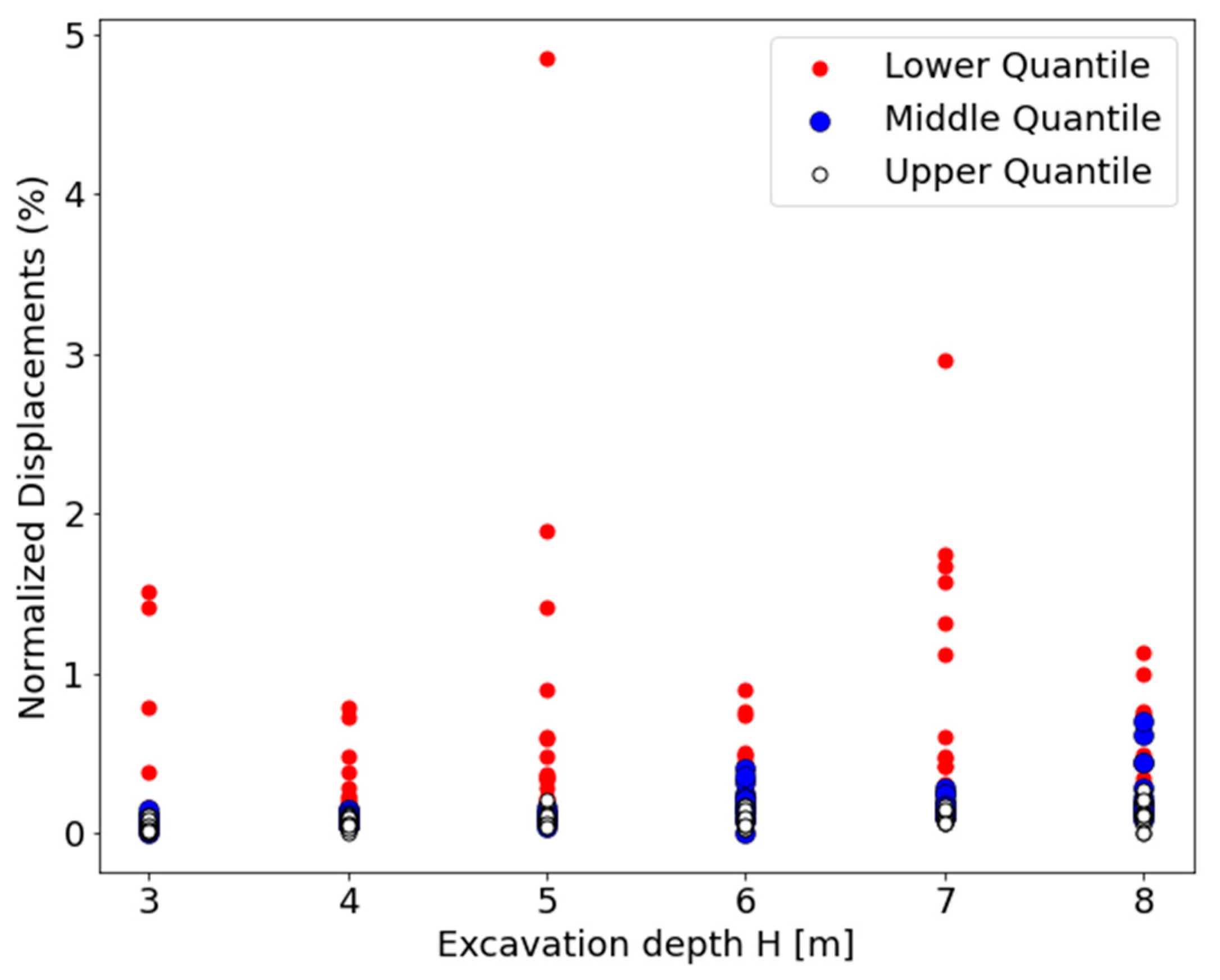
To augment the interpretation of the numerical data, we computed feature importance, a data analysis tool from machine learning (ML). Coupling ML tools with numerical analysis has been shown to accelerate back-analysis tasks and assistance in other modelling tasks [
24]. Feature importance analysis shows the impact of each varied input parameter on the desired outcomes, thus providing insight into which inputs require greater attention. The computational method for feature importance was first derived by [
25]. To compute feature importance, a proper ML model must first be built. Accordingly, the input parameters from the numerical models were arranged as an X matrix, and the resultant normalized displacements were defined as a corresponding Y-column vector. The open-source Scikit-learn library was imported into Python for ML analysis. A comprehensive review of ML applications and the Sci-kit learn library is given by [
25].
The random forest regression model was implemented using functions from this library. The correlation between the X and Y data was low, such that R2 < 0.5. The coefficient of determination R2 provides a straightforward assessment of the ML model performance; a result of one indicates perfect accuracy, and zero indicates no correlation. The interpretation of this low correlation is not conclusive and could stem from several issues. A greater number of models is likely required, as the SS-HSM consists of many input parameters with highly nonlinear results. In this context, it should be noted that the fact that both the empirical data and numerical results are not evenly distributed but consist of small wall movements with few large outliers renders such datasets difficult to train accurately [
26].
Due to the low performance of the random forest model, feature importance results should be treated with caution [
24]. Nevertheless, whether feature importance results are meaningful can be tested, as hereby described. Feature importance was computed using the built-in function in the Sci-Kit library [
25]. The results showed that the displacements are predominantly dictated by the SS-HSM three Young’s moduli (i.e., E_ref50, E_oed, and E_ur), while the impact of the other parameters importance is secondary.
Accordingly,
Figure 7 shows a modified plot of the data, where the numerical results were divided into three even quantiles: upper, middle, and lower quantile. The quantiles correspond to the Young’s moduli ranges listed in
Table 2. Note that the Young’s moduli are dependent on each other and roughly proportional, as defined in
Table 2. Observing
Figure 7, it can be identified that the Young’s moduli quantile largely predicts the magnitude of normalized wall displacement. Thus, the results of the feature importance are confirmed. This finding could assist others in faster calibrating their embedded wall models, as displacement results can be controlled by adjusting the SS-HSM Young’s moduli parameters.
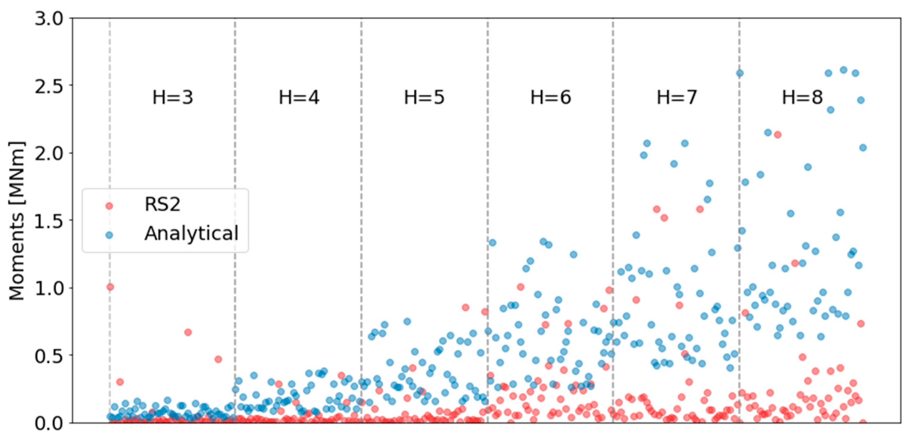
As discussed in the Introduction section, under the current state of practice, traditional analytical limit equilibrium methods are frequently being used for embedded wall design. The design process involves computing the internal forces and selecting the suitable cross-section, as well as the steel reinforcement for concrete walls. For each of the 300 models, we computed the maximum internal bending moment using simple analytical analysis of active and passive forces based on the soil internal friction angle, based on simple lateral earth pressure theory. For these computations, soil cohesion was disregarded. Note that this simplification is assumed to be negligible, as the cohesion values assigned to the FE models lie within a very low range of 0–0.1 MPa (see
Table 2). Safety factors were not applied to the analytical calculation, in order to allow for a valid comparison.
Figure 8 shows these results juxtaposed alongside the SS-HSM FE model results obtained from RS2. The results are divided according to the wall heights. As can be observed, the bending moments from the analytical calculations are larger, and increase with wall height. This discrepancy can be primarily attributed to the FE models’ more accurate representation of soil–structure interaction, which takes into account the soil’s stiffness in resisting movement—a factor overlooked in simpler analytical approaches. This finding is in line with the observation reported by Long [
12], that design practices based on analytical methods are overly conservative.
5. Summary and Conclusions
Embedded walls are ubiquitous geotechnical structures and accurate prediction of wall displacements remains a significant engineering challenge. Simplified methods, such as lateral pressure theory, do not provide displacement results, and FE analyses with the Mohr–Coulomb material model have been shown to fall short of yielding realistic displacement results. In this regard, the SS-HSM model has generally demonstrated promising results for various geotechnical applications but requires the knowledge of multiple input parameters.
This paper presents an extensive numerical investigation of embedded walls to systematically compare FE modelling results with a database of actual wall movements. For this purpose, an automated computational scheme was developed, and the power of computer automation was employed. Through this process, a large number of models were computed according to varied SS-HSM input parameters, as well as other parameters, such as wall thickness and soil–wall interface.
The SS-HSM input parameter variation was established according to research by others, as well as practical experience gained by the authors. The results of the comparative study demonstrate that the numerical results are in close agreement with empirical data. For both, the majority of results are confined within small, normalized displacements, and the statistical distribution is similar. Hence, it is argued that the ranges of SS-HSM input parameters assumed for this paper, as listed in
Table 2, can be used as a good starting point for others who wish to simulate embedded walls. The three Young’s modulus parameters for the SS-HSM have been found to impact displacement results significantly. Thus, proper assessment of these parameters is crucial for obtaining realistic predictions.
Additionally, our analysis shows that the FE models align more closely with actual embedded wall behavior, potentially leading to less conservative, yet realistic, design outcomes compared to traditional analytical methods. This observation complements our primary findings by highlighting the advantage of advanced FE modeling in capturing complex geotechnical behaviors.
It is essential to acknowledge the limitations of the current work. The models are limited to several simplifying assumptions. Consequently, predictions for specific cases should be made with caution and subject to thorough review, as the consequences of wall failure can be catastrophic. Additionally, only the simplest case of a cantilever wall was analyzed; therefore, further investigation is required for deep and sequenced excavations, which involve additional geotechnical phenomena.


