Study on the Prediction of Slope Failure and Early Warning Thresholds Based on Model Tests

Abstract

In recent years, slope failure caused by heavy rainfall from linear precipitation bands has occurred frequently, causing extensive damage. Predicting slope failure is an important and necessary issue. A method used to predict the time of failure has been proposed, which focuses on the tertiary stage of the creep theory, shown as V = A/(t_r − t), where V is the velocity of displacement, A is a constant, and (t_r − t) is the time until failure. To verify this method, indoor model experiments and field monitoring were used to observe the behavior of surface displacement. Seven cases of laboratory experiments were conducted by changing the conditions in the model, such as materials, the thickness of the surface layer, and relative density. Then, two cases of field monitoring slope failure were examined using this method. The results show that, in the tertiary stage of creep theory, the relationship between tilt angle velocity and the time until failure can be expressed as an inversely proportional relationship. When the tilt angle velocity has reached the tertiary creep stage, it initially ranges from 0.01°/h to 0.1°/h; when near failure, it was found to be over 0.1°/h, so, combining this with previous research results, this is a reasonable value as a guideline for an early warning threshold.

1. Introduction

Landslides triggered by rainfall occur globally and have significant impacts on lives, property, infrastructure, and the environment, for example, in North and South America [1,2], Europe [3,4], and Asia [5,6]. For this reason, early warning systems aim to mitigate the risk of landslides and are indeed garnering attention as a non-structural, cost-effective countermeasure to landslide disasters. Consequently, the development of technology that can accurately detect the precursors of a landslide has become a significant issue.

Rainfall thresholds are used in many early warning applications to issue warnings when monitored rainfall exceeds a predefined level [7,8,9,10,11]. Rainfall is indeed widely and easily monitored by both meteorological institutions and various private sectors. However, the occurrence of sediment disasters is not only related to rainfall intensity but also influenced by local soil conditions, the gradient of the slope, and geohydrological factors. Therefore, for high-accuracy early warning, measuring local surface displacement is necessary. Surface displacement’s role in early warning systems for landslide detection has been a subject of research for a considerable period. Past literature has shown that various techniques have been employed to monitor surface displacement by installing different measurement methods. For example, regarding local field measurements, some researchers suggest that, by measuring the surface strain levels of slopes, it is possible to forecast slope failure in earlier years [12,13,14,15]. Recently, tilt sensors that measure the tilt angle of the surface layer have been developed and are being widely used [16]. In terms of large-area measurements, remote-sensing techniques are other tools for monitoring ground surface displacement. Techniques like radar [17,18,19], light detection and ranging (LiDAR) [20], and global navigation satellite systems (GNSS) including the Global Positioning System (GPS) [21] have been used to measure signatures associated with natural hazards such as landslides and slope failures.

Local field measurement is an effective approach for early warning systems because it is low-cost and easy to install the sensor on the ground surface. By measuring the surface displacement, it can predict the time of failure using a method based on the creep behavior of soil. The creep model is shown in Figure 1.

Saito (1969) [14] has demonstrated a linear relationship between the strain rate in the secondary creep region and the time until collapse, as shown in Equation (1). They suggest that this relationship continues for a long time even when it enters the tertiary creep region from the secondary creep region, and propose the following equation, which establishes an inverse relationship between strain rate and the remaining time until collapse.

$$\log t_r\mathrm{’}=2.33-0.916\log \left(\dot{\epsilon }\times {10}^4\right)\pm 0.59$$

(1)

where $t_r\mathrm{’}$ is time until collapse (min) and $\dot{\epsilon }$ is the steady strain rate.

Fukuzono (1985) [15] pioneered a novel approach for forecasting the time of failure, known as the inverse velocity method. This method was formulated by integrating the relationship of the velocity of surface displacement just before failure (Equation (2)). Owing to its simplicity and ease of use, it has become the most widely used prediction method based on displacement.

$$\frac{1}{v}={\left\{a\left(\alpha -1\right)\right\}}^{\frac{1}{\alpha -1}}\cdot {\left(t_r-t\right)}^{\frac{1}{\alpha -1}}$$

(2)

where v is the velocity of the slope surface displacement, t is the current time, t_r is the estimated time to failure, a and α is constant.

Equations (1) and (2) have good performance for traditional ground extensometers, which capture linear displacements when cracks occur in slopes. Recently, tilt sensors that measure the tilt angle of the ground surface layer have been developed and are being used [16]. Tilt sensors are becoming popular because they are not only easier to install than ground extensometers but also can be monitored at multiple points in real time.

However, it is not easy to set the threshold for issuing early warnings. In this study, the main purpose is to find a practical method that can be used to support the application of tilt sensors. Focusing on the tertiary stage of the creep model, a simple method predicting the surface failure of slope is proposed. To verify this method, serval cases of laboratory experiments were conducted changing the conditions in the model, such as the material, the thickness of the surface layer, and relative density. Two cases of field monitoring of slope failure were examined using this method and the threshold for early warnings.

2. Current State of Early Warning Systems

2.1. Proposed Method

When a landslide or slope failure event takes place, the process of deformation normally follows the creep model under the main condition of constant stress, as shown in Figure 1a. Initially, the distortion progresses notably, but subsequently diminishes gradually, a phenomenon referred to as primary creep. Following primary creep, the deformation continues at a consistent pace, known as secondary creep. Eventually, the deformation rate experiences an exponential increase, ultimately resulting in collapse and landslide, which is termed tertiary creep. Using Equation (2), let α = 2, and, from the method of Fukuzono (1985) [15], a new Equation (3) is as follows:

$$V=\frac{\mathrm{A}}{\left(t_r-t\right)}$$

(3)

where V is the velocity of displacement, A is constant, and (t_r − t) is time until failure. It can be considered that the material at each measured point on the slope is different. Furthermore, each measured point can have a constant A. This material behavior is known as the Monkman–Grant relationship, as mentioned in [22]. Equation (3) is an inverse proportional relationship, also known as an inverse variation or inverse proportionality, which is a mathematical relationship between two variables. If one variable increases, the other decreases proportionally, and vice versa.

The behavior of Equation (3) during a landslide is explained in Figure 1b. During the secondary creep phase, the deformation undergoes gradual advancement at a consistent velocity, resulting in the inverse velocities remaining relatively constant. During the tertiary creep stage, there is an exponential increase in displacement, and the reciprocal of velocity tends to decrease linearly. Hence, the transition from the secondary to the tertiary creep stage can be estimated by analyzing the reciprocal of the velocity. A sample soil creep result for the laboratory experiment is shown in Figure 2.

2.2. Warning Criteria for Slope Failure

It is effective to monitor using observation equipment on slopes where there is risk of a landslide or where signs of a landslide have been detected. The conventional ground extensometer is commonly employed to measure local changes within a limited region. This device utilizes an invar line that is positioned over a crack and can detect linear alterations. On the other hand, the tilt sensor is utilized to monitor the tilt angle of the surface layer. By strategically positioning numerous tilt sensors along the slope, it becomes possible to catch planar variations as well. In the process of risk assessment and mitigation using monitoring technologies, specific criteria for evaluating landslides have been established for ground extensometers and tilt sensors. These criteria serve as guidelines for making judgments on the measured results.

However, it is important to note that these criteria are primarily designed to assess changes occurring on a daily or monthly basis. From the perspective of emergency response and safety monitoring at construction sites, it is essential to detect and understand changes that occur at shorter time intervals quickly and effectively. This entails establishing thresholds as benchmarks for actions such as evacuation, which are determined by real-time monitoring of changes every hour. Uchimura (2015) [16] has proposed a warning stage for slope collapse based on the distribution trend of the relationship between the remaining time until collapse (time until re-stabilization) and the velocity of the tilt angle. This proposal pertains to the tilt sensor, which has garnered significant attention in recent times, albeit still being in the research stage. Threshold ①: An alert should be triggered if the value is above 0.01° per hour. Threshold ②: If the rate is above 0.1° per hour, a precautionary alert is issued.

Given the aforementioned information presented in Figure 1, it can be inferred that the tilt angle of the surface layer exhibits a consistent rate of acceleration during the secondary creep phase. However, in the event of a collapse, the rate of acceleration experiences a sudden and exponential surge during the tertiary creep phase. Hence, to prompt a timely reaction to slope collapse, it is deemed efficacious to give an advance notification when deformation advances and transitions into tertiary creep.

3. Laboratory Experiment

To understand the behavior of soil creep, two kinds of indoor model experiments have been conducted.

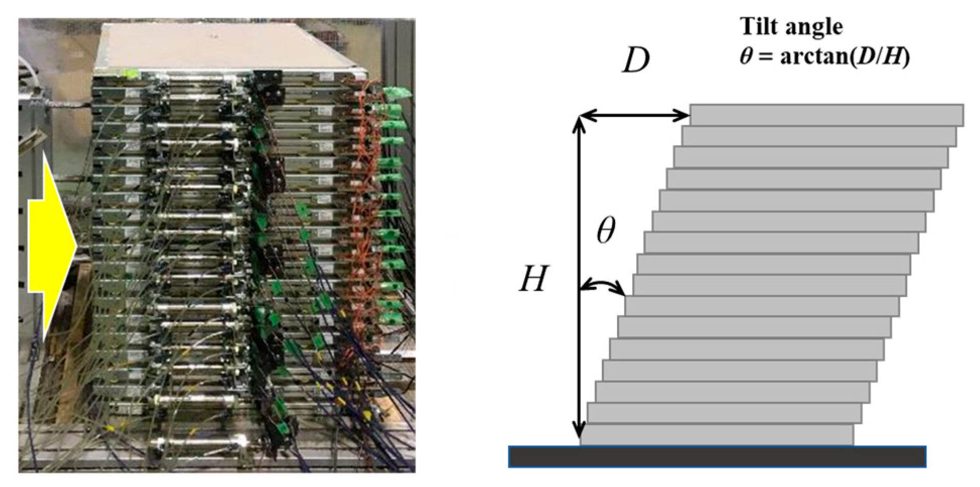
3.1. Laboratory Experiment Apparatus

The study employed a multi-layer shear box apparatus to replicate the forces experienced in a slope, enabling the measurement of displacements and forces within each layer (see Figure 3). The specific aspects of the multi-shear model are described in detail in reference [23]. The physical model can comprise a maximum of 20 frames, with each frame having a height of 0.05 m, a length of 0.6 m, and a width of 0.54 m. Every individual frame is equipped with wheels to reduce the amount of friction that occurs between the steel frame and its surroundings. Air cylinders are utilized to apply a consistent horizontal load on each layer, thereby replicating the shear force associated with the inclination angle. Load cells and displacement sensors are installed at each stratum as well. The precipitation water permeates the upper stratum and exits through the lower portion of the model, under the influence of an artificially induced rainfall intensity of 60 mm/h.

To replicate the failure of the slip surface, direct shear tests were also carried out. Two layers make up the test; each has a 0.035 m height, 0.31 m length, and 0.21 m breadth. The upper layer applies a vertical load, while a constant horizontal force is applied by air cylinders. Water is infiltrated into the soil through ceramic disks located at the bottom (see Figure 4).

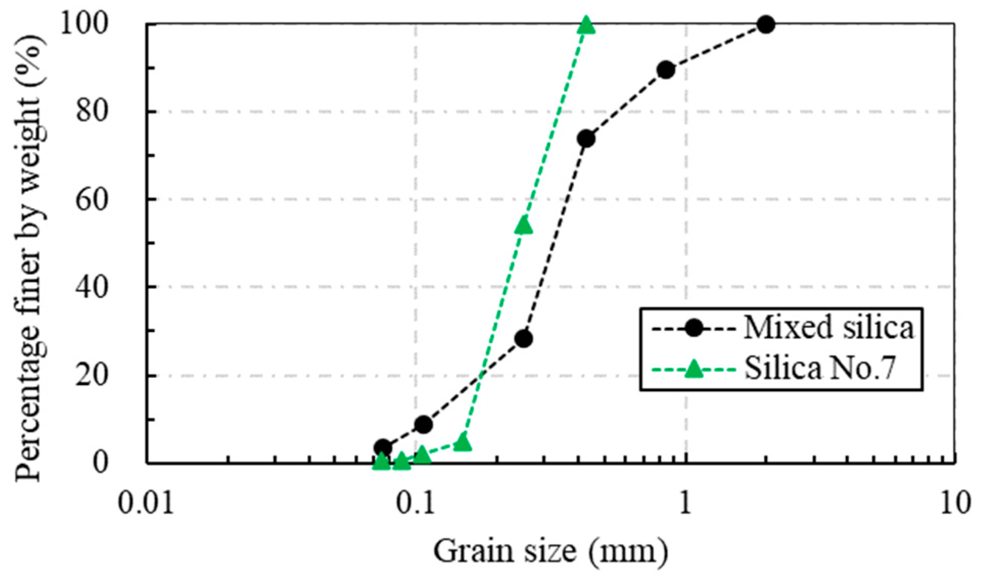
3.2. Soil Characterization

This study utilized two distinct materials to conduct laboratory experiments. The initial mixture consisted of silica sand No. 4, No. 5, No. 7, and No. 8, combined in the proportion 1:1:3:1. The second material under consideration was Silica No. 7.

Table 1. Main geotechnical properties of the studied soil.

Parameters	Mixed Sand	Silica No. 7
Dry density (ρd) (g/cm3)	1.48	1.34
Strength parameters (Φ)	43.90	37.10
Strength parameters (kPa)	7.40	28.60
Initial volumetric water content (%)	7	7

displays the characteristics of the soil, whereas Figure 5 illustrates the particle size distribution curve.

3.3. Experimental Cases

To simulate the behavior of surface displacement, seven cases of laboratory experiments were conducted by changing conditions such as the material, thickness of the surface layer, and relative density. The following

Table 2. Multi-layer model experiment cases.

Case	Layers	Material	Relative Density (Dr)
1	20	Mixed sand	50%
2	10	Mixed sand	50%
3	20	Silica No. 7	70%
4	20	Silica No. 7	50%
5	10	Mixed sand	50%

and

Table 3. Direct shear test experiment cases. The material is mixed sand.

Case	Vertical Pressure	Horizontal Pressure	Water Injection Pressure
6	8.40 kPa	7.60 kPa	0.15 kPa
7	8.40 kPa	8.60 kPa	0.15 kPa

show the details. Cases 1–5 used a multi-layer model where the rainfall intensity was 60 mm/h. Case 1 and Case 2 used the same material and relative density but varied the height of the layer. Case 3 and Case 4 used the same material and layer height but varied the relative density. Case 1 and Case 4 used the same layer height and varied the material. Cases 6–7 used the direct shear test; Case 6 and Case 7 used the same material, vertical load, and water injection pressure, but varied the horizontal load.

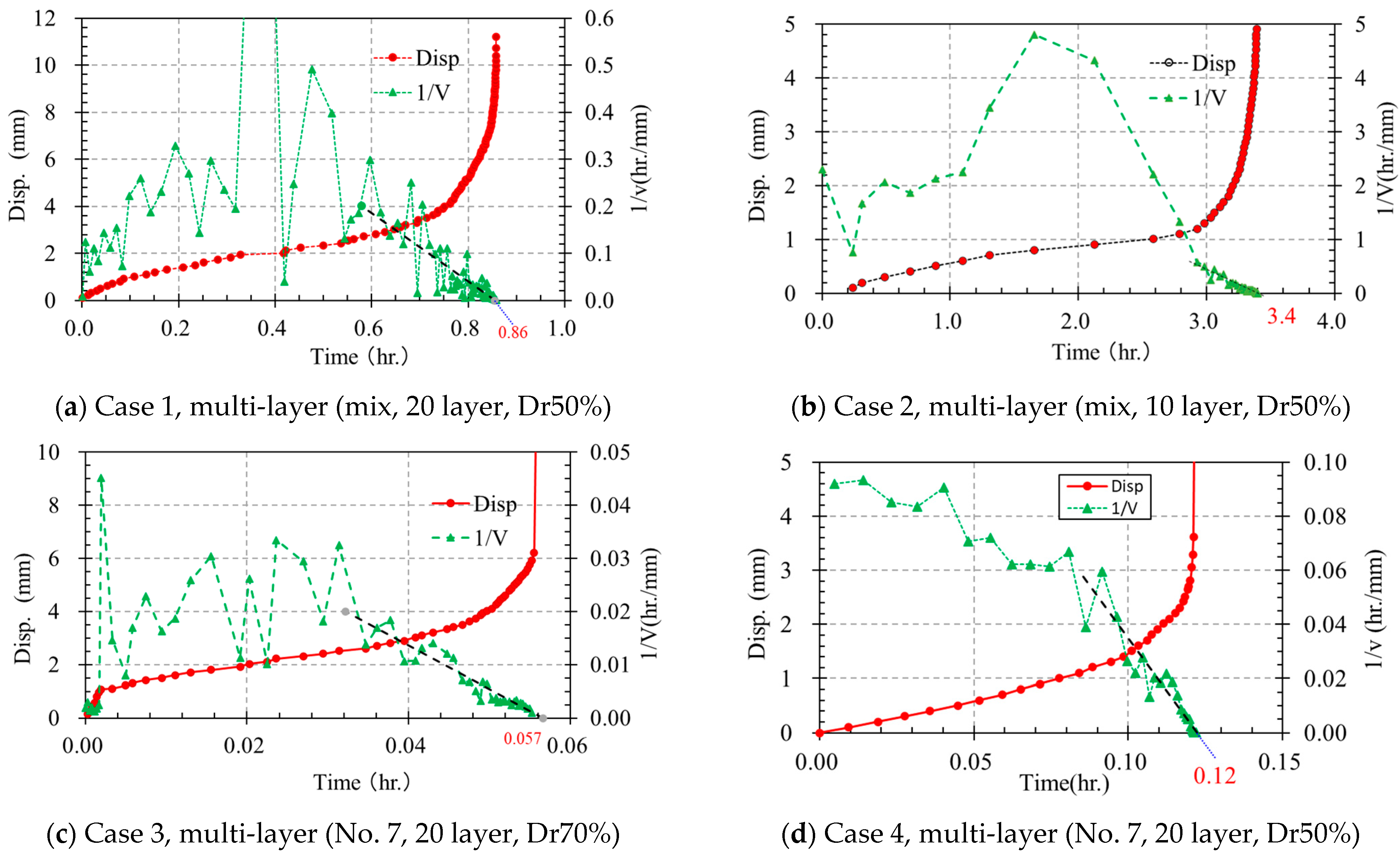
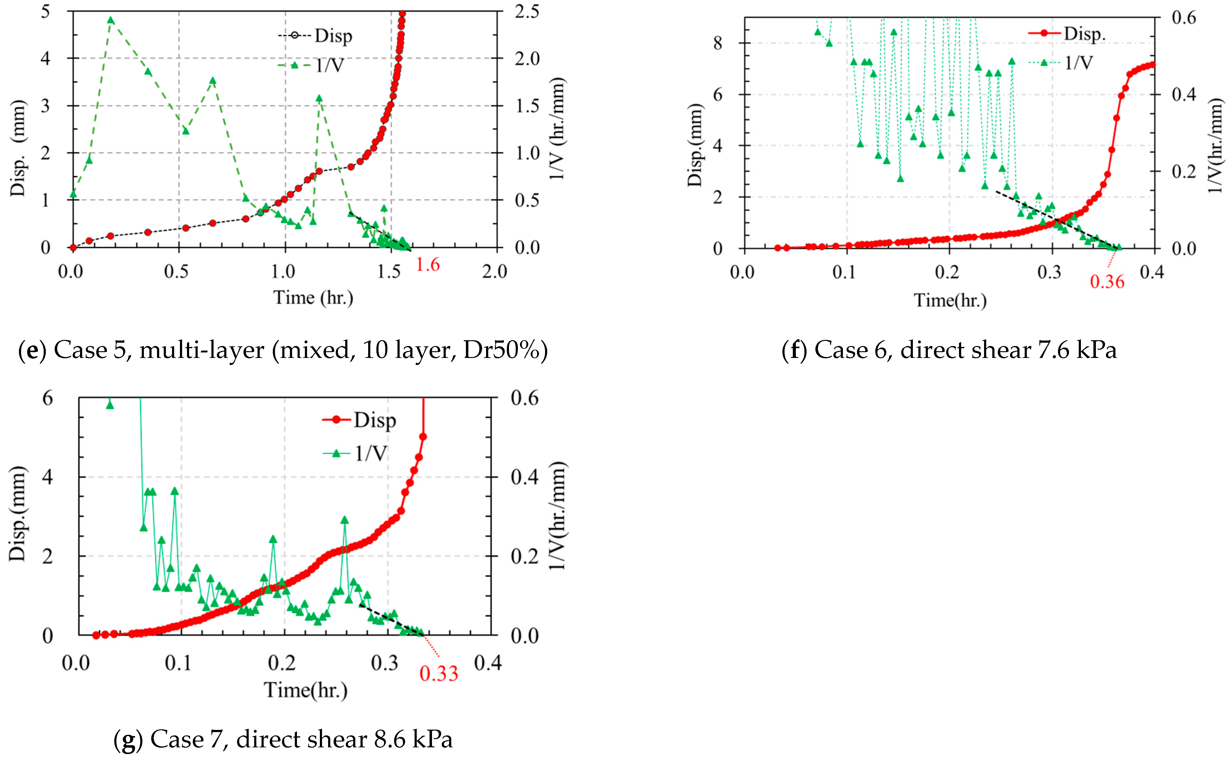
3.4. Experimental Results

To verify the method expressed by Equation (3), several cases of laboratory experiments were conducted by changing the conditions of the model, such as the materials, the thickness of the surface layer, and relative density.

The results of the laboratory experiments under different conditions are summarized in Figure 6. The temporal change in displacement is represented by the red dotted line in every case, while the green dotted line represents the temporal change in the inverse velocity. The black dotted line shows the linear change in the tertiary stage, and the intersection with the X-axis is the predicted time.

According to the inverse velocity in Case 1, when it begins to decrease from 0.5 h, it indicates the start of the tertiary creep stage. It then accelerates from 0.6 h and ultimately fails at 0.86 h, as shown in Figure 6a.

In Case 2, the tertiary creep stage starts at 2.8 h, accelerates from 3.0 h, and finally fails at 3.4 h, as seen in Figure 6b.

In Case 3, the tertiary creep stage starts from 0.036 h and ultimately fails at 0.057 h, as depicted in Figure 6c.

In Case 4, the tertiary creep stage begins at 0.09 h and fails at 0.12 h, as illustrated in Figure 6d.

In Case 5, the tertiary creep stage commences at 1.4 h and concludes with failure at 1.6 h, as presented in Figure 6e.

In Case 6, the tertiary creep stage initiates at 2.8 h and finally fails at 3.6 h, as demonstrated in Figure 6f.

Finally, in Case 7, the tertiary creep stage starts at 0.28 h and fails at 0.33 h, as shown in Figure 6g.

The logarithmic relationship between time until failure and velocity is shown in Figure 7. This logarithmic relationship can be used to calculate the constant value of the parameter α, which is mentioned in Equation (2). The parameter α of each case is mainly determined by the data at the tertiary stage. Every case results in a different value.

In the cases for the multi-layer model, the parameters α are 2.49, 2.33, 2.08, 1.87, and 1.64 respectively, corresponding to cases 1, 2, 3, 4, and 5. In the direct shear test experiment, the parameters α are 2.01 and 2.11, respectively, corresponding to cases 6 and 7.

Finally, all seven cases are summarized in Figure 7h. This shows that the average value of the parameter α is 2.

Table 4. Multi-layer experiment cases.

Case	Predicted Failure Time	Real Failure Time	Accuracy Ratio	α
1	0.79	0.86	0.92	2.49
2	3.40	3.41	0.99	2.33
3	0.05	0.06	0.91	2.08
4	0.12	0.13	0.92	1.87
5	1.23	1.60	0.77	1.64
6	0.36	0.37	0.97	2.01
7	0.33	0.34	0.97	2.11

summarizes the results for predicted failure time, real failure time, accuracy rate, and the value of the parameter α.

The predicted failure time is calculated from inverse velocity and the intersection with the X-axis; all of them are shown in Figure 6. The real failure time is defined as when the displacement is over 8 mm.

The accuracy rate is calculated as the real failure time divided by the predicted failure time. The accuracy rates are in the range 0.77~0.99, and most of them are over 0.9. This shows that this method can provide a reasonably accurate prediction.

The value of α is from Figure 7. The value of α ranges from 1.87 to 2.49. The average α is 2.07; minus the decimal point, it is approximately equal to 2.

The average of α is 2.07.

3.5. Verification Using Indoor Experiment Results

Verification was conducted on the deformation speed during tertiary creep, similar to the results of field measurements using the multi-layer shear model test. The method of determining the slope angle from the displacements obtained in each layer with this device was calculated using the height from the bottom layer to the top layer and the cumulative displacement from the initial state of the top layer, as shown in Figure 8.

Case 1 and Case 2, as shown in Table 1, were used for analysis. The results of each experiment are shown in Figure 9, and the relationship between the slope angle speed during tertiary creep and the remaining time until collapse is shown in Figure 10.

The slope angle increased rapidly after 0.8 h for Case 1 and after 3 h for Case 2, leading to failure. Changes in the tilt angle rate and its reciprocal were observed after 0.6 h for Case 1 and after 2.7 h for Case 2, suggesting that they had reached the tertiary creep stage. In the tertiary creep interval, although Case 1 generally decreased linearly with some variation, Case 2 showed a two-stage slope similar to the site-A field measurement results, and differences in predicted collapse time were observed when approximating a straight line in each interval.

In terms of the relationship between time until failure and the tilt angle rate during tertiary creep, both Case 1 and Case 2 had a change gradient similar to the previous data in Figure 10 but were located below the distribution range. This is because the laboratory material is different from the site material; the phenomenon of the material’s behavior, called the Monkman–Grant relationship, is mentioned by [22], and may be useful in predicting the failure time from the observed creep deformation rate. The tilt angle rate is larger than the threshold of 0.1°/h for Case 1. A slight interval between the threshold at 0.01°/h and the threshold at 0.1°/h can be seen for Case 2.

4. Field Monitoring

As mentioned in previous studies, deformation progresses in an accelerated manner during tertiary creep and leads to collapse, both in laboratory experiments and on actual slopes. In this study, two cases confirmed the issuance timing of an early warning system that used microelectromechanical systems (MEMS) tilt sensors monitoring the ratio of the tilt of slopes in Japan. In these cases, tilt sensors were used to monitor the actual slopes, and the process leading to a collapse due to rainfall was documented.

4.1. Site A—Case on the Slope Beside the National Highway

The initial occurrence of slope collapse transpired adjacent to the roadway as a consequence of precipitation induced by Typhoon 11 during the period spanning 17 to 18 July, 2015. In this particular instance, a tilt sensor was positioned on 21 July with the primary objective of safeguarding the building of countermeasures. It successfully recorded the behavior leading up to the subsequent fall that transpired on 22 July.

The observed variation in tilt angle, as detected by the tilt sensor, is depicted in Figure 11. The angle of tilt underwent deformation for around six hours, starting at 20:00 on 21 July with a pace of 0.083° per hour. Subsequently, it experienced acceleration and reached a rate of 0.89° per hour at 8:00 a.m. on 22 July, continuing to distort for approximately four hours. Immediately before the occurrence of the collapse at 12:00, the rate of angular displacement experienced an acceleration, reaching a value of 12° per hour. Subsequently, at 12:30, structural failure transpired, resulting in the sensor’s descent.

Figure 12 illustrates the temporal variation in the rate of change of the tilt angle velocity, which is the combined angle in the X and Y directions, as well as its reciprocal, starting at 16:00 on 21 July. The rate of change in the tilt angle remains relatively stable until approximately 16 h later, with minor oscillations, after which it experiences a significant and rapid increase. The reciprocal of the phenomenon exhibits a degree of dispersion as a result of minor variations in the angle until approximately 16 h has elapsed. Subsequently, it can be reasonably approximated by a prominent two-stage slope, consisting of a segment denoted “a” and another section denoted “b”, which is further divided into concave forms according to Fukuhara’s formula. The estimated time of the collapse, determined by extrapolating the reciprocal extension line to the intersection point on the x-axis, is closely aligned with the actual measurement time, averaging 20.5 h after the initial 16 h mark. However, in a specific portion of the figure, the estimated collapse time occurred earlier than the actual measurement time, specifically after 17.2 h. Conversely, in the b section, the estimated collapse time occurred later than the actual measurement time, specifically after 22.4 h.

Figure 13 depicts a graphical representation illustrating the correlation between the rate of tilt angle change and the remaining time until collapse in the context of tertiary creep. The collapse time was specifically designated to occur after a duration of 20.5 h. Furthermore, it exhibited a comparable change gradient and demonstrated a tilt angle speed exceeding the threshold value of 0.1°/h during tertiary creep.

4.2. Site B—Case on the Slope Beside the National Highway

This case study presents an instance wherein the response of a valley fill embankment site to significant rainfall caused by Typhoon 24 in September 2018 was documented using an inclination sensor. The sensor captured the behavior of the site during the collapse event triggered by the intense precipitation.

Figure 14 depicts the recorded alterations in the inclination angle at the specified location. The inclination angle exhibits a gradual increase after 19:00 on 30 September, albeit at a sluggish pace, followed by a notable acceleration in its rate of growth after 22:00.

Figure 15 and Figure 16 depict the temporal evolution of the angular velocity (composite angle) and its reciprocal, commencing at 17:00 on 30 September. The rate of change of angular velocity experiences a rapid increase after a time period of 5.5 h. Conversely, the rate of change of the reciprocal of angular velocity exhibits a linear decline after a time period of 5 h, and it intersects with the x-axis roughly 6 h later.

The findings derived from Site B, as depicted in Figure 17, provide a summary of the correlation between the duration remaining until collapse during tertiary creep (with a presumed collapse time of 6.0 h) and the angular velocity of the slope, akin to the representation in Figure 13. Despite being located at the lower end of the distribution range, the change gradient remains consistent, with the slope angular velocity typically exhibiting a value of 0.1°/h or higher during tertiary creep.

5. Discussion

In this study, the experimental results were correlated with the creep mechanisms proposed by Saito (1969) [7] and Fukuzono (1985) [15]. Each of these provides a fundamental theoretical formula for predicting landslide failure times. A logical subsequent step would be to link these experimental results with theoretical analysis and utilize this connection to validate the reliability of early warning thresholds [12].

Fukuzono (1985) [15] proposed a method for predicting the failure time of a slope based on the inverse velocity of the slope surface, a term referred to as the prediction of failure time from surface displacement. This method is associated with the tertiary creep stage, as slope failure occurs at the final stage of this tertiary creep in the time-to-failure process. The predicted failure time is determined by extending a straight line that correlates with the gradient of inverse velocity until it intersects with the time axis. In the discussion of Figure 7, it was considered that the value of α can be set to 2. By setting the value of α to 2, based on the average results from the seven cases of laboratory experiments, Formula (4) can indeed be derived from Formula (3). This simplification could potentially make further calculations or theoretical analysis more manageable.

In Figure 10, the displacement in two laboratory experiment cases is converted to a tilt angle and compared with the results of previous research. Figure 13 and Figure 17 present results from two sites. These figures illustrate that tilting rates vary over time until slope failure occurs. This observation is based on a summary of several case history studies. It suggests that using the velocity of the tilt angle for early warning thresholds is both feasible and reasonable. One can envision quantifying this interpretation by employing Formula (4) to explicitly calculate the early warning threshold response from the velocity of the surface displacement or tilt angle. However, these are located below the distribution range. This is because the laboratory material differs from the site material. The phenomenon of the material’s behavior, known as the Monkman–Grant relationship, which is mentioned in [22], may be useful in predicting the failure time based on the observed creep deformation rate.

The velocity of the tilt angle, which is considered to have reached the tertiary creep stage when deformation progressively increases, ranges from 0.01°/h to 0.1°/h. It was found that many cases are over 0.1°/h. From these observations, it is considered that the following two-stage warning threshold proposed by Uchimura (2015) [16] is a reasonable value as a guideline for an early warning threshold:

Alert: When it exceeds 0.01°/h.

Early warning: When it exceeds 0.1°/h.

In summary, findings on the mechanisms of tertiary-stage creep in a serial laboratory model test and field measurements have been presented. Taking these processes together leads to an interpretation of the experimentally observed velocity and the time-of-failure behavior of creep.

6. Conclusions

A method was introduced to predict failure time by utilizing the relationship between the velocity of displacement and time until failure. Secondly, seven cases of laboratory experiments were conducted under varying model conditions, such as materials, the thickness of the surface layer, and relative density, to examine this method. Furthermore, the measured surface tilt angle data from two field monitoring cases on natural slopes were used to evaluate the validity of the results corresponding to the relationship between velocity and time until failure from the indoor laboratory experiment. Finally, the following conclusions were drawn from this study:

(1)

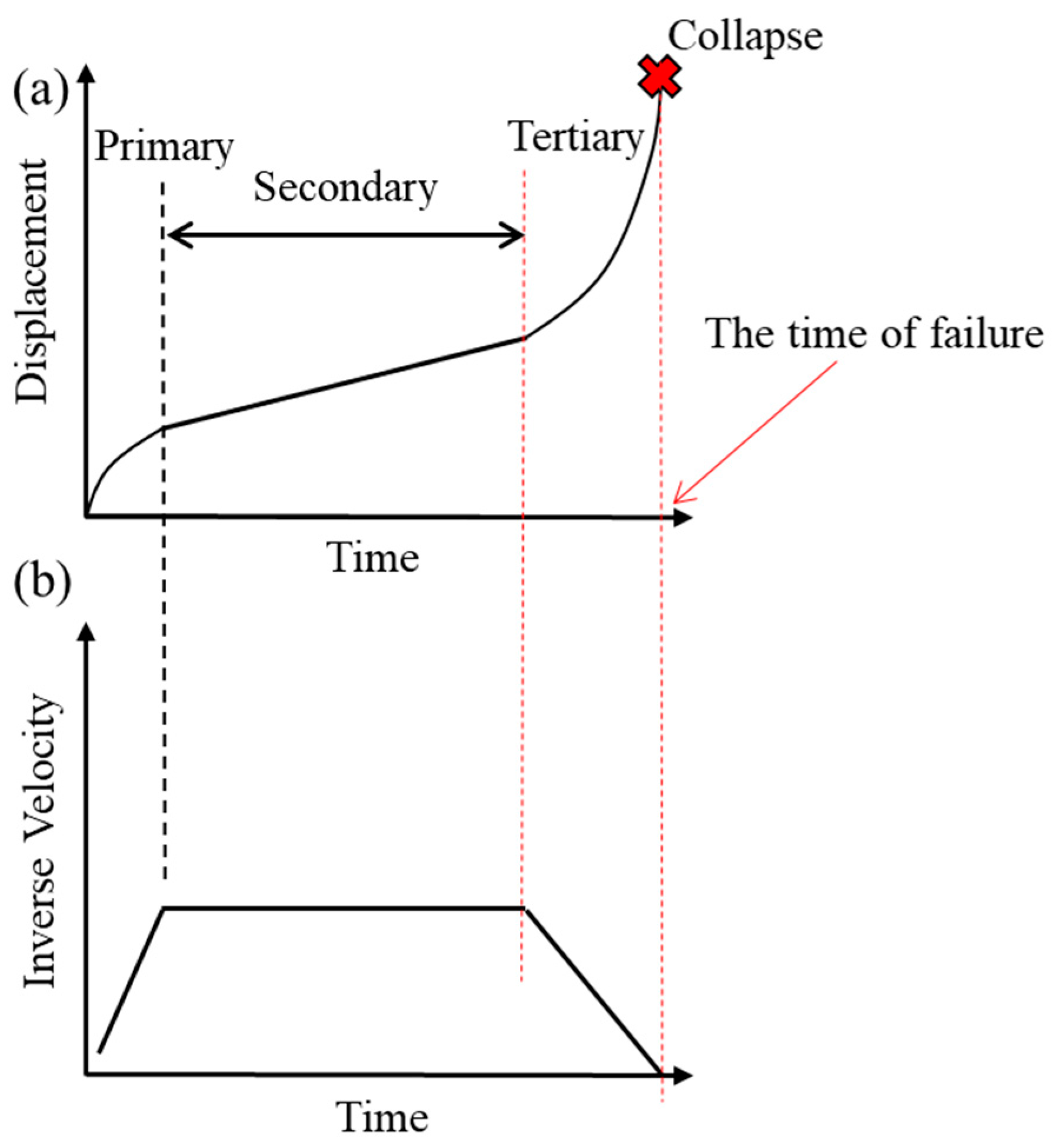
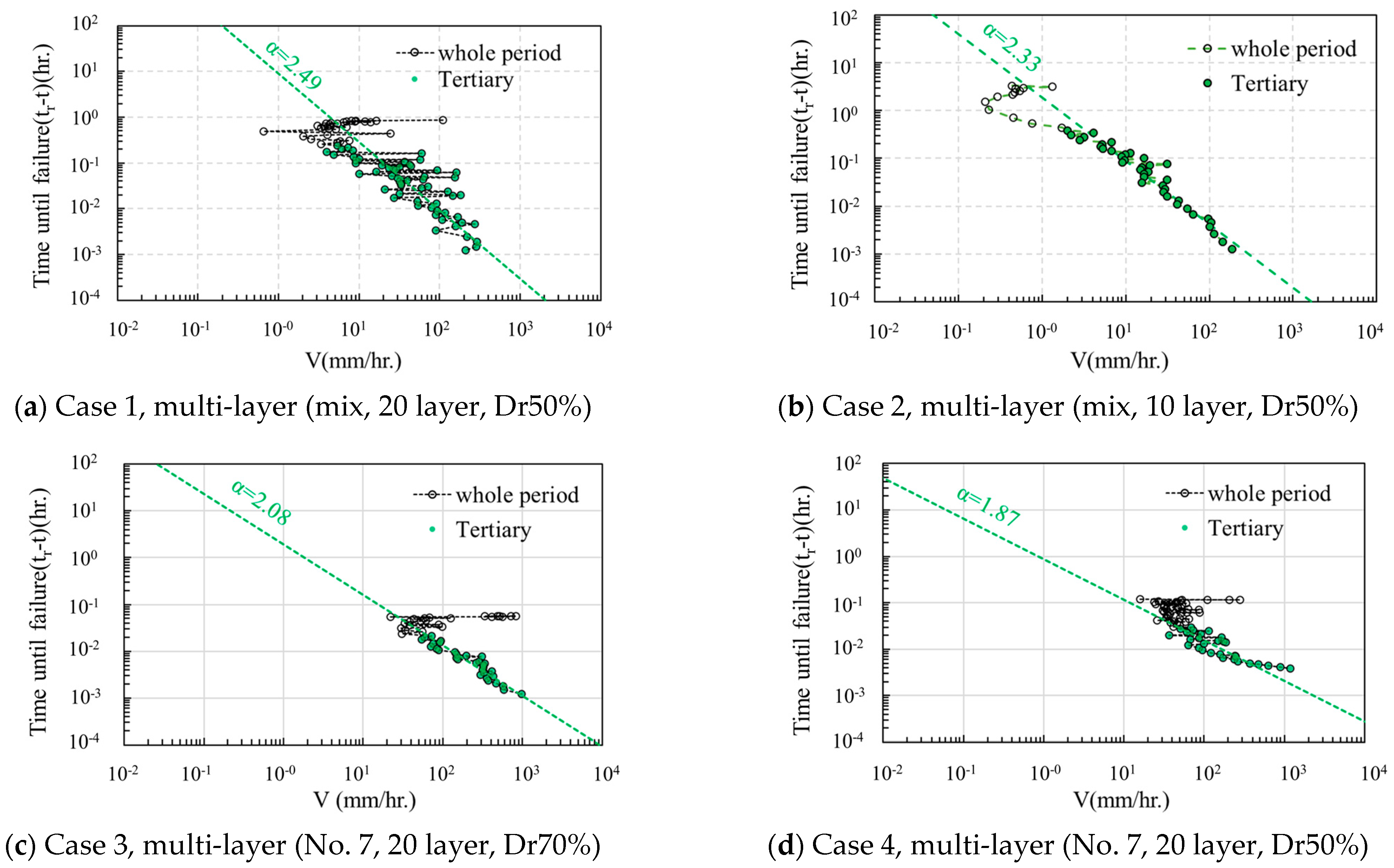
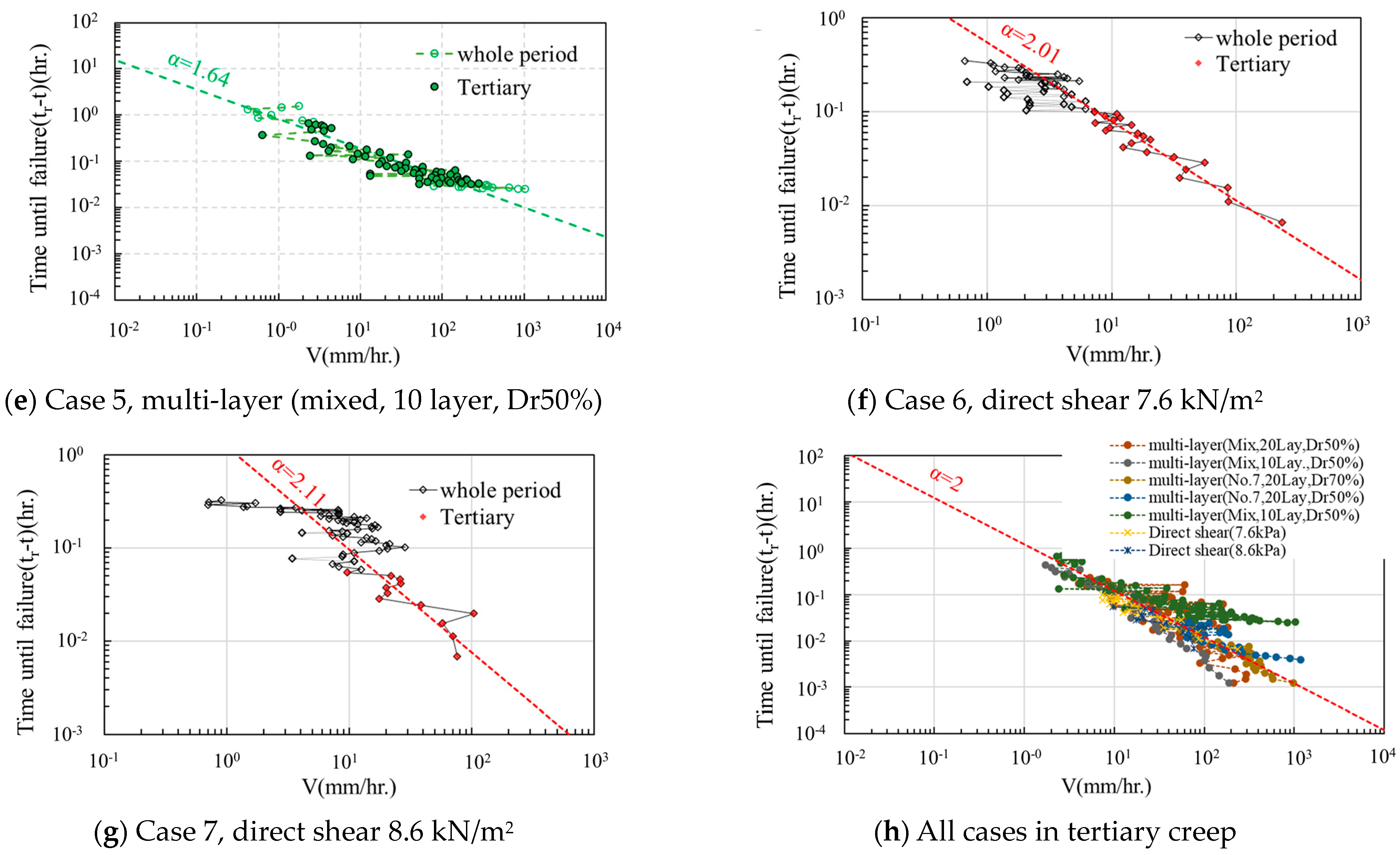
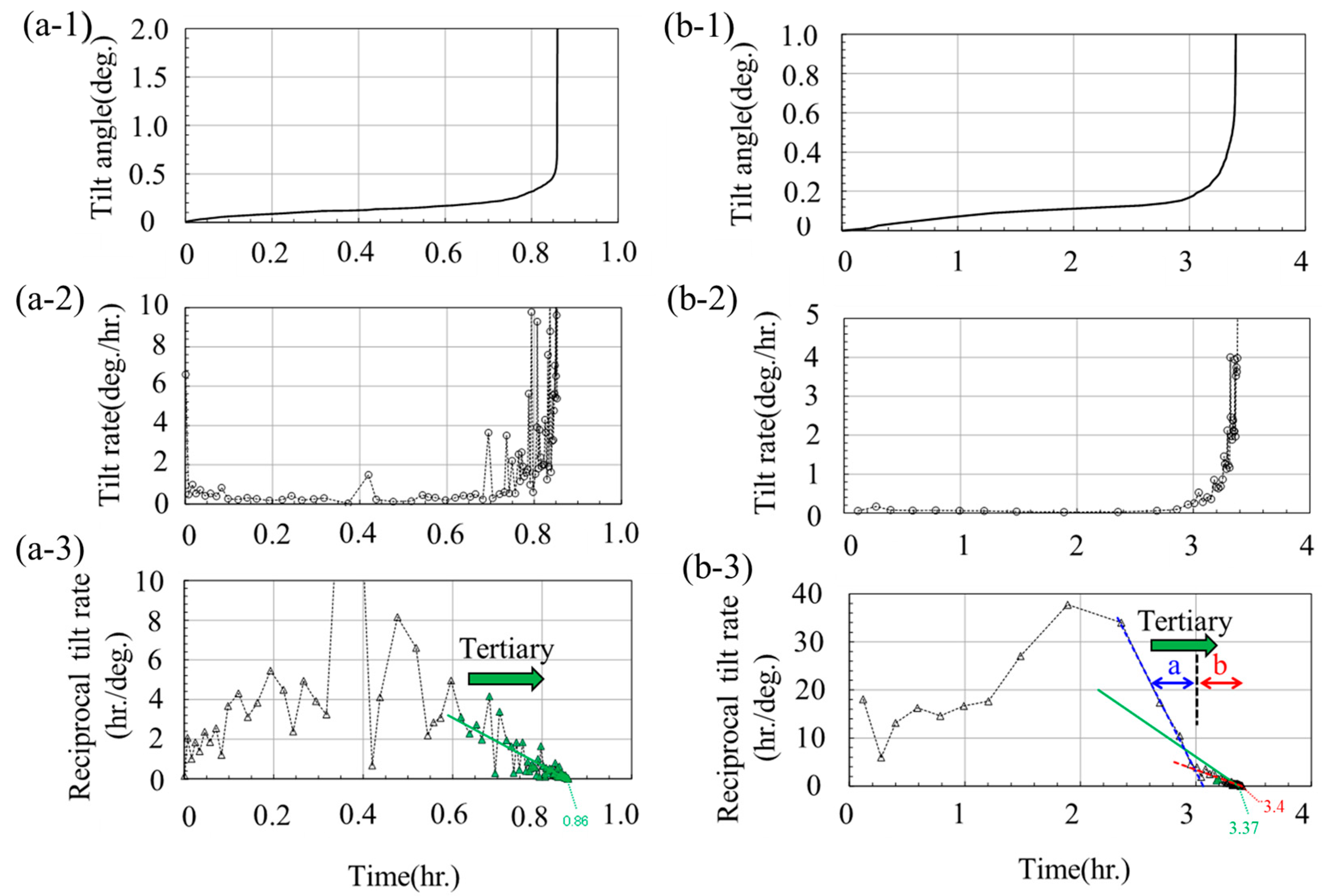
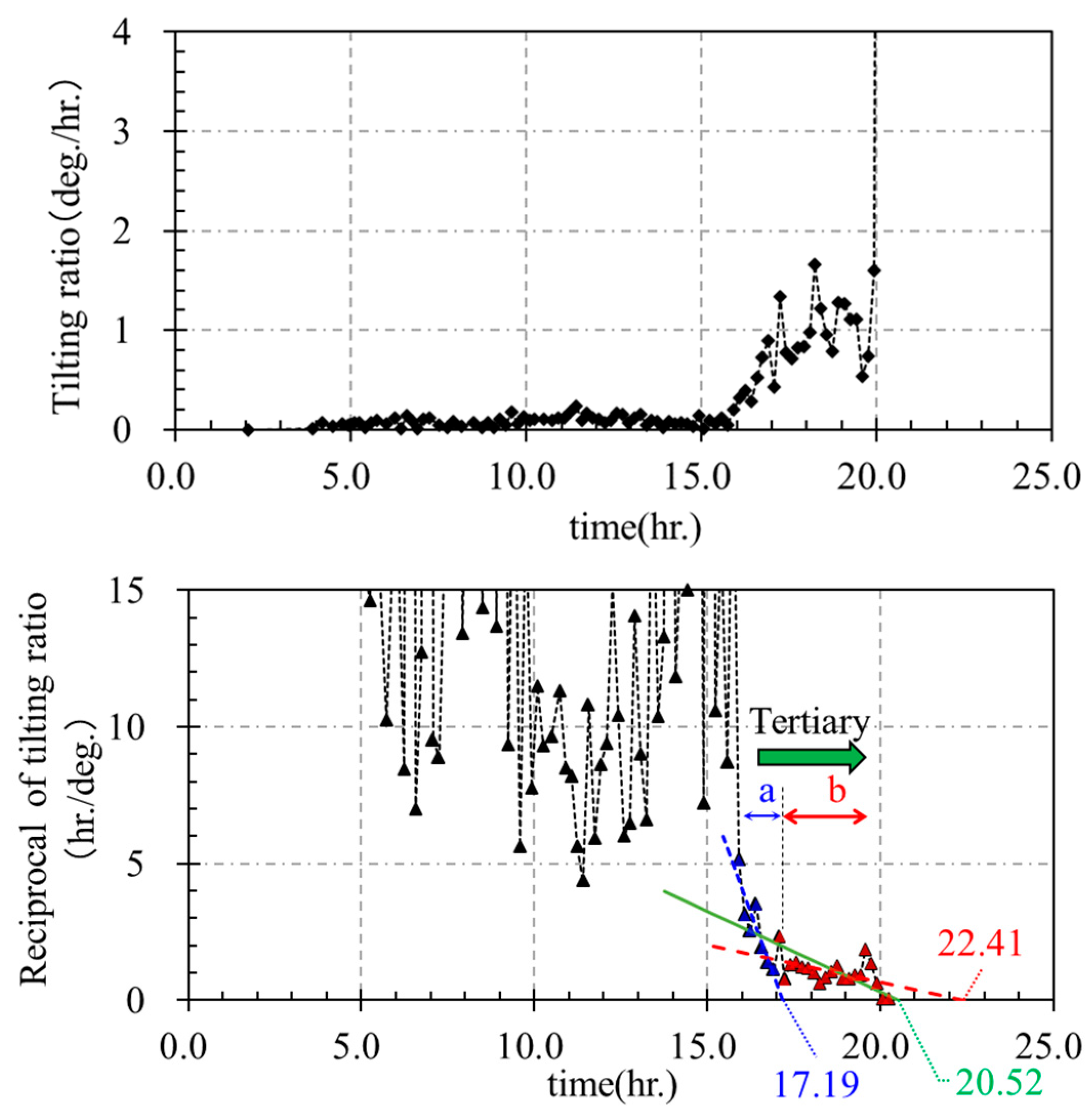
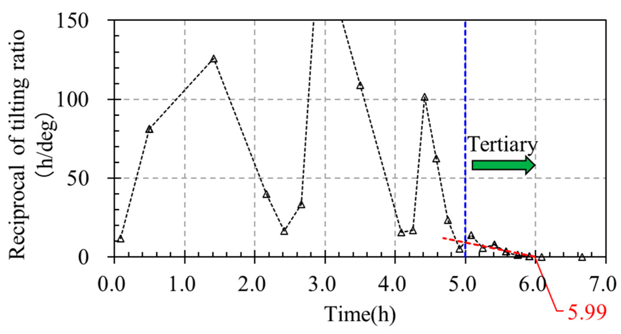
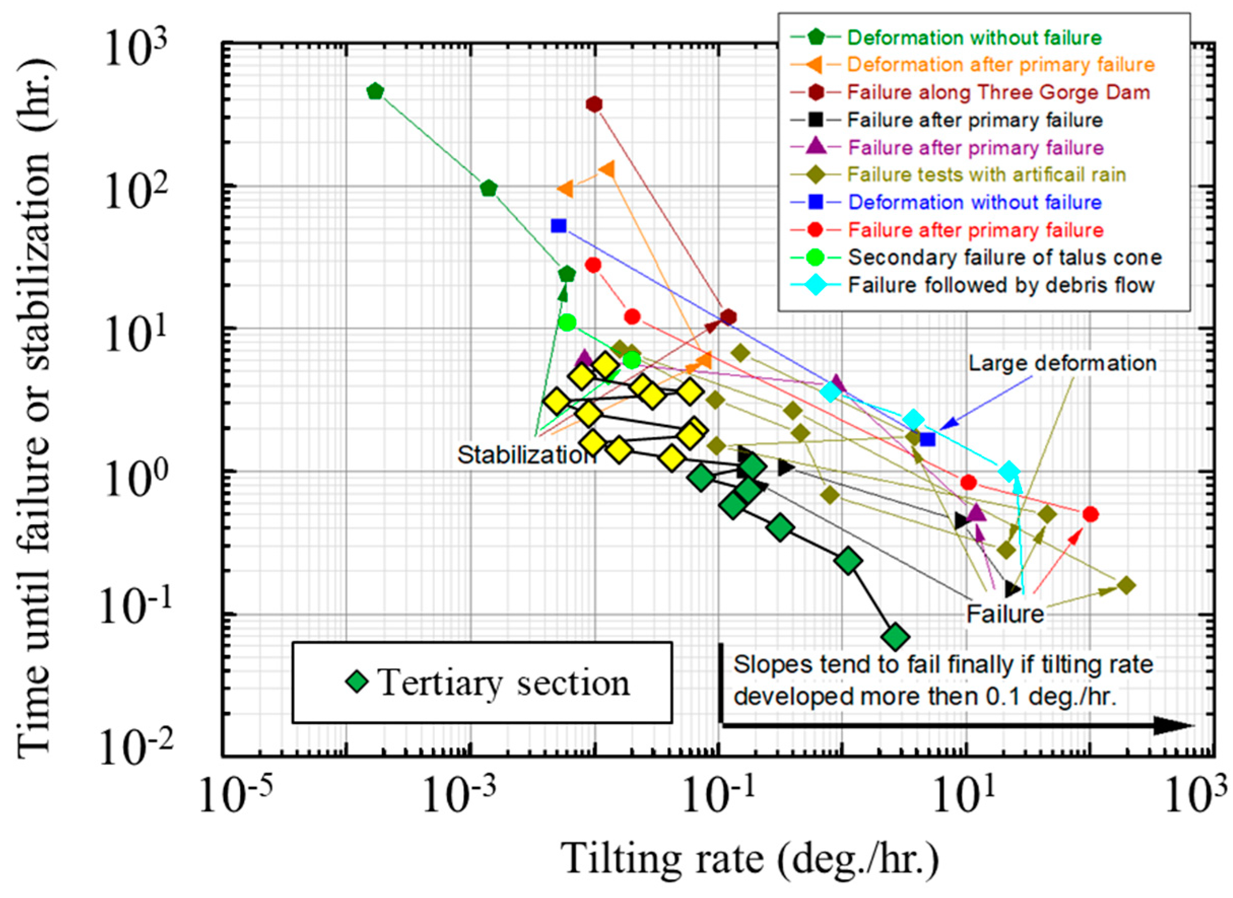
In the tertiary state of creep, the relationship between the velocity of the tilt angle and the time until failure can be expressed as an inverse proportional relationship. This means that as the time until failure decreases, the velocity increases proportionally.

(2)

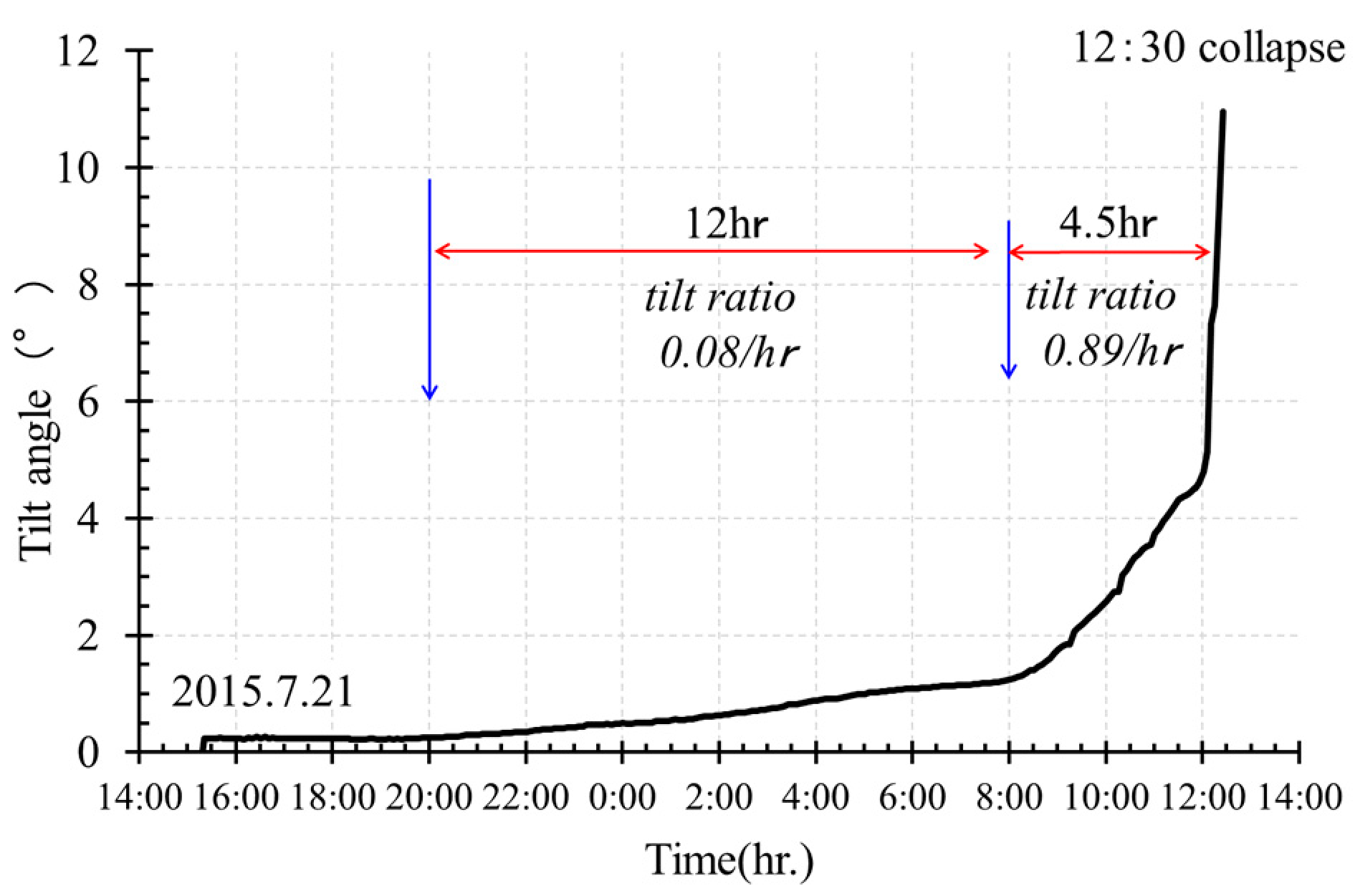
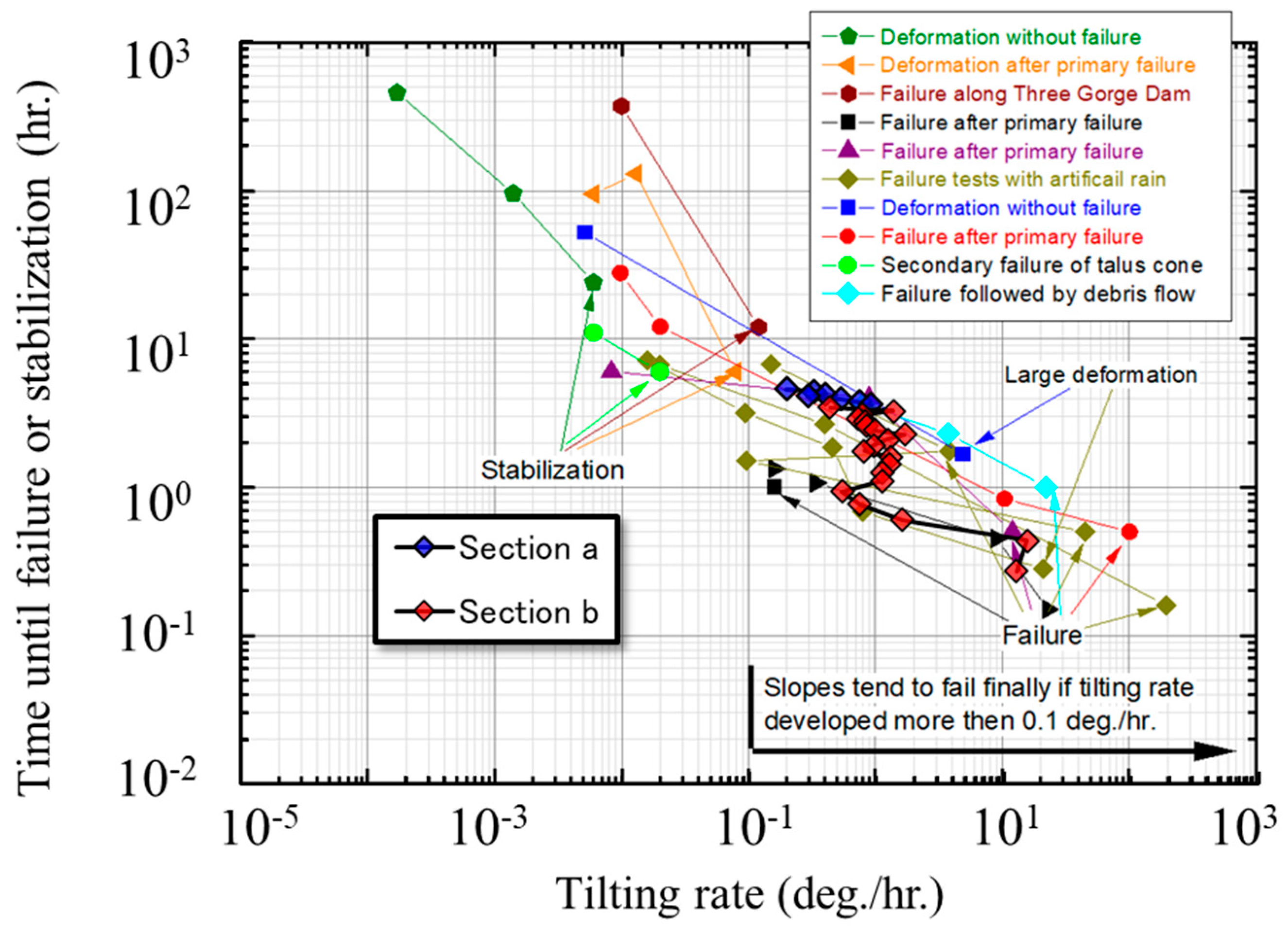
When the velocity of the tilt angle reaches the tertiary creep stage, ranging from 0.01°/h to 0.1°/h, an alert message can be sent. If it exceeds 0.1°/h, a warning message can be sent. This two-stage warning threshold is a reasonable value and can serve as a guideline for an early warning threshold.

The characteristics of landslides and slope failure can vary significantly due to a variety of factors, including geological conditions, water saturation levels, gravitational forces, frictional forces, and the type of movement involved. Therefore, further investigations are necessary to determine whether this method can be effectively utilized to predict the failure time for any landslides and slopes.

References

1. Mirus, B.B.; Jones, E.S.; Baum, R.L.; Godt, J.W.; Slaughter, S.; Crawford, M.M.; Lancaster, J.; Stanley, T.; Kirschbaum, D.B.; Burns, W.J.; et al. Landslides across the USA: Occurrence, Susceptibility, and Data Limitations. Landslides 2020, 17, 2271–2285. [Google Scholar] [CrossRef]
2. Pozzobon, M.; da Silveira, C.T.; Curcio, G.R. Landslides Susceptibility Analysis in Blumenau, Southern Brazil: A Probabilistic Approach. Int. J. Eros. Control Eng. 2019, 11, 63–72. [Google Scholar] [CrossRef]
3. Haque, U.; Blum, P.; da Silva, P.F.; Andersen, P.; Pilz, J.; Chalov, S.R.; Malet, J.P.; Auflič, M.J.; Andres, N.; Poyiadji, E.; et al. Fatal Landslides in Europe. Landslides 2016, 13, 1545–1554. [Google Scholar] [CrossRef]
4. Peruccacci, S.; Brunetti, M.T.; Gariano, S.L.; Melillo, M.; Rossi, M.; Guzzetti, F. Rainfall Thresholds for Possible Landslide Occurrence in Italy. Geomorphology 2017, 290, 39–57. [Google Scholar] [CrossRef]
5. Runqiu, H. Some Catastrophic Landslides since the Twentieth Century in the Southwest of China. Landslides 2009, 6, 69–81. [Google Scholar] [CrossRef]
6. Yamagishi, H.; Shimura, K.; Kurata, T. Landslides along the Coast from Ainuma to Toyohama, Southwestern Hokkaido, Japan. Landslides 1995, 31, 23–29. [Google Scholar] [CrossRef] [PubMed]
7. Onodera, T.; Yoshinaka, R.; Kazama, H. Slope Failures Caused by Heavy Rainfall in Japan. J. Jpn. Soc. Eng. Geol. 1974, 15, 191–200. [Google Scholar] [CrossRef]
8. Campbell, R.H. Soil Slips, Debris Flows, and Rainstorms in the Santa Monica Mountains and Vicinity, Southern California; US Government Printing Office: Washington, DC, USA, 1975; 51p. [Google Scholar]
9. Caine, N. The Rainfall Intensity: Duration Control of Shallow Landslides and Debris Flows. Geogr. Ann. Ser. A, Phys. Geogr. 1980, 62, 23–27. [Google Scholar]
10. Baum, R.L.; Godt, J.W. Early Warning of Rainfall-Induced Shallow Landslides and Debris Flows in the USA. Landslides 2010, 7, 259–272. [Google Scholar] [CrossRef]
11. Segalini, A.; Valletta, A.; Carri, A. Landslide Time-of-Failure Forecast and Alert Threshold Assessment: A Generalized Criterion. Eng. Geol. 2018, 245, 72–80. [Google Scholar] [CrossRef]
12. Saito, M. Failure of Soil Due to Creep. In Proceedings of the 5th International Conference SMFE, Paris, France, 17–22 July 1961; Volume 1, pp. 315–318. [Google Scholar]
13. Saito, M. Forecasting the Time of Occurrence of a Slope Failure. In Proceedings of the 6th International Conference on Soil Mechanics and Foundation Engineering, Montreal, Canada, 8–15 September 1965; pp. 537–541. [Google Scholar]
14. Saito, M. Forecasting Time of Slope Failure by Tertiary Creep. In Proceedings of the 7th International Conference on Soil Mechanics and Foundation Engineering, Mexico City, Mexico, 25–29 August 1969; pp. 677–683. [Google Scholar]
15. Fukuzono, T. A Method to Predict the Time of Slope Failure Caused by Rainfall Using the Inverse Number of Velocity of Surface Displacement. Landslides 1985, 22, 8–13_1. [Google Scholar] [CrossRef] [PubMed]
16. Uchimura, T.; Towhata, I.; Anh, T.T.L.; Fukuda, J.; Bautista, C.J.B.; Wang, L.; Seko, I.; Uchida, T.; Matsuoka, A.; Ito, Y.; et al. Simple Monitoring Method for Precaution of Landslides Watching Tilting and Water Contents on Slopes Surface. Landslides 2010, 7, 351–357. [Google Scholar] [CrossRef]
17. Crosetto, M.; Copons, R.; Cuevas-González, M.; Devanthéry, N.; Monserrat, O. Monitoring Soil Creep Landsliding in an Urban Area Using Persistent Scatterer Interferometry (El Papiol, Catalonia, Spain). Landslides 2018, 15, 1317–1329. [Google Scholar] [CrossRef]
18. Casagli, N.; Catani, F.; Del Ventisette, C.; Luzi, G. Monitoring, Prediction, and Early Warning Using Ground-Based Radar Interferometry. Landslides 2010, 7, 291–301. [Google Scholar] [CrossRef]
19. Massonnet, D.; Feigl, K.L. Radar Interferometry and Its Application to Changes in the Earth’s Surface. Rev. Geophys. 1998, 36, 441–500. [Google Scholar] [CrossRef]
20. Kromer, R.A.; Hutchinson, D.J.; Lato, M.J.; Gauthier, D.; Edwards, T. Identifying Rock Slope Failure Precursors Using LiDAR for Transportation Corridor Hazard Management. Eng. Geol. 2015, 195, 93–103. [Google Scholar] [CrossRef]
21. Malet, J.P.; Maquaire, O.; Calais, E. The Use of Global Positioning System Techniques for the Continuous Monitoring of Landslides: Application to the Super-Sauze Earthflow (Alpes-de-Haute-Provence, France). Geomorphology 2002, 43, 33–54. [Google Scholar] [CrossRef]
22. Monkman, F. An Empirical Relationship between Rupture Life and Minimum Creep Rate in Creep-Rupture Tests. Proc. ASTM 1956, 56, 593–620. [Google Scholar]
23. Tao, S.; Uchimura, T.; Fukuhara, M.; Tang, J.; Chen, Y.; Huang, D. Evaluation of Soil Moisture and Shear Deformation Based on Compression Wave Velocities in a Shallow Slope Surface Layer. Sensors 2019, 19, 3406. [Google Scholar] [CrossRef] [PubMed]
Figure 1. Creep model. (a) Metal creep model. Three creep stages are included in creep behavior before failure. Primary: strain rate decreases over time. Secondary: strain rate is constant. Tertiary: strain rate is rapidly increasing until failure. (b) Inverse velocity when α = 2 in Equation (2).
Geotechnics 04 00001 g001
Figure 2. A sample soil creep result of a laboratory experiment.
Geotechnics 04 00001 g002
Figure 3. Multi-layer shear model test apparatus. (a) presents a panoramic view of the experiment. The rainfall, at a rate of 60 mm/h, is coming down from the top and infiltrating into the specimen. Water can flow out from the bottom. (b) is a conceptual diagram of the multi-layer shear model. At every layer, a constant shear load is generated by the air cylinder, and the displacement is recorded by the meter sensor.
Geotechnics 04 00001 g003
Figure 4. Direct shear test apparatus. In (a), a movable layer and a fixed layer are included, and the vertical load and the horizontal load are applied at the movable layer. (b) shows the specimen inside the box at the initial stage.
Geotechnics 04 00001 g004
Figure 5. Grain size distribution curve.
Geotechnics 04 00001 g005
Figure 6. Temporal change in displacement (disp.) and inverse velocity (1/v).
Geotechnics 04 00001 g006aGeotechnics 04 00001 g006b
Figure 7. The relationship between time until failure and velocity.
Geotechnics 04 00001 g007aGeotechnics 04 00001 g007b
Figure 8. An image of covert displacement of the tilt angle. D is displacement, H is height, and θ is the tilt angle.
Geotechnics 04 00001 g008
Figure 9. Relationship between time to collapse and strain rate. (a) shows the analysis result of case 1, the tilt angle, tilt rate, and reciprocal tilt rate are represented in (a-1a-3). (b-1b-3) shows the analysis result of case 2.
Geotechnics 04 00001 g009
Figure 10. (a) Plot of the tilt rate (velocity) and the time until failure during tertiary creep in the lab experiment with the site measurements using the data for Case 1. (b) Plot of the tilt rate (velocity) and the time until failure during tertiary creep in the lab experiment with the site measurements using the data for Case 2.
Geotechnics 04 00001 g010
Figure 11. Observation results for slope angle and cumulative rainfall at Site A.
Geotechnics 04 00001 g011
Figure 12. Tilt rate and the reciprocal of the tilting ratio at Site A.
Geotechnics 04 00001 g012
Figure 13. Plot of the tilting rate and time until failure at Site A with previous site data.
Geotechnics 04 00001 g013
Figure 14. Observation results for the inclination angle of Site B (30 September 2018).
Geotechnics 04 00001 g014
Figure 15. Temporal variation in the tilting ratio at Site B.
Geotechnics 04 00001 g015
Figure 16. Temporal variation in the reciprocal of the tilting ratio at Site B.
Geotechnics 04 00001 g016
Figure 17. Plot of the tilting rate and time until failure at Site B with previous site data.
Geotechnics 04 00001 g017