1. Introduction
The dynamic interaction between soil and foundation is a complex phenomenon that poses significant challenges to geotechnical engineers. This challenge is especially pronounced when dealing with extreme loading conditions, material nonlinearity, changing boundary conditions, and large deformations common in dynamic pile–soil interaction under impact loading. Despite advancements in computational methodologies, accurately simulating this event remains daunting.
The updated Lagrangian finite element method (UL-FEM) has been a cornerstone in this computational landscape, yet it is not without its limitations. While UL-FEM has been instrumental in solving dynamic pile–soil interaction problems across various applications, it suffers from significant drawbacks. These include severe mesh distortions and element entanglements, often leading to non-physical and inaccurate results. Such issues are particularly prevalent in scenarios involving large deformations, such as “rigid” or “short” piles embedded in soil subjected to impact loading.
Four principal computational methodologies have gained prominence in the realm of simulating laterally impacted piles embedded in soil. These are the lumped parameter approach [
1,
2], the subgrade reaction method [
3,
4], the modified subgrade reaction approach [
5,
6], and the direct method [
5,
6,
7,
8,
9,
10,
11,
12,
13]. While the first three methodologies rely on nonlinear springs, dampers, and lumped soil mass to simulate the dynamic soil behavior, the direct method employs a continuum Lagrangian solid elements, adhering to specific constitutive laws. However, all these approaches bear intrinsic limitations. The abstraction of soil to nonlinear springs, dampers, and lumped mass fails to capture its complex particulate–continuum nature and often overlooks critical soil attributes, such as the dynamic stress–strain behavior of soil, the three-dimensional large plastic deformation of soil around the pile, the volumetric expansion behavior of the soil, strain rate and inertial effects on the behavior of soil, hydro-mechanical effects (fully saturated vs. unsaturated/partially saturated soil), and the dynamic shear interaction between the pile and the surrounding soil. This leaves these methods less reliable when complex impact loading conditions, multiphysics situations, complex pile geometries, and various terrain conditions (sloped vs. level terrain) are present.
Moreover, although the direct method excels in simulating soil responses under small deformations, it struggles with mesh distortions and element entanglements during larger deformations, particularly for simulations that involve “rigid” or “short” piles. Simulating pile–soil systems using a direct approach requires expertise in the computational modeling of geotechnical problems as well as the use and calibration of soil constitutive models.
In addition, previous research has disproportionately focused on inelastic pile deformations during pile–soil impacts, potentially obscuring the contribution of soil behavior to the overall system dynamics. This leaves several unresolved questions, especially about the soil mechanics that pile failure mechanisms might overshadow. Given these limitations and gaps in understanding, there is an urgent need to develop an improved and computationally efficient methodology. Specifically, computational frameworks engineered for large deformation problems are promising avenues for enhanced modeling of dynamic pile–soil interactions under impact scenarios, thus constituting an important frontier for deepening the understanding of the governing physics of pile–soil systems under extreme loading conditions.
In recent times, mesh-free particle techniques, such as smoothed particle hydrodynamics (SPH) [
14,
15] and the material point method (MPM) [
16,
17], have been recognized for their utility in modeling soil–structure interactions that encompass large soil deformations. However, the significant computational demands of these methods pose challenges for simulating large-scale pile–soil systems, especially under vehicular impacts. On the other hand, the discrete element method (DEM) [
18,
19,
20,
21,
22] emerges as an alternative, though its granular-scale methodology requires considerable computational resources. Moreover, this granularity often necessitates introducing scaling factors to efficiently model large soil volumes using fewer particles [
19,
20]. Notably, little of the prevalent MPM and DEM codes, either open-source or proprietary, is tailored for dynamic soil-structure scenarios associated with vehicular collisions.
Addressing this gap, this study presents an enhanced and computationally efficient approach—termed the erosion method—to model dynamic pile–soil interactions under impact loading. This method augments UL-FEM with an erosion algorithm to address the large deformations in granular soils around embedded piles during lateral vehicular impact events. To ensure the robustness and reliability of the erosion method, this study developed full-scale, mechanics-based computational models and validated them against field-scale physical impact tests.
This research aims to formulate a computationally efficient, large-deformation soil modeling methodology for use in nonlinear finite element analysis platforms, such as LS-DYNA [
23,
24]. This improved simulation method is pivotal for accurate simulations of soil-embedded barrier and containment systems, including W-beam and Thrie-beam guardrail systems and approach guardrail transitions (AGTs), during vehicular impacts. The main function of these barrier systems is to safely contain and redirect errant vehicles. The fulfillment of these needs largely depends on the dynamic soil–pile interaction during impact events, which affects the energy dissipation capability of soil-embedded vehicle barrier systems. This study also examined the influence of soil mesh density and pattern on the results of simulated pile–soil systems under lateral impacts. Initial analyses targeted the identification of mesh densities capable of capturing the soil’s large deformation and plastic flow dynamics during pile impacts. Subsequent investigations pivoted toward examining the effects of soil domain sizes and boundary conditions on the dynamic response of laterally impacted pile–soil systems. The intent was to investigate model response by varying domain sizes and boundary conditions and to develop guidelines for optimizing these parameters for enhanced accuracy and efficiency in pile–soil impact simulations.
2. Element Erosion Technique
The UL-FEM method employs fixed-mass elements wherein the mesh attached to the material also deforms when subjected to deformations. This results in severe mesh distortions for dynamic, large-deformation problems, such as vehicle impacts into pile–soil systems. Consequently, this problem introduces numerical instabilities, slows the calculations, and sometimes terminates the computation. In order to overcome these difficulties, the UL-FEM hydrocodes use an element erosion technique that deletes severely distorted elements to enable the computation to continue. Element erosion thresholds are set to avoid deleting the soil elements until they are severely damaged and their strength and mass are no longer likely to affect the physics of the problem.
Although the element erosion algorithm does not simulate the real physics of the pile–soil impact problem, it is a convenient numerical technique to avoid numerical problems associated with large soil deformations due to extreme loading conditions. Severe mesh distortion produces three major problems for geotechnical engineering applications that involve large and rapid deformation of soils. Firstly, the soil elements can invert, which results in negative Jacobian or negative volume, causing most hydrocodes to terminate the computation. Secondly, severe distortion produces errors in the evaluation of the soil constitutive equation, specifically when the soil element undergoes rapid deformation. Thirdly, it reduces the time step, which results in impractical or extremely long CPU time, as the time step is computed from the smallest element dimension.
Different element erosion criteria have often been used to model and analyze materials and structures under dynamic impact loading. These criteria are classified based on the variable that deletes severely distorted elements from the computation, such as strain-based [
25,
26,
27,
28,
29,
30], stress-based [
31,
32], and damage-based criteria [
33,
34]. Defining proper erosion characteristics is important in simulating dynamic pile–soil interaction under impact loading. If the soil elements are deleted too soon, the soil may offer less resistance to the pile impact, making the pile move farther into the soil with minimal resistance provided by the soil. On the other hand, if the failure strain or stress is set too high, soil elements may be severely distorted, reducing the computation time step and, in some cases, leading to the termination of the simulation. Therefore, choosing element deletion values is typically a trade-off between preventing deletion for as long as possible and not sacrificing accuracy or computational cost due to the element distortion.
Among the various element erosion criteria, the damage-based criterion is associated with the stiffness degradation of the material, making it physically sound and adequate for modeling the large deformation of geomaterials [
35]. However, a continuum damage model should be incorporated into the soil constitutive model to implement the damage-based erosion criterion for deleting severely distorted soil elements. Since the soil material model used in this study includes a continuum damage model, utilizing a damage-based element erosion criterion is relatively straightforward.
3. Constitutive Models
The choice of proper constitutive models that can account for the critical behavior of soil and pile and calibrate input parameters under dynamic impact environments is vital to accurately model and evaluate the dynamics of vehicle impacts into piles embedded in soil. This section details the prevailing constitutive model used for modeling the impact behavior of the soil and steel (pile) material for simulating and modeling dynamic pile–soil interaction problems using the erosion method.
3.1. Granular (MASH Strong) Soil
In accordance with the stringent protocols governing soil-embedded barriers and containment system crash tests, steel piles are frequently embedded in granular soils, hereafter referred to as granular (MASH strong) soil. As shown in
Figure 1, the granular (MASH strong) soil exhibits heterogeneity in grain sizes, characterized by a spectrum of angular to subangular particles, spanning dimensions from 19.05 mm down to silt-sized particles. Through the lens of the Unified Soil Classification System (USCS), granular (MASH strong) soil can be systematically classified under the well-graded gravel (GW) category.
A rheological soil model (FHWA soil model) that is available within the LS-DYNA simulation platform is adopted to simulate granular (MASH) strong soil. An in-depth discussion on the FHWA granular soil model for modeling dynamic impact soil–pile interaction is provided in [
36]. The details regarding this soil constitutive model are not discussed herein; however, a brief description of the FHWA granular soil model is discussed below.
The FHWA soil model is specifically developed to model dense and rapid granular flows of compacted road-base material, also known as NCHRP Report 350 strong soil [
37], utilized in full-scale crash testing of soil-embedded vehicle barrier systems. It should be noted that the NCHRP Report 350 strong soil is most similar to granular (MASH strong) soil. This constitutive model has been recognized as the most appropriate (granular) soil model within LS-DYNA for simulating the elastoplastic behavior of soil, including the influence of soil confinement, strain rate, strain softening or damage, pore water pressure, and moisture [
38,
39,
40,
41].
The FHWA soil model is developed within the elasto-viscoplastic constitutive framework. The elastic behavior is based on Hooke’s law (i.e., isotropic linear elasticity). The condition of plastic yielding is based on a modified Mohr–Coulomb yield function that relates the deviatoric stresses with the hydrostatic pressure exerted on the granular soil. The elastic condition allows the granular soil to have a stagnant configuration. In contrast, the plastic condition enables the granular soil to yield when the stress state reaches the shear strength of the granular soil. The FHWA soil model included a viscoplastic regularization of the continuum damage model via a Duvaut–Lions type of viscoplastic formulation to model the rapid, dense flow of compacted granular (MASH strong) soil during pile impacts.
The regularized softening or damage model enables the FHWA granular soil model to account for the large soil deformation as well as to capture the transition to fluid-like soil flow, including liquefaction-like behavior that is typically observed during crash testing of piles embedded in granular soil.
Table 1 presents the calibrated granular (MASH strong) soil model parameters utilized in this study. The methodology for selecting and determining model input parameters relevant to granular (MASH strong) soil is presented in reference [
36]. Furthermore, reference [
36] offers a comprehensive analysis of the range of input parameter values for the FHWA soil model for simulating dynamic impact soil–structure interaction problems.
3.2. Steel Pile
The piecewise-linear plasticity model [
23,
24], was used to model the steel piles. In the piecewise-linear plasticity model, the deviator stress is determined to satisfy the yield function as follows:
in which
sij is the deviator stress tensor, and
where
β is a strain-rate factor and accounts for strain-rate effects;
is the initial yield stress; and
is the hardening function and can be specified in tabular form or linear hardening of the form
with plastic hardening modulus
Ep.
In this elastoplastic model, the deviator stresses are updated elastically, and the yield function is checked. The deviator stresses are accepted if the yield function is satisfied. Otherwise, the plastic strain increment is calculated as follows:
in which
Ep is the current hardening modulus, and
G is the shear modulus. The trial deviator stress state,
, is scaled back as follows:
The piecewise-linear plasticity model accounts for strain-rate effects using the Cowper–Symonds model. The Cowper–Symonds model scales the yield stress using a factor
β, which is calculated as
in which
is the effective plastic strain rate, and
c and
p are Cowper–Symonds strain-rate parameters.
The extraction of Cowper–Symonds strain-rate parameters from tensile tests is not feasible. Nevertheless, Symonds [
42] reported that, for mild steel, the parameters with values of 40.4 for parameter
c and 5 for parameter
p demonstrate a reasonable correlation with experimental observations. Consequently, these specified values for
c and
p were adopted as the input parameters within the piecewise-linear plasticity model for the simulation of steel piles.
The tensile tests conducted on “dog bone” samples extracted from W152 × 12.6 piles at MwRSF-UNL and reported in the work of Schmidt et al. [
43] were used to obtain the material properties of the American Society for Testing Materials (ASTM) A36 steel pile.
Table 2 shows the material input parameters for the ASTM A36 steel pile. Similarly, the material properties for the ASTM A992 steel pile were obtained from tensile tests conducted on samples extracted from a W152 × 23.6 ASTM A992 steel pile at MwRSF-UNL and reported in the work of Schrum et al. [
44]. The material input parameters for the ASTM A992 steel pile are presented in
Table 3.
3.3. Erosion Criteria
In this work, the removal of Lagrangian soil elements—conceptualized as element erosion—is triggered when the damage and principal failure strain cross a threshold value. Within the FHWA soil model, DAMLEV signifies the damage level, ranging between 0 and 1.0, and determines element erosion in soil material [
23]. Concurrently, ‘EPSMAX’ demarcates the maximum principal failure strain causing the removal of a solid element. Therefore, both DAMLEV and EPSMAX thresholds must be exceeded to invoke the deletion of a soil element. DAMLEV and EPSMAX were equalized with the maximum damage parameter (
Dmax) to incorporate element erosion into the soil model. As depicted in Equation (6), the maximum damage within the soil element is associated with the peak (
) and residual (
) friction angles of the soil. These values for element erosion were utilized as adaptivity thresholds in simulating various post-soil systems subjected to lateral impact loading.
The FHWA soil model incorporates a mechanism to simulate damage, factoring in the void formation parameter,
Gf, and volumetric strain at the initial damage threshold,
. The void formation parameter, representing the area under the softening region in the pressure–volumetric strain curve, is quantitatively described as
where
V is the volume of the element,
P is the peak pressure,
is the volumetric strain, and
a is the element-dependent strain at full damage.
The transition from an undamaged (
) to a damaged stress (
,) state is captured by the following relationship: damaged stress,
, is found from undamaged stress, as follows:
with
D representing the isotropic damage parameter that modulated the effective internal stress, transitioning from 0 (undamaged) to 1 (failure).
The evolution of isotropic damage parameter,
D, is given by
in which
α and
are strain-softening input parameters, corresponding to the strain at full damage and the volumetric strain at the initial damage threshold, respectively.
The criterion for strain energy-based damage,
, is formulated as
where
K is the bulk modulus, and
is the plastic volumetric strain.
Lastly, the strain at full damage,
α, is extracted from the finite element volume by
4. Model Development and Simulation Details
Numerical models were developed to assess the capability of the erosion method in simulating laterally impacted pile–soil systems under various scenarios. First, the impact response of a flexible pile installed in soil was evaluated, mirroring a physical impact test performed on a W152 × 12.6 steel pile of 1830 mm length, embedded 1016 mm into MASH strong soil. Next, the study encompassed a pile–soil system primarily governed by soil failure rather than pile yielding or plastic deformation. To this end, a numerical model was established to reproduce a physical impact test conducted on a W152 × 23.6 stiff steel pile of 1830 mm length, embedded (1016 mm) in MASH strong soil. To facilitate appropriate comparisons with physical impact test data, all simulations were conducted for a 100 ms impact event or a pile displacement threshold of 750 mm. The impetus for selecting a displacement threshold of 750 mm was twofold. Firstly, it aligns with the objective of benchmarking the simulation results against physical impact test data. Such correlation ensures that our computational approach retains fidelity compared to observed phenomena. Secondly, it serves to rigorously assess the efficacy of our proposed methodology in replicating large soil deformations, which are critical in understanding the complex interactions during pile–soil impact events. All computational tasks were executed using MPP LS-DYNA hydrocode, version R10.1.0, on the University of Nebraska’s Crane supercomputer cluster, equipped with Intel Xeon E5-2670 2.6 GHz processors and allocated 32 cores per simulation.
The computational model geometry, set-up, and initial conditions are shown in
Figure 2. The pile was composed of 3660 four-noded, fully integrated, square shell elements along the two flanges and 2562 four-noded, fully integrated, square shell elements along the web of the W152 × 12.6 pile. The shell elements along the web and flanges were 10 mm long across the pile height of 1830 mm.
The soil domain dimensions selected were 4 d × 4 d in plan and 2.5 d in depth, where d represents the pile embedment depth. This decision was made to keep the boundary effects outside the large deformation zones. The domain was formed by a 4000 mm × 4000 mm area extending to a depth of 2500 mm, divided into 3,057,070 hexahedral elements with single-point quadrature. Each element’s depth was 20 mm within the embedment region and 40 mm outside this zone. Variable mesh sizes were used on the X–Y plane, scaling down to a minimum of 5 mm × 10 mm around the pile to capture the large soil deformations during impact with enhanced fidelity. This minimum mesh zone had an area of 914 mm × 914 mm, based on high-speed video analysis from various physical impact tests conducted at the MwRSF-UNL.
For regions that were expected to undergo minimal plastic deformation, located at the farthest extent from the point of impact (far-field soil domain), the maximum mesh dimension was set to 40 mm × 40 mm. The soil domain size and mesh density were selected based on the dimensions of soil models used in the works of Sassi [
5], Sassi and Ghrib [
6], Wu and Thompson [
8], and Whitworth et al. [
13].
The acceleration data were taken from a nodal point at the center of gravity of the simulated bogie vehicle and processed similarly with the impact test data. The extraction of forces was facilitated using Newton’s second law, and the displacements were determined by double-integrating the acceleration data, given the initial velocity of the bogie vehicle before impact. The trajectories of these forces and displacements were aligned in the direction of impact. The energy dissipation characteristics of the pile–soil system were quantified by integrating the area under the force–displacement response curves.
It should be noted that a high-precision retroreflective optic speed trap was employed to measure the bogie vehicle’s initial speed in the physical impact tests. This apparatus comprised four equidistantly positioned retroreflective targets, each separated by roughly 450 mm, affixed to the vehicle’s side. Upon reflection of the emitted light by these targets, the corresponding emitter/receiver unit emitted signals received by a data acquisition system operating at a sampling rate of 10,000 Hz. Concurrently, an external LED box was triggered to emit flashes. The vehicle’s velocity was deduced from the temporal measurement between these signals and the known spatial interval of the targets. To ensure robustness in the speed measurements, LED illumination and high-speed digital video analysis were established as supplementary verification methods, particularly in instances where electronic readings were unattainable. This two-tiered approach enhances the integrity of the velocity data, strengthening the foundational parameters of the physical impact tests.
In the LS-DYNA numerical simulations, the interaction between the neoprene impact head of the bogie vehicle and the steel pile was carefully analyzed using the automatic node-to-surface contact algorithm. To accurately represent the frictional behavior between these two materials, static and dynamic friction coefficients were uniformly set at 0.1, based on empirical findings reported by Deladi [
45]. This approach aligns with best practices in dynamic impact simulations, which suggest equilibrating static and dynamic friction coefficients. This measure helps prevent numerical instabilities and suppress the excitation of unrealistically high-frequency contact phenomena, as discussed in the literature [
23,
24].
A penalty-based, two-way, eroding surface-to-surface contact was implemented to model the interaction between the pile and soil. Eroding surface-to-surface contact enables compression and tangential loads to be transferred from the master (pile) and slave segments (soil) and vice versa. Contact surfaces are also updated as soil elements are eroded. The force that prevents penetration between segments depends on the stiffness of linear springs. The contact stiffness is independent of the material properties of the pile and soil and is calculated by dividing the nodal masses with the square of the time step [
23,
24]. The static coefficient of friction was based on the peak friction angle of the soil, denoted by
, and was set as
. This approach follows the guidelines provided by Yoshimi and Kishida [
46] and Uesugi and Kishida [
47]. To ensure computational stability and to prevent non-physical high-frequency contact effects, the static and dynamic coefficients of friction were equated, as per standard modeling practices.
The simulations utilized the boundary non-reflecting (BNR) boundary conditions to emulate an infinite continuum and prevent artificial reflections of stress waves. The loading sequence was designed to closely mimic physical reality. The simulations began with an explicit dynamic relaxation mechanism that incrementally applied gravitational forces to the pile–soil system. This phase allowed the system to attain an equilibrium state reflective of an appropriate initial stress condition. After system stabilization, a transient impact load was applied by imparting an initial velocity to the computational bogie vehicle, mirroring the real-life impact scenario observed during the physical impact tests.
5. Simulating the Impact Response of Flexible Pile in Soil
5.1. Comparison between Simulation and Physical Impact Tests
A computer simulation of a bogie impacting an 1830-mm long, W152 × 12.6 steel pile embedded in granular (MASH strong) soil at a speed of 8.94 m/s was completed to assess the accuracy of the erosion method for simulating the dynamic pile–soil interaction problems that are primarily governed by pile failure or plastic bending instead of soil failure. The pile was embedded 1016 mm into the soil, and the volume was modeled using the erosion method. Results were compared against large-scale dynamic impact tests of a bogie vehicle impacting piles embedded in granular (MASH strong) soil. Quantitative comparisons focused on force vs. displacement response, energy vs. displacement response, and average impact forces with test nos. MH-1 and MH-4 from Schmidt et al. [
43] being selected for comparisons. The bogie vehicle impacted the pile at a speed of 9.30 m/s for test no. MH-1 and at 8.90 m/s for test no. MH-4.
Comparisons of the simulation results with the dynamic impact testing results are shown in
Figure 3 and provided in
Table 4. The most important results for comparison purposes were an average force at 125 mm, 250 mm, 375 mm, and 500 mm of pile displacement (measured at the impact point). These forces are essential for designing and analyzing soil-embedded barrier systems subjected to vehicular impacts. These forces were obtained by dividing the energy by the respective displacements [
48].
The average forces at pile displacements of 125 mm, 250 mm, 375 mm, and 500 mm from the numerical simulation were within 6.2%, 16.2%, 7.2%, and 0.2%, respectively, compared to the average (average forces) of the impact tests, as presented in
Table 4. The total energy obtained from the simulation was within 6.9% compared to the average total energy of the dynamic impact tests. Variances within 20% of the empirical data are generally considered reasonable for crash simulations [
49]. Thus, these results were deemed reasonable and satisfactory for the complex dynamic impact pile–soil interaction problem.
Post-impact photographs from the simulation were compared with those observed in test no. MH-1, as shown in
Figure 4. The simulation replicated the global behavioral patterns of the system, as evidenced by the correspondence between the predicted and observed deformed configurations, as well as the locations of local buckling and regions manifesting plastic deformation. A comparative examination of the final deformation states of the pile revealed a similarity in the permanent set and localized plastic deformation patterns. Notably, the computational model demonstrated the complete yielding of the pile, attributable to lateral-torsional buckling, occurring 265 mm beneath the ground surface. This finding is in close agreement with empirical observations from test nos. MH-1 and MH-4, wherein the W152 × 12.6 steel pile exhibited yielding at a depth approximately 254 mm below the ground surface [
43], highlighting the model’s accuracy in capturing the response of the pile under lateral impact loading.
5.2. Discussion of Results
The simulation predicted higher resistive forces at pile displacements ranging from 80 mm to 260 mm, as is evident from
Figure 3. This anomaly could be associated with the yielding of the pile due to lateral-torsional buckling. It is recognized that the current steel material model and its input parameters may not have sufficiently captured the complex phenomena of lateral-torsional buckling. Furthermore, there could be a potential influence of geometric imperfections on the simulation results, particularly beyond the threshold of plastic deformation. Such geometric imperfections could affect the accuracy of simulation results following the onset of plastic flow.
In light of these insights, we suggest that future research endeavors should be directed toward an exhaustive examination of the implications of steel constitutive models and their parameters, as well as the role of geometric imperfections in influencing the dynamic response of flexible piles embedded in granular soils. Despite these factors, it is crucial to emphasize that the simulation results, in terms of average resistive forces, align within an acceptable margin of error in relation to the physical impact test data.
Figure 5 and
Figure 6 reveal that the dynamic bending moment induced by lateral impacts surpasses the yield moment for the pile section. It can be inferred that for a W152 × 12.6 pile, with an embedment depth of 1016 mm in MASH strong soil, its lateral impact response was predominantly dictated by the properties of the pile itself. This behavioral pattern aligns with what is conventionally recognized in geotechnical engineering as a ‘flexible’ or ‘long’ pile failure mechanism. The graphical representations in
Figure 5 and
Figure 6 illustrate the formation of a plastic hinge, signifying that the pile–soil system’s impact resistance hinged upon the dynamic yield moment of the pile. This critical yield moment was attained prior to the full activation of the dynamic soil resistance. Moreover, it was observed that the soil manifests its complete dynamic resistance simultaneous with, but not exceeding, the steel pile’s yield threshold, as depicted in
Figure 6.
The contours of von Mises stress variations in the soil at different times presented in
Figure 6 show that plastic deformation of the soil primarily occurs in the near-field soil domain where the pile deformed plastically. The results from the stress analysis indicate that the impact resistance to yielding provided by the soil below the yield point is infinite, and the rotation of the pile cannot happen. The lower part of the embedded pile region remained mostly vertical, while the upper part deformed to a shape shown in
Figure 6.
6. Simulating Impact Response of Rigid Pile in Soil
6.1. Comparison between Simulation and Physical Impact Tests
A numerical simulation of a bogie impacting an 1830-mm long, W152 × 23.6 steel pile embedded in granular (MASH strong) soil at a speed of 9.84 m/s was completed to assess the accuracy of the proposed soil modeling method (tool) to simulate pile–soil systems primarily governed by soil failure, rather than pile yielding or plastic deformation. The pile was embedded 1016 mm into the soil, and the soil volume was modeled using the erosion method. Simulation results were compared to large-scale dynamic impact tests of a bogie vehicle impacting a W152 × 23.6 steel pile embedded in MASH strong soil. Quantitative comparisons focused on force vs. displacement response, energy vs. displacement response, and average impact forces with test nos. BL-8 and BL-20 being selected for comparisons. The bogie vehicle impacted the pile at a speed of 9.84 m/s for test no. BL-8 and at 9.21 m/s for test no. BL-20. The mass of the bogie vehicle, including accelerometers and the mountable head, was 783 kg and 842 kg, in test no. BL-8 and test no. BL-20, respectively.
Comparisons of simulation results with dynamic impact testing results are provided in
Table 5 and shown in
Figure 7. Again, the most important results for comparison purposes were the average forces at 125 mm, 250 mm, 375 mm, and 500 mm of pile displacement, and the total energy absorbed by the pile–soil system. The average forces at pile displacements of 125 mm, 250 mm, 375 mm, and 500 mm from the numerical simulation were within 18.1%, 11.8%, 0.3%, and 5.0%, respectively, compared to the (average) forces of the physical impact tests. The total energy obtained from the simulation was within 20% compared to the average total energy of the dynamic impact tests. As noted previously, results from simulated dynamic impact events within 20% of a test are typically considered reasonable [
49]. Thus, these results were deemed reasonable and satisfactory for the complex dynamic impact pile–soil interaction problem.
6.2. Discussion of Results
There is a slight overestimation of average resistive forces at a pile displacement of 125 mm, as presented in
Table 5. While there appears to be a minor deviation when compared to pile displacements at 250 mm, 375 mm, and 500 mm, pinpointing a definitive cause for this variance is challenging due to the intricacies inherent in the dynamic impact process. However, it is imperative to note, as illustrated in
Figure 7b, that the energy profiles generated by the computational model are consistent with the experimental data, both qualitatively and quantitatively. This suggests that, despite the slight overestimation at one displacement metric, the model effectively replicates the fundamental characteristics of the energy absorption and dissipation behaviors observed during the physical impact tests.
In contrast to the “long” or “flexible” pile, i.e., W152 × 12.6 with an embedment of 1016 mm, the behavior of the W152 × 23.6 pile with an embedment of 1016 mm is primarily governed by lateral soil failure instead of the yielding of the pile, as presented in the time-sequential photographs of the physical impact tests and simulated in
Figure 8. The lateral impact load caused the failure of the granular (MASH strong) soil along the entire pile length, as depicted in the effective (von Mises) stress contours in
Figure 9. Therefore, a 152 × 23.6 pile with an embedment of 1016 mm behaves essentially as a “short” or “rigid” pile, and the dynamic soil resistance governs its impact behavior, load capacity, and energy dissipation.
7. Effect of Soil Mesh Density on Response of Laterally Impacted Pile–Soil Systems
This study examined the effect of soil mesh density around the pile during lateral vehicular impacts. The objective of this investigation was to provide better insight into the influence of soil mesh density on the dynamic response of the pile–soil system. Further, it was desired to provide guidelines and recommendations on soil mesh densities (sizes) for pile–soil impact simulations using the erosion method.
7.1. Model Geometry and Discretization
In order to fulfill the above objective, two mesh densities were considered: (1) baseline mesh-size model (
Figure 10), which varied in the global X and Y directions based on distance from the pile, and (2) uniform mesh-size model (
Figure 11), which had a uniform soil mesh configuration around the pile. For the noted investigation, a 2134-mm long, ASTM A500 Grade B steel tube pile (i.e., a 152 mm × 203 mm with a wall thickness of 4.76 mm) embedded in granular (MASH strong) soil was considered. The focus was on the large-deformation soil zone (near-field soil domain) around the pile, which was 914 mm × 914 mm in the global
X–
Y plane. As noted previously, this large-deformation soil zone was determined based on observations from various physical impact tests conducted on pile–soil systems.
7.2. Results
Results from the simulation were compared with large-scale dynamic impact tests where a bogie vehicle impacted a steel tube pile set within granular (MASH strong) soil. The focal metric for comparison was the average impact force versus pile displacement, with data from test no. P3G-7, as documented by Meyer et al. [
50], which were chosen as the benchmark. The average force holds significance in the design and analysis of soil-embedded barriers and containment systems facing vehicular impacts [
48]. A comparison, encapsulating average forces and percentage differences between the simulated and physical test results, is shown in
Figure 12. This comparison is specifically rendered for average forces spanning pile displacements from 125 mm to 500 mm, as illustrated in
Figure 12b.
The simulation-derived average forces resonated well with those recorded during dynamic impact tests. For pile displacements at 125 mm, 250 mm, 375 mm, and 500 mm, the baseline mesh-size simulation deviated by 9.2%, 2.1%, 4.6%, and 6.2%, respectively, from the physical test data. Conversely, the uniform mesh-size simulation showcased deviations of 1.2%, 10.2%, 4.8%, and 1.2%, respectively, for the same displacements. Both simulation approaches—baseline and uniform meshes—yielded results within a 5% to 10% range of the physical impact test.
7.3. Guidelines and Recommendations
The findings presented in the previous section suggest that pile–soil impact models constructed with soil mesh sizes of 1 to 1 and 1 to 2 or (2 to 1) element aspect ratios within the large-deformation soil region as well as an element aspect ratio not more than 5 to 1 or (1 to 5) for the entire soil volume (domain) could replicate the essential responses of the dynamic impact pile–soil interaction problem. Pile–soil impact simulation models constructed with soil mesh sizes between 10 mm × 20 mm × 20 mm and 50 mm × 50 mm × 20 mm, as well as with soil mesh sizes between 10 mm × 10 mm × 10 mm and 50 mm × 50 mm × 10 mm show favorable agreement with physical impact test data in terms of pile–soil systems’ resistive forces and energy absorption. Thus, it is recommended that a constraint of no more than a 5 to 1 (or 1 to 5) soil element aspect ratio with mesh sizes between 10 mm × 10 mm × 10 mm and 50 mm × 50 mm × 10 mm be used for pile–soil impact simulations within the framework of the erosion method.
It is well known that significant mesh size differences between adjacent solid elements cause artificially induced excessive numerical errors in finite element analysis. Therefore, it is advisable to avoid abrupt soil element size differences among adjacent elements to avoid potential numerical errors in the pile–soil impact numerical simulation. As presented in this study, the soil models used a restriction of no more than 5 to 1 or (1 to 5) for the small deformation region and no more than 1 to 1 or 1 to 2 or (2 to 1) element aspect ratios for the large deformation zone satisfactorily predicted the impact behavior of the pile–soil system. Hence, a soil–element aspect ratio smaller than or equal to 5 to 1 or (1 to 5) was desirable for the pile–soil impact simulation.
Although the theoretical idealization of soil–element aspect ratios can be straightforward, it presents a complex challenge in practical application, particularly when dealing with dynamic impact analyses of large-scale pile–soil systems. Computational resources limit feasible model size and simulation duration, making it challenging to achieve simulation accuracy without compromising computational efficiency. This study systematically evaluated the effects of mesh configurations on the simulation results. It recommended a mesh density that aligns with the dual objectives of computational efficiency and simulation accuracy. The study also discussed how these configurations uphold the dynamic influences on pile–soil interaction even when the soil volume domain is altered.
The results presented, therefore, substantiate the selected element aspect ratio’s appropriateness and extend the discussion to include the dynamic interactions’ consistency across variable soil volume domains. This contribution is essential for advancing the understanding of mesh density effects on dynamic pile–soil interaction modeling and guiding future studies in this domain.
8. Effect of Soil Domain Size on Response of Laterally Impacted Pile–Soil Systems
When conducting any soil continuum-based computational analysis on dynamic pile–soil interaction problem, determining the size of the soil domain (volume) is essential. Theoretically, considering as large as possible of a soil volume would be ideal, as it produces dynamic responses free from boundary effects. Nonetheless, such a choice leads to enormous computational costs, and it is not feasible or practical for modeling full-scale, soil-based barrier and containment systems. Thus, it is important to justifiably define the size of soil volume for dynamic pile–soil interaction analysis that would ensure computational efficiency without the loss of accuracy of the dynamic response of the pile–soil system. In order to make the computational models more general and applicable for modeling various full-scale, soil-embedded barrier systems under vehicular impacts, the size of the soil domain was linked to the pile embedment depth (d).
8.1. Model Geometry and Discretization
Numerical simulations of a bogie vehicle impacting a 2134-mm long, ASTM A500 Grade B steel tube pile (i.e., a 152 mm × 203 mm with a 4.76 mm wall thickness and embedment depth (d) of 1219 mm) embedded in granular (MASH strong) soil at a speed of 10.95 m/s were completed to assess the effects of soil domain size on the results of dynamic impact pile–soil interaction. The soil volume was modeled using the erosion method following the previously discussed modeling methodologies and procedures. Six different soil volume sizes were considered, which were subjected to the previously mentioned impact conditions, and their response was monitored and analyzed. The soil volumes that were considered for this research effort were (1) 1.5d × 1.5d × 1.5d; (2) 2d × 2d × 1.5d; (3) 2d × 2d × 2d; (4) 3d × 3d × 2d; (5) 3d × 3d × 3d; and (6) 4d × 4d × 3d. An example of the details of the impact conditions, pile geometry, material properties, and the volume of soil domain utilized is provided in
Figure 13.
8.2. Results
The sensitivity of modeling results, including the force vs. displacement and energy vs. displacement responses of the pile–soil system to the various sizes of the soil domain, was examined to understand the influence of the soil domain size. The simulation results were compared with full-scale, physical impact testing data to quantify the change in pile–soil system response due to the size of soil volume.
Figure 14a shows a force vs. displacement and energy vs. displacement comparison between the impact test data from Meyer et al. [
50] and simulation with 1.5 d × 1.5 d × 1.5 d soil domain. The simulation showed a stiffer response for the initial 250 mm of pile displacements (at the impact height) compared to the physical impact test data. Additionally, there was an increase in the energy dissipation prediction for large pile displacements. The average force deviations between the simulation and the physical impact tests at pile displacements of 125 mm, 250 mm, 375 mm, and 500 mm were observed at 1.5%, 11.8%, 10.6%, and 9.2%, respectively. For the 2 d × 2 d × 1.5 d soil domain, as shown in
Figure 14b, the simulation overpredicted the resistive forces for pile displacements between 125 mm and 450 mm. The average force deviations at these displacements were 3.2%, 10.5%, 10.2%, and 9.4%, respectively.
Considering the 2 d × 2 d × 2 d soil domain, the simulations (
Figure 14c) revealed a stiffer response for displacements between 125 mm and 300 mm, accompanied by increased energy dissipation predictions for displacements beyond 250 mm. The force deviations at 125 mm, 250 mm, 375 mm, and 500 mm were 2.2%, 12.6%, 11.2%, and 7.3%, respectively. Within the 3 d × 3 d × 2 d soil domain,
Figure 15a compares the simulation and physical impact test. A slightly stiffer response is discernible between 125 mm and 400 mm displacements. The recorded average force deviations at 125 mm, 250 mm, 375 mm, and 500 mm pile displacement were 5.1%, 4.1%, 6.2%, and 4.7%, respectively.
In the context of the 3 d × 3 d × 3 d soil domain,
Figure 15b displays a notable alignment between the simulation and physical tests, particularly in force vs. displacement and energy vs. displacement. Discrepancies in forces at displacements of 125 mm (5 in.), 250 mm (10 in.), 375 mm (15 in.), and 500 mm (20 in.) were 6.8%, 3.1%, 4.2%, and 3.2%, respectively. Lastly, for the 4 d × 4 d × 3 d soil domain, as illustrated in
Figure 15c, the simulation mirrored the experimental data effectively. Discrepancies in average forces at displacements of 125 mm, 250 mm, 375 mm, and 500 mm were observed at 9.6%, 2.3%, 4.6%, and 3.2%, respectively.
In evaluating the dynamic response of the pile–soil system, differences were evident between the smallest and the largest soil domain sizes. With an increasing soil domain size, the pile–soil system response gradually converged towards the characteristics of larger soil domain sizes. Notably, the sensitivities in the system’s response were amplified for the smaller soil domain sizes, particularly for 1.5 d × 1.5 d × 1.5 d, 2 d × 2 d × 1.5 d, and 2 d × 2 d × 2 d configurations. In contrast, the responses manifested remarkable consistency across larger domain sizes, specifically in 3 d × 3 d × 2 d, 3 d × 3 d × 3 d, and 4 d × 4 d × 3 d. A significant change in both force vs. displacement and energy vs. displacement responses was observed upon the domain size increase from 1.5 d × 1.5 d × 1.5 d to 3 d × 3 d × 2 d.
Contrastingly, the difference was markedly subdued when the soil domain size increased from 3 d × 3 d × 2 d to 3 d × 3 d × 3 d. This observation highlights that past a specific soil domain size, the dynamic response of the pile–soil interaction experiences only negligible changes. Consequently, for engineering applications, there appears to be a defining soil domain size that accurately captures the pile–soil system’s dynamic behavior. This domain size can be categorically referred to as the “optimum soil domain size”. Delineating this optimum dimension can substantially reduce computational costs without sacrificing response accuracy. To ascertain this optimal size, it is imperative to undertake a computational time investigation across the discussed soil domain sizes. Pursuant to this, we executed a computational time analysis, laying down guidelines and recommendations for the optimal soil domain size pertinent to pile–soil system modeling. Subsequent sections discuss this computational time study.
9. Effect of Boundary Condition on Response of Laterally Impacted Pile–Soil Systems
In the context of pile–soil impact numerical analyses, the role of boundary conditions is paramount. For the baseline model, boundary non-reflecting (BNR) boundary conditions were applied to the exterior surfaces, encompassing four sides and bottom boundaries. Such a boundary condition mirrors real-world environments by negating the re-entry of artificially generated stress waves at soil model boundaries.
A contrasting approach adopted in numerous studies for soil–foundation system simulation is the single-point constraint (SPC) boundary condition (i.e., pinned or fixed boundary conditions). Herein, displacements and rotations are constrained [
51,
52,
53]. The comparative accuracy of BNR and SPC conditions in dynamic pile–soil interaction remains under-investigated in the existing literature. Past studies also offer limited guidance on optimal soil domain size and the most appropriate boundary conditions for dynamic impact pile–soil analyses. The present investigation probed the effects of BNR and SPC boundary conditions on the dynamic response of pile–soil systems across varied soil domain sizes. The subsequent section elucidates the derived insights.
9.1. Results
The dynamic response of pile–soil systems under varied boundary conditions was critically assessed across multiple soil domain sizes, determined by the pile’s embedment depth (d). Both BNR and SPC boundary conditions were considered. The soil domains evaluated included the following: 1.5 d × 1.5 d × 1.5 d, 2 d × 2 d × 1.5 d, 2 d × 2 d × 2 d, 3 d × 3 d × 2 d, 3 d × 3 d × 3 d, and 4 d × 4 d × 3 d.
The simulations’ average resistive force responses were compared against the physical impact test data.
Table 6 and
Table 7 present the difference in average force between the simulations (BNR and SPC conditions) and the physical impact tests from dataset P3G-7, measured at pile displacements of 125 mm, 250 mm, 375 mm, and 500 mm. Rather than gauging the computational efficiency of these models solely at a single CPU count, performances were assessed at 8, 16, 32, 64, and 128 CPU counts, as illustrated in
Figure 16 and
Figure 17. Additionally, the analysis duration, considering the number of solid soil elements and boundary conditions, was evaluated, detailed in
Figure 17. Based on these insights, subsequent sections provide consolidated guidelines and recommendations for pile–soil impact modeling and simulations using the erosion method.
9.2. Guidelines and Recommendations
Within pile–soil system dynamics, the fidelity of numerical simulations depends on the extent of the soil domain size and the boundary conditions adopted. An investigation into the system’s response for varied soil domain sizes revealed distinctive trends, highlighting the importance of these parameters for accurate modeling. For larger soil domain sizes, such as 3 d × 3 d × 2 d, 3 d × 3 d × 2 d, and 4 d × 4 d × 3 d, the response was less affected by boundary conditions. For instance, the 4 d × 4 d × 3 d domain exhibited a negligible influence from boundary conditions applied at both bottom and exterior boundaries. Therefore, responses at these sizes serve as an effective benchmark. On the contrary, the smaller soil domain sizes (1.5 d × 1.5 d × 1.5 d to 2 d × 2 d × 2 d) were significantly influenced by boundary conditions, especially the SPC type.
A discernable difference was observed in the system’s dynamic response between the smallest and largest domain sizes, regardless of the boundary conditions. As domain size increased, the system’s response became increasingly similar to larger domains for both BNR and SPC conditions. For instance, the shift from 1.5 d × 1.5 d × 1.5 d to 3 d × 3 d × 2 d elicited a pronounced change in force versus displacement and energy versus displacement response. However, this variation was subdued when progressing from 3 d × 3 d × 2 d to 4 d × 4 d × 3 d, implying that the dynamic response exhibits marginal alterations after a threshold. This observation emphasizes an “optimum soil domain size”—the ideal size that captures the system’s dynamic response without undue computational cost.
In light of computational efficiency, two regions of computation time trends exist, as discerned from
Figure 16 and
Figure 17. The initial region (8–32 CPUs) showcases a sharp rise in computation time with expanding soil domain size. Subsequently, an asymptotic trend emerges (32–128 CPUs) irrespective of boundary conditions. Importantly, BNR boundary conditions typically demanded 20% to 50% more computation time than the SPC.
A comparative analysis with the physical impact test data affirms that simulations with BNR boundary conditions across all evaluated soil domain sizes accurately model the dynamic response. Meanwhile, the domains of 3 d × 3 d × 2 d to 4 d × 4 d × 3 d with SPC boundary conditions offer a balance between accuracy and computational efficiency. Thus, these configurations are recommended for future numerical modeling endeavors of the pile–soil impact problem using the erosion method.
10. Summary, Conclusions, and Future Research
A computationally efficient, large-deformation soil modeling method, i.e., the UL-FEM enhanced by an erosion algorithm, referred to as the erosion method for the numerical simulation of the pile–soil impact problem, has been presented. The UL-FEM enhanced by an erosion algorithm has been combined for the first time with a continuum damage-based viscoplastic soil constitutive model, which realistically predicts the dynamic mechanical behavior of granular (MASH strong) soil. Comparisons between simulation and field-scale physical test results were discussed. The key findings from the study presented in this paper are highlighted below.
The proposed large-deformation soil modeling method for pile–soil impact analysis based on the element erosion algorithm within the UL-FEM framework agreed well the measured pile–soil impact response. The applicability of the soil modeling method has been successfully demonstrated for both “long” or “flexible” and “short” or “rigid” pile behavior under impact loading.
The simulation method presented in this study overcomes the inherent limitations of popular soil modeling techniques typically used for modeling piles embedded in soil under vehicular impacts, such as the lumped parameter method, subgrade reaction approach, modified subgrade reaction method, and direct method.
This study investigated the effect that soil domain sizes and boundary conditions had on the dynamic impact response of pile–soil systems using field-scale physical impact test data. This study should help engineers and researchers better understand the influence of soil domain sizes and boundary conditions on the dynamic response of piles embedded in granular soil when subjected to lateral vehicular impacts. Furthermore, guidelines and recommendations were provided on optimum soil domain size and boundary conditions.
Computational time studies were conducted to assess the efficiency of the various soil domain sizes and boundary conditions. This investigation demonstrated the effect that soil domain sizes and boundary conditions had on the performance of LS-DYNA pile–soil impact simulations.
The modeling method developed in this study can be used to enhance and advance the current pile–soil system modeling methods and be extended for future research, such as modeling full-scale, soil-embedded barrier and containment systems.
This research work will significantly contribute to the numerical modeling techniques currently used by engineers and researchers in the analysis and design of piles subjected to vehicular impact loading. The findings of this study will facilitate efficient and economically feasible pile design by reducing the required number of component crash tests of pile–soil systems.
The research presented herein has made substantive advances in soil modeling techniques for simulating dynamic impact interactions within pile–soil systems. The erosion method introduced in this paper has undergone rigorous validation at a component scale. It is apparent, however, that there remains a pressing need to extend this approach to encompass full-scale, soil-embedded roadside safety structures. This expansion is essential to facilitate an exploration of the dynamic interplay of factors—ranging from varied soil characteristics, pile embedment depths, and terrain conditions—on the structural response and resilience of soil-embedded roadside safety structures under vehicular impacts. The advancement of this research will provide valuable insights, with potential implications for enhancing safety infrastructure design and contributing to reducing vehicular impact-related fatalities and injuries.
Author Contributions
Conceptualization, T.Y.Y. and R.K.F.; methodology, T.Y.Y. and R.K.F.; software, T.Y.Y., C.F., R.K.F. and S.K.; validation, T.Y.Y., C.F., R.K.F. and S.K.; formal analysis, T.Y.Y., C.F., R.K.F. and S.K.; investigation, T.Y.Y., R.K.F. and S.K.; resources, R.K.F.; data curation, T.Y.Y., R.K.F. and S.K.; writing—original draft preparation, T.Y.Y.; writing—review and editing, R.K.F., C.F. and S.K.; visualization, T.Y.Y., R.K.F. and S.K.; supervision, R.K.F. and S.K.; project administration, R.K.F.; funding acquisition, R.K.F. All authors have read and agreed to the published version of the manuscript.
Funding
This research received no external funding.
Data Availability Statement
The data presented in this study are available on request from the corresponding author. The data are not publicly available due to ongoing research using a part of the data.
Acknowledgments
The authors wish to acknowledge several sources that contributed to this research: (1) the United States Department of Transportation (USDOT)—Federal Highway Administration (FHWA), the Nebraska Department of Transportation (NDOT), and the Midwest Pooled Fund Program for sponsoring this project; (2) MwRSF personnel for conducting the dynamic bogie testing; and (3) the Holland Computing Center (HCC) at the University of Nebraska-Lincoln.
Conflicts of Interest
The authors declare no conflict of interest.
References
- Pajouh, M.A.; Schmidt, J.; Bielenberg, R.W.; Reid, J.D.; Faller, R.K. Simplified Soil-Pile Interaction Modeling under Impact Loading. In Geotechnical Earthquake Engineering and Soil Dynamics V; American Society of Civil Engineers: Reston, VA, USA, 2018; pp. 269–280. [Google Scholar]
- Schmidt, J.; Reid, J.; Stolle, C.; Faller, R.; Bielenberg, R.; Asselin, N.; Rilett, L. Analysis supporting development of a new, non-proprietary ASTM F2656-15 M30 barrier. In Final Report to the Surface Deployment and Distribution Command Transportation Engineering Agency; Midwest Roadside Safety Facility, University of Nebraska-Lincoln: Lincoln, NE, USA, 2017. [Google Scholar]
- Plaxico, C.A.; Patzner, G.S.; Ray, M.H. Finite-element modeling of guardrail timber posts and the post-soil interaction. Transp. Res. Rec. 1998, 1647, 139–146. [Google Scholar] [CrossRef]
- Patzner, G.S.; Plaxico, C.A.; Ray, M.H. Effects of post and soil strength on performance of modified eccentric loader breakaway cable terminal. Transp. Res. Rec. 1999, 1690, 78–83. [Google Scholar] [CrossRef]
- Sassi, A. Analysis of W-beam guardrail systems subjected to lateral impact. In Department of Civil and Environmental Engineering; University of Windsor (Canada): Windsor, ON, Canada, 2011. [Google Scholar]
- Sassi, A.; Ghrib, F. Development of finite element model for the analysis of a guardrail post subjected to dynamic lateral loading. Int. J. Crashworthiness 2014, 19, 457–468. [Google Scholar] [CrossRef]
- Tabiei, A.; Wu, J. Roadmap for crashworthiness finite element simulation of roadside safety structures. Finite Elem. Anal. Des. 2000, 34, 145–157. [Google Scholar] [CrossRef]
- Wu, W.; Thomson, R. A study of the interaction between a guardrail post and soil during quasi-static and dynamic loading. Int. J. Impact Eng. 2007, 34, 883–898. [Google Scholar] [CrossRef]
- Opiela, K.; Kan, S.; Marzougui, D. Development of a Finite Element Model for W-Beam Guardrails; Report No. NCAC 2007-T-002; National Crash Analysis Center, George Washington University: Washington, DC, USA, 2007. [Google Scholar]
- Bligh, R.P.; Abu-Odeh, A.Y.; Hamilton, M.E.; Seckinger, N.R. Evaluation of roadside safety devices using finite element analysis. In Sponsored by the Texas Department of Transportation in Cooperation with the U.S. Department of Transportation Federal Highway Administration; Texas Transportation Institute, Texas A&M University: College Station, TX, USA, 2004. [Google Scholar]
- Marzougui, D.; Mahadevaiah, U.; Opiela, K.S. Development of a modified MGS design for test level 2 impact conditions using crash simulation. In Working Paper, NCAC 2010-W-005; National Crash Analysis Center: Ashburn, VA, USA, 2010. [Google Scholar]
- Hendricks, B.F.; Wekezer, J.W. Finite-element modeling of G2 guardrail. Transp. Res. Rec. 1996, 1528, 130–137. [Google Scholar] [CrossRef]
- Whitworth, H.; Bendidi, R.; Marzougui, D.; Reiss, R. Finite element modeling of the crash performance of roadside barriers. Int. J. Crashworthiness 2004, 9, 35–43. [Google Scholar] [CrossRef]
- Kulak, R.F.; Bojanowski, C. Modeling of cone penetration test using SPH and MM-ALE approaches. In Proceedings of the 8th European LS-DYNA Users Conference, Strasbourg, France, 23–24 May 2011. [Google Scholar]
- Kulak, R.F.; Schwer, L. Effect of soil material models on SPH simulations for soil-structure interaction. In Proceedings of the 12th International LS-DYNA Users Conference, Detroit, MI, USA, 3–5 June 2012. [Google Scholar]
- Ceccato, F.; Beuth, L.; Simonini, P. Adhesive contact algorithm for MPM and its application to the simulation of cone penetration in clay. Procedia Eng. 2017, 175, 182–188. [Google Scholar] [CrossRef]
- Ortiz, D.; Gravish, N.; Tolley, M.T. Soft robot actuation strategies for locomotion in granular substrates. IEEE Robot. Autom. Lett. 2019, 4, 2630–2636. [Google Scholar] [CrossRef]
- Butlanska, J.; Arroyo, M.; Gens, A.; O’Sullivan, C. Multi-scale analysis of cone penetration test (CPT) in a virtual calibration chamber. Can. Geotech. J. 2014, 51, 51–66. [Google Scholar] [CrossRef]
- Evans, T.M.; Zhang, N. Three-dimensional simulations of plate anchor pullout in granular materials. Int. J. Geomech. 2019, 19, 04019004. [Google Scholar] [CrossRef]
- Gens, A.; Arroyo, M.; Butlanska, J.; O’Sullivan, C. Discrete simulation of cone penetration in granular materials. In Advances in Computational Plasticity: A Book in Honour of D. Roger J. Owen; Springer: Berlin/Heidelberg, Germany, 2018; pp. 95–111. [Google Scholar]
- Khosravi, A.; Martinez, A.; DeJong, J. Discrete element model (DEM) simulations of cone penetration test (CPT) measurements and soil classification. Can. Geotech. J. 2020, 57, 1369–1387. [Google Scholar] [CrossRef]
- Liang, W.; Zhao, J.; Wu, H.; Soga, K. Multiscale modeling of anchor pullout in sand. J. Geotech. Geoenvironmental Eng. 2021, 147, 04021091. [Google Scholar] [CrossRef]
- Hallquist, J.O. LS-DYNA Theory Manual; 10–82–10–102; Livermore Software Technology Corporation: Livermore, CA, USA, 2014. [Google Scholar]
- Hallquist, J.O. LS-DYNA Keyword User’s Manual (r:13107); 10–82–10–102; Livermore Software Technology Corporation: Livermore, CA, USA, 2020. [Google Scholar]
- Beppu, M.; Miwa, K.; Itoh, M.; Katayama, M.; Ohno, T. Damage evaluation of concrete plates by high-velocity impact. Int. J. Impact Eng. 2008, 35, 1419–1426. [Google Scholar] [CrossRef]
- Nyström, U.; Gylltoft, K. Numerical studies of the combined effects of blast and fragment loading. Int. J. Impact Eng. 2009, 36, 995–1005. [Google Scholar] [CrossRef]
- Riedel, W.; Kawai, N.; Kondo, K.-I. Numerical assessment for impact strength measurements in concrete materials. Int. J. Impact Eng. 2009, 36, 283–293. [Google Scholar] [CrossRef]
- Tu, Z.; Lu, Y. Modifications of RHT material model for improved numerical simulation of dynamic response of concrete. Int. J. Impact Eng. 2010, 37, 1072–1082. [Google Scholar] [CrossRef]
- Tu, Z.; Lu, Y. Evaluation of typical concrete material models used in hydrocodes for high dynamic response simulations. Int. J. Impact Eng. 2009, 36, 132–146. [Google Scholar] [CrossRef]
- Farnam, Y.; Mohammadi, S.; Shekarchi, M. Experimental and numerical investigations of low velocity impact behavior of high-performance fiber-reinforced cement based composite. Int. J. Impact Eng. 2010, 37, 220–229. [Google Scholar] [CrossRef]
- Teng, T.-L.; Chu, Y.-A.; Chang, F.-A.; Shen, B.-C.; Cheng, D.-S. Development and validation of numerical model of steel fiber reinforced concrete for high-velocity impact. Comput. Mater. Sci. 2008, 42, 90–99. [Google Scholar] [CrossRef]
- Wang, Z.; Konietzky, H.; Huang, R. Elastic–plastic-hydrodynamic analysis of crater blasting in steel fiber reinforced concrete. Theor. Appl. Fract. Mech. 2009, 52, 111–116. [Google Scholar] [CrossRef]
- Zhou, X.; Hao, H. Mesoscale modelling and analysis of damage and fragmentation of concrete slab under contact detonation. Int. J. Impact Eng. 2009, 36, 1315–1326. [Google Scholar] [CrossRef]
- Coughlin, A.; Musselman, E.; Schokker, A.J.; Linzell, D. Behavior of portable fiber reinforced concrete vehicle barriers subject to blasts from contact charges. Int. J. Impact Eng. 2010, 37, 521–529. [Google Scholar] [CrossRef]
- Luccioni, B.M.; Aráoz, G.F.; Labanda, N.A. Defining erosion limit for concrete. Int. J. Prot. Struct. 2013, 4, 315–340. [Google Scholar] [CrossRef]
- Yosef, T.Y. Development of advanced computational methodologies and guidelines for modeling impact dynamics of post-granular soil systems. In Department of Civil and Environmental Engineering; University of Nebraska-Lincoln: Lincoln, NE, USA, 2021. [Google Scholar]
- Ross, H.; Sicking, D.; Zimmer, R.; Michie, J. Recommended procedures for the safety performance evaluation of highway features. In National Cooperative Highway Research Program (NCHRP) Report 350; Transportation Research Board: Washington, DC, USA, 2009. [Google Scholar]
- Saleh, M.; Edwards, L. Evaluation of soil and fluid structure interaction in blast modelling of the flying plate test. Comput. Struct. 2015, 151, 96–114. [Google Scholar] [CrossRef]
- Busch CLAimone-Martin, C.T.; Tarefder, R.A. Experimental evaluation and finite-element simulations of explosive airblast tests on clay soils. Int. J. Geomech. 2016, 16, 04015097. [Google Scholar] [CrossRef]
- Tagar, A.; Changying, J.; Adamowski, J.; Malard, J.; Qi, C.S.; Qishuo, D.; Abbasi, N. Finite element simulation of soil failure patterns under soil bin and field testing conditions. Soil Tillage Res. 2015, 145, 157–170. [Google Scholar] [CrossRef]
- Linforth, S.; Tran, P.; Rupasinghe, M.; Nguyen, N.; Ngo, T.; Saleh, M.; Odish, R.; Shanmugam, D. Unsaturated soil blast: Flying plate experiment and numerical investigations. Int. J. Impact Eng. 2019, 125, 212–228. [Google Scholar] [CrossRef]
- Symonds, P. Survey of methods of analysis for plastic deformation of structures under dynamic loading. In Division Engineering Report BU/NSRDC/1–67; Brown University: Providence, RI, USA, 1967. [Google Scholar]
- Schmidt, J.; Mongiardini, M.; Bielenberg, R.L.K.; Reid, J.; Faller, R. Dynamic testing of MGS W6x8.5 posts at decreased embedment. In Final Report to Nebraska Department of Roads, Transportation Research Report No. TRP-03-271-12; Midwest Roadside Safety Facility, University of Nebraska-Lincoln: Lincoln, NE, USA, 2012. [Google Scholar]
- Schrum, K.; Sicking, D.; Faller, R.; Reid, J. Predicting the Dynamic Fracture of Steel via a Non- Local Strain Energy Density Failure Criterion. In Final Report to Federal Highway Administration, MwRSF Research Report No. TRP-03-311-14; Midwest Roadside Safety Facility, University of Nebraska-Lincoln: Lincoln, NE, USA, 2014. [Google Scholar]
- Deladi, E.L. Static friction in rubber-metal contacts with application to rubber pad forming processes. In Department of Civil and Environmental Engineering; University of Twente: Enschede, The Netherlands, 2006. [Google Scholar]
- Yoshimi, Y.; Kishida, T. A ring torsion apparatus for evaluating friction between soil and metal surfaces. Geotech. Test. J. 1981, 4, 145–152. [Google Scholar] [CrossRef]
- Uesugi, M.; Kishida, H. Frictional resistance at yield between dry sand and mild steel. Soils Found. 1986, 26, 139–149. [Google Scholar] [CrossRef]
- Homan, D.; Thiele, J.; Faller, R.; Rosenbaugh, S.; Rohde, J.; Arens, S.; Lechtenberg, K.; Sicking, D.; Reid, J. Investigation and dynamic testing of wood and steel posts for MGS on a wire-faced mse wall. In Final Report to the Federal Highway Administration, Transportation Research; Midwest Roadside Safety Facility, University of Nebraska-Lincoln: Lincoln, NE, USA, 2012. [Google Scholar]
- Mongiardini, M.; Ray, M.; Plaxico, C.; Anghileri, M. Procedures for verification and validation of computer simulations used for roadside safety applications. In Final Report to the National Cooperative Highway Research Program, NCHRP Report No. W179, Project No. 22-24; Worcester Polytechnic Institute: Worcester, MA, USA, 2010. [Google Scholar]
- Meyer, D.; Ammon, T.; Bielenberg, R.; Stolle, C.; Holloway, C.; Faller, R. Quasi-static tensile and dynamic impact testing of guardrail components. In Draft Report to the U.S. Army Surface Deployment and Distribution Command Traffic Engineering Agency, Transportation Research Report No. TRP-03-350-17; Midwest Roadside Safety Facility, University of Nebraska-Lincoln: Lincoln, NE, USA, 2017. [Google Scholar]
- Reese, L.; Qiu, T.; Linzell, D.; O’hare, E.; Rado, Z. Field tests and numerical modeling of vehicle impacts on a boulder embedded in compacted fill. Int. J. Prot. Struct. 2014, 5, 435–451. [Google Scholar] [CrossRef]
- Lim, S.G. Development of design guidelines for soil embedded post systems using wide-flange I-beams to contain truck impact. In Department of Civil and Environmental Engineering; Texas A&M University: College Station, TX, USA, 2011. [Google Scholar]
- Mirdamadi, A. Deterministic and probabilistic simple model for single pile behavior under lateral truck impact. In Department of Civil and Environmental Engineering; Texas A&M University: College Station, TX, USA, 2014. [Google Scholar]
Figure 1.
Granular (MASH strong) soil grain sizes ranging from 19.05 mm to silt size.
Figure 1.
Granular (MASH strong) soil grain sizes ranging from 19.05 mm to silt size.
Figure 2.
Computational model geometry, set-up, and initial conditions of a laterally impacted W152 × 12.6 steel pile embedded in granular (MASH strong) soil.
Figure 2.
Computational model geometry, set-up, and initial conditions of a laterally impacted W152 × 12.6 steel pile embedded in granular (MASH strong) soil.
Figure 3.
(a) Force vs. displacement and (b) energy vs. displacement plots from simulation using erosion method and physical impact tests (i.e., test nos. MH-1 and MH-4).
Figure 3.
(a) Force vs. displacement and (b) energy vs. displacement plots from simulation using erosion method and physical impact tests (i.e., test nos. MH-1 and MH-4).
Figure 4.
Post-impact photographs of buckled W152 × 12.6 steel pile, physical impact test, and simulation using erosion method.
Figure 4.
Post-impact photographs of buckled W152 × 12.6 steel pile, physical impact test, and simulation using erosion method.
Figure 5.
Comparison of time-sequential images derived from physical impact test and simulation using erosion method for 1830-mm long, W152 × 12.6 steel pile embedded in granular (MASH strong) soil. Note that 1.461 × 10³ on the scale indicates 1.461 × 10³.
Figure 5.
Comparison of time-sequential images derived from physical impact test and simulation using erosion method for 1830-mm long, W152 × 12.6 steel pile embedded in granular (MASH strong) soil. Note that 1.461 × 10³ on the scale indicates 1.461 × 10³.
Figure 6.
Von Mises stress distribution within granular (MASH strong) soil in laterally impacted “flexible” or “long” I-shaped W152 × 12.6 steel pile embedded in granular (MASH strong) soil. Note that 3 × 10⁻³ on the scale refers to 3 × 10⁻³.
Figure 6.
Von Mises stress distribution within granular (MASH strong) soil in laterally impacted “flexible” or “long” I-shaped W152 × 12.6 steel pile embedded in granular (MASH strong) soil. Note that 3 × 10⁻³ on the scale refers to 3 × 10⁻³.
Figure 7.
Comparison of: (a) force vs. displacement and (b) energy vs. displacement plots from simulation using erosion method and physical impact tests (i.e., test nos. BL-8 and BL-20).
Figure 7.
Comparison of: (a) force vs. displacement and (b) energy vs. displacement plots from simulation using erosion method and physical impact tests (i.e., test nos. BL-8 and BL-20).
Figure 8.
Time-sequential images of dynamic impact test (test no. BL-8) and simulated test using the erosion method for an 1830-mm long W152 × 23.6 steel pile embedded in granular (MASH strong) soil. Note that 1.544 × 10⁻³ on the scale indicates 1.544 × 10⁻³.
Figure 8.
Time-sequential images of dynamic impact test (test no. BL-8) and simulated test using the erosion method for an 1830-mm long W152 × 23.6 steel pile embedded in granular (MASH strong) soil. Note that 1.544 × 10⁻³ on the scale indicates 1.544 × 10⁻³.
Figure 9.
Von Mises stress distribution within granular (MASH strong) soil in laterally impacted rigid W152 × 23.6 steel pile embedded in granular (MASH strong) soil. Note that 4.000 × 10⁻³ on the scale refers to 4.000 × 10⁻³.
Figure 9.
Von Mises stress distribution within granular (MASH strong) soil in laterally impacted rigid W152 × 23.6 steel pile embedded in granular (MASH strong) soil. Note that 4.000 × 10⁻³ on the scale refers to 4.000 × 10⁻³.
Figure 10.
Baseline mesh-size model: (a) initial conditions, model set-up, and geometry; and (b) soil mesh pattern in X–Y plane.
Figure 10.
Baseline mesh-size model: (a) initial conditions, model set-up, and geometry; and (b) soil mesh pattern in X–Y plane.
Figure 11.
Uniform mesh model: (a) model set-up, geometry, and initial conditions; and (b) soil mesh pattern in X–Y plane.
Figure 11.
Uniform mesh model: (a) model set-up, geometry, and initial conditions; and (b) soil mesh pattern in X–Y plane.
Figure 12.
(a) Average force vs. displacement comparison between baseline and uniform mesh-size simulations and impact test data (i.e., test no. P3G-7); and (b) average force percentage difference between the baseline and uniform mesh-size simulation and physical impact test (i.e., test no. P3G-7) for 125 mm through 500 mm pile displacements.
Figure 13.
Computational model geometry, set-up, and initial conditions of laterally impacted, 2134-mm long, ASTM A500 Grade B steel tube pile embedded in 1.5 d × 1.5 d × 1.5 d granular (MASH strong) soil domain (Note: figure not drawn to scale).
Figure 13.
Computational model geometry, set-up, and initial conditions of laterally impacted, 2134-mm long, ASTM A500 Grade B steel tube pile embedded in 1.5 d × 1.5 d × 1.5 d granular (MASH strong) soil domain (Note: figure not drawn to scale).
Figure 14.
Force vs. displacement and energy vs. displacement comparisons between physical impact test data (i.e., test no. P3G-7) and simulation with (a) 1.5 d × 1.5 d × 1.5 d; (b) 2 d × 2 d × 1.5 d; and (c) 2 d × 2 d × 2 d soil domain sizes.
Figure 14.
Force vs. displacement and energy vs. displacement comparisons between physical impact test data (i.e., test no. P3G-7) and simulation with (a) 1.5 d × 1.5 d × 1.5 d; (b) 2 d × 2 d × 1.5 d; and (c) 2 d × 2 d × 2 d soil domain sizes.
Figure 15.
Force vs. displacement and energy vs. displacement comparisons between physical impact test data (i.e., test no. P3G-7) and simulation with (a) 3 d × 3 d × 2 d; (b) 3 d × 3 d × 3 d; and (c) 4 d × 4 d × 3 d soil domain sizes.
Figure 15.
Force vs. displacement and energy vs. displacement comparisons between physical impact test data (i.e., test no. P3G-7) and simulation with (a) 3 d × 3 d × 2 d; (b) 3 d × 3 d × 3 d; and (c) 4 d × 4 d × 3 d soil domain sizes.
Figure 16.
Computation time as a function of number of CPUs for the six soil domain sizes for (a) BNR boundary condition and (b) SPC boundary condition.
Figure 16.
Computation time as a function of number of CPUs for the six soil domain sizes for (a) BNR boundary condition and (b) SPC boundary condition.
Figure 17.
Relationship between computation time and number of soil elements at 8, 16, 32, 64, and 124 CPUs for (a) BNR boundary condition and (b) SPC boundary condition.
Figure 17.
Relationship between computation time and number of soil elements at 8, 16, 32, 64, and 124 CPUs for (a) BNR boundary condition and (b) SPC boundary condition.
Table 1.
Fully calibrated granular (MASH strong) soil input parameters [
36].
Table 1.
Fully calibrated granular (MASH strong) soil input parameters [
36].
| Item | Soil Parameter | Unit | Value |
|---|
| Soil characteristic parameters | Specific gravity, GS | [-] | 2.65 |
| Moisture content, w | [%] | 3.4 |
| Density of soil, | [kg/mm3] | 1.9 × 10⁻⁶ |
| Elasticity parameters | Shear modulus, G | [MPa] | 12.0 |
| Bulk modulus, K | [MPa] | 20.0 |
| Plasticity parameters | Peak friction angle, | [Degrees] | 45.0 |
| Cohesion, c | [kPa] | 5.0 |
| Modified MC surface coefficient, a | [kPa] | 3.7 |
| Eccentricity parameter, e | [-] | 0.7 |
| Viscoplasticity parameters | Viscoplasticity parameter, | [-] | 1.0 × 10⁻³ |
| Viscoplasticity parameter, n | [-] | 2.0 |
| Strain softening parameters | Volumetric strain at initial damage threshold, | [-] | 1.0 × 10⁻⁵ |
| Void formation energy, Gf | [kN/mm] | 6.0 × 10⁻⁸ |
| Residual friction angle, | [Degrees] | 15 |
Table 2.
Material input parameters for a W152 × 12.6 ASTM A36 steel pile [
43].
Table 2.
Material input parameters for a W152 × 12.6 ASTM A36 steel pile [
43].
| Input Parameters | Value |
|---|
| Density (kg/mm3) | 7.86 × 10⁻⁶ |
| Elastic modulus (GPa) | 200 |
| Poisson’s ratio | 0.30 |
| Effective plastic strain | ep1 | ep2 | ep3 | ep4 | ep5 | ep6 | ep7 | ep8 |
| 0.000 | 0.0243 | 0.0303 | 0.0368 | 0.0776 | 0.1425 | 0.1794 | 0.9050 |
| Effective stress (GPa) | es1 | es2 | es3 | es4 | es5 | es6 | es7 | es8 |
| 0.370 | 0.3701 | 0.4050 | 0.4236 | 0.5026 | 0.5638 | 0.5858 | 0.8731 |
Table 3.
Material input parameters for a W152 × 23.6 ASTM A992 steel pile [
44].
Table 3.
Material input parameters for a W152 × 23.6 ASTM A992 steel pile [
44].
| Input Parameters | Value |
|---|
| Density (kg/mm3) | 7.86 × 10⁻⁶ |
| Young’s modulus (GPa) | 200 |
| Poisson’s ratio | 0.30 |
| Effective plastic strain | ep1 | ep2 | ep3 | ep4 | ep5 | ep6 | ep7 | ep8 |
| 0.000 | 0.0160 | 0.0470 | 0.0890 | 0.1170 | 0.1410 | 0.1850 | 2.0000 |
| Effective stress (GPa) | es1 | es2 | es3 | es4 | es5 | es6 | es7 | es8 |
| 0.439 | 0.4730 | 0.5200 | 0.5610 | 0.5860 | 0.6010 | 0.6210 | 1.8000 |
Table 4.
Average force comparison at pile displacements of 125 mm, 250 mm, 375 mm, and 500 mm between simulation and test nos. MH-1 and MH-4.
Table 4.
Average force comparison at pile displacements of 125 mm, 250 mm, 375 mm, and 500 mm between simulation and test nos. MH-1 and MH-4.
| Item | Average Force (kN) |
|---|
| at 125 mm | at 250 mm | at 375 mm | at 500 mm |
|---|
| Test No. MH-1 | 43.19 | 43.56 | 42.55 | 39.87 |
| Test No. MH-4 | 41.99 | 42.79 | 42.49 | 39.66 |
| Test Average | 42.59 | 43.17 | 42.52 | 39.77 |
| Simulation Test No. MH-1: Erosion Method | 45.30 | 50.78 | 45.68 | 39.70 |
| % Difference: Simulation vs. Test No. MH-1 | 4.8% | 15.3% | 7.1% | 0.4% |
| % Difference: Simulation vs. Test Average | 6.2% | 16.2% | 7.2% | 0.2% |
Table 5.
Average force comparison at pile displacements of 125 mm, 250 mm, 375 mm, and 500 mm between simulation and test nos. BL-8 and BL-20.
Table 5.
Average force comparison at pile displacements of 125 mm, 250 mm, 375 mm, and 500 mm between simulation and test nos. BL-8 and BL-20.
| Item | Average Force (kN) |
|---|
| at 125 mm | at 250 mm | at 375 mm | at 500 mm |
|---|
| Test No. BL-8 | 43.09 | 45.49 | 45.89 | 45.24 |
| Test No. BL-20 | 47.16 | 46.03 | 43.68 | 40.47 |
| Test Average | 45.13 | 45.76 | 44.78 | 42.85 |
| Simulation Test No. BL-8: Erosion Method | 54.09 | 51.47 | 44.89 | 40.78 |
| % Difference: Simulation vs. Test No. BL-8 | 22.6% | 12.3% | 2.2% | 10.4% |
| % Difference: Simulation vs. Test Average | 18.1% | 11.8% | 0.3% | 5.0% |
Table 6.
Average force percentage difference between simulation with BNR boundary condition and impact test data (test no. P3G-7) for six soil domain sizes.
Table 6.
Average force percentage difference between simulation with BNR boundary condition and impact test data (test no. P3G-7) for six soil domain sizes.
| Soil Domain Size | Average Force Percentage Difference between Simulation with BNR and Impact Test Data (Test No. P3G-7) [%] |
|---|
| At 125 mm | At 250 mm | At 375 mm | At 500 mm |
|---|
| 1.5 d × 1.5 d × 1.5 d | 1.5% | 11.8% | 10.6% | 9.2% |
| 2 d × 2 d × 1.5 d | 3.2% | 10.5% | 10.2% | 9.4% |
| 2 d × 2 d × 2 d | 2.2% | 12.6% | 11.2% | 7.3% |
| 3 d × 3 d × 2 d | 5.1% | 4.1% | 6.2% | 4.7% |
| 3 d × 3 d × 3 d | 6.8% | 3.1% | 4.2% | 3.2% |
| 4 d × 4 d × 3 d | 9.6% | 2.3% | 4.6% | 3.2% |
Table 7.
Average force percentage difference between simulation with SPC boundary condition of the soil domain and impact test data (test no. P3G-7) for six soil domain sizes.
Table 7.
Average force percentage difference between simulation with SPC boundary condition of the soil domain and impact test data (test no. P3G-7) for six soil domain sizes.
| Soil Domain Size | Average Force Percentage Difference between Simulation with BNR and Impact Test Data (Test No. P3G-7) [%] |
|---|
| At 125 mm | At 250 mm | At 375 mm | At 500 mm |
|---|
| 1.5 d × 1.5 d × 1.5 d | 0.8% | 17.2% | 15.2% | 11.3% |
| 2 d × 2 d × 1.5 d | 0.3% | 17.8% | 15.1% | 12.3% |
| 2 d × 2 d × 2 d | 0.6% | 15.6% | 15.2% | 8.4% |
| 3 d × 3 d × 2 d | 3.4% | 8.5% | 9.6% | 8.1% |
| 3 d × 3 d × 3 d | 4.3% | 5.1% | 5.2% | 6.3% |
| 4 d × 4 d × 3 d | 9.6% | 2.3% | 4.6% | 3.2% |
| Disclaimer/Publisher’s Note: The statements, opinions and data contained in all publications are solely those of the individual author(s) and contributor(s) and not of MDPI and/or the editor(s). MDPI and/or the editor(s) disclaim responsibility for any injury to people or property resulting from any ideas, methods, instructions or products referred to in the content. |
© 2023 by the authors. Licensee MDPI, Basel, Switzerland. This article is an open access article distributed under the terms and conditions of the Creative Commons Attribution (CC BY) license (https://creativecommons.org/licenses/by/4.0/).


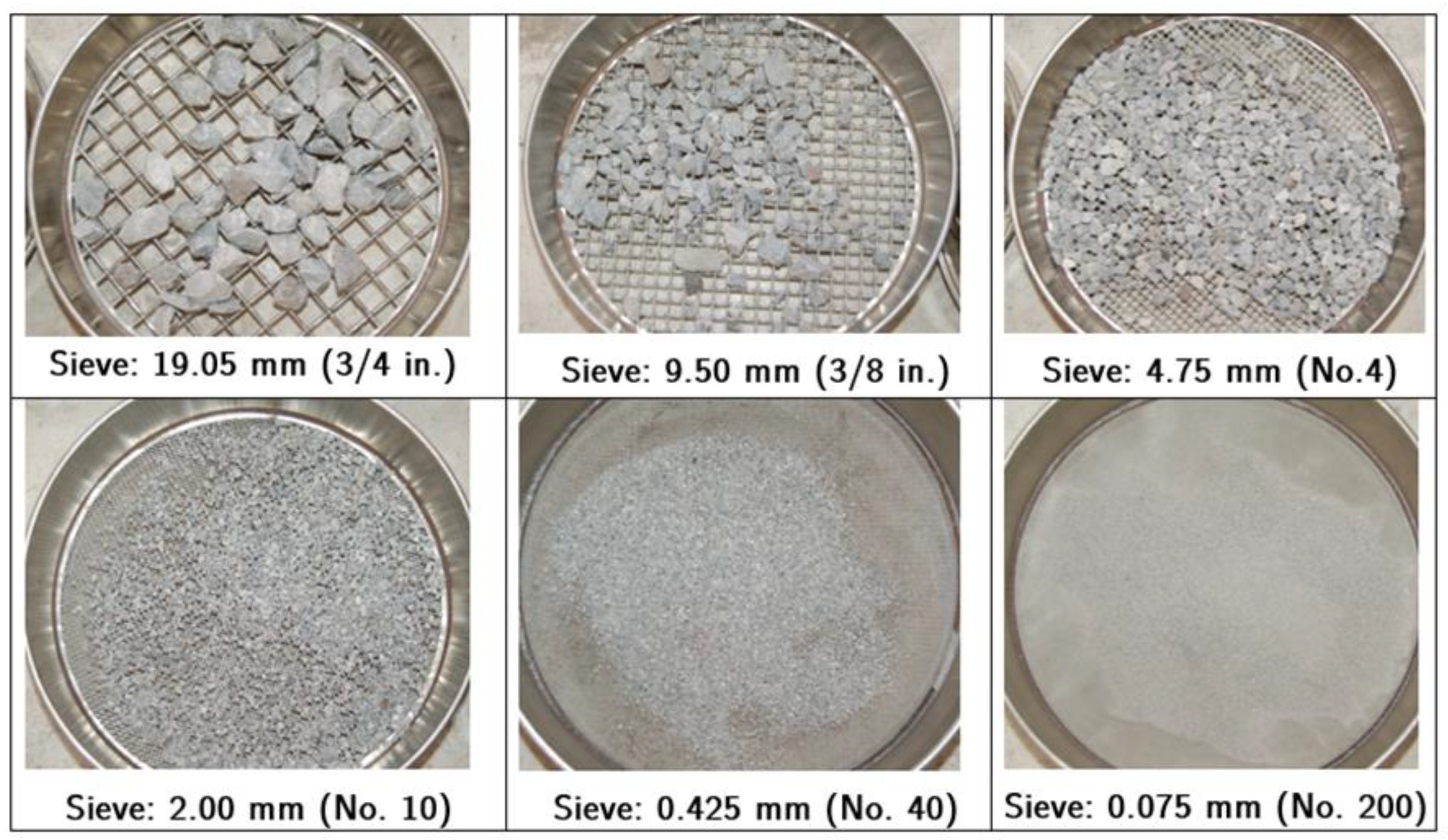
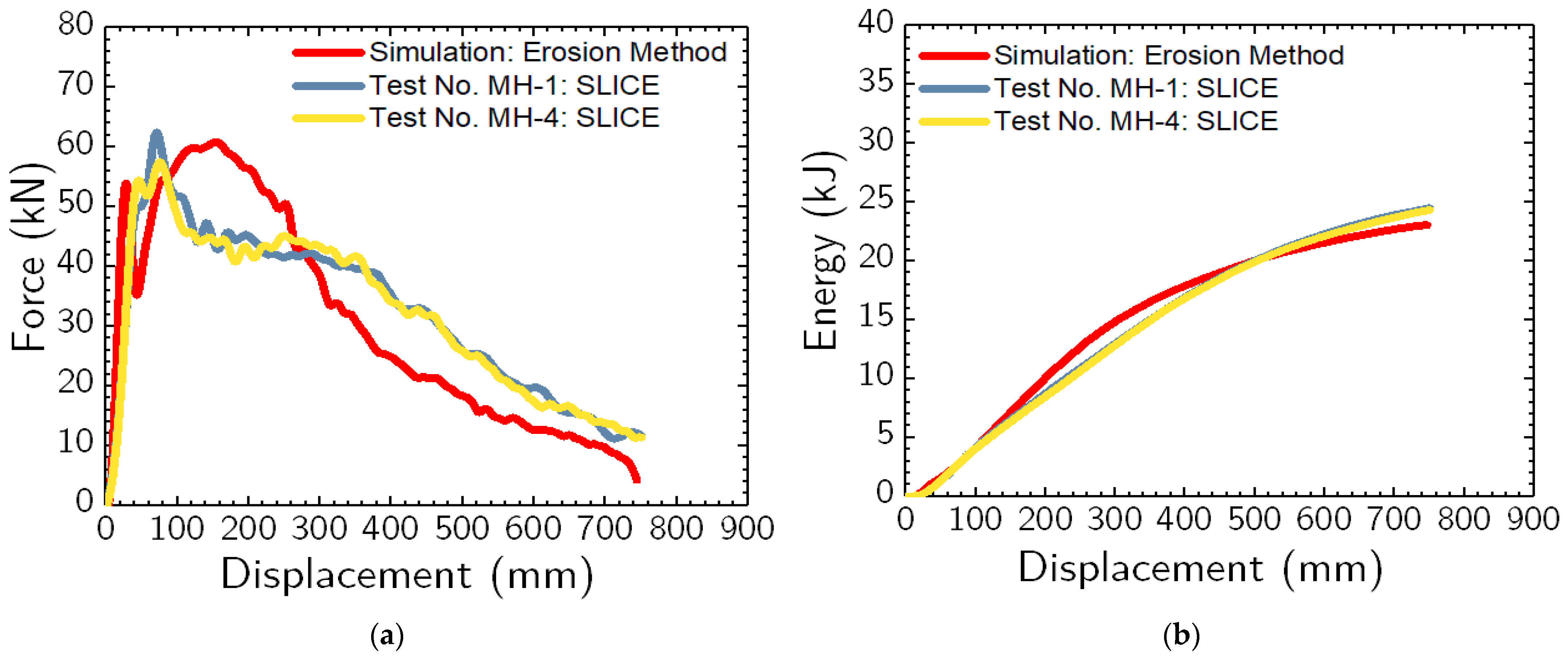
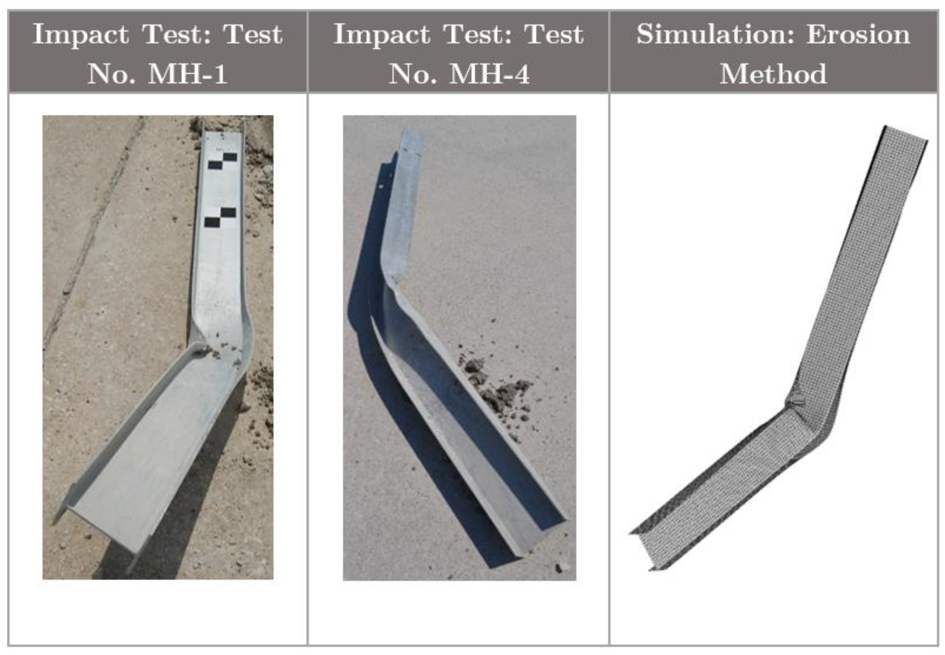
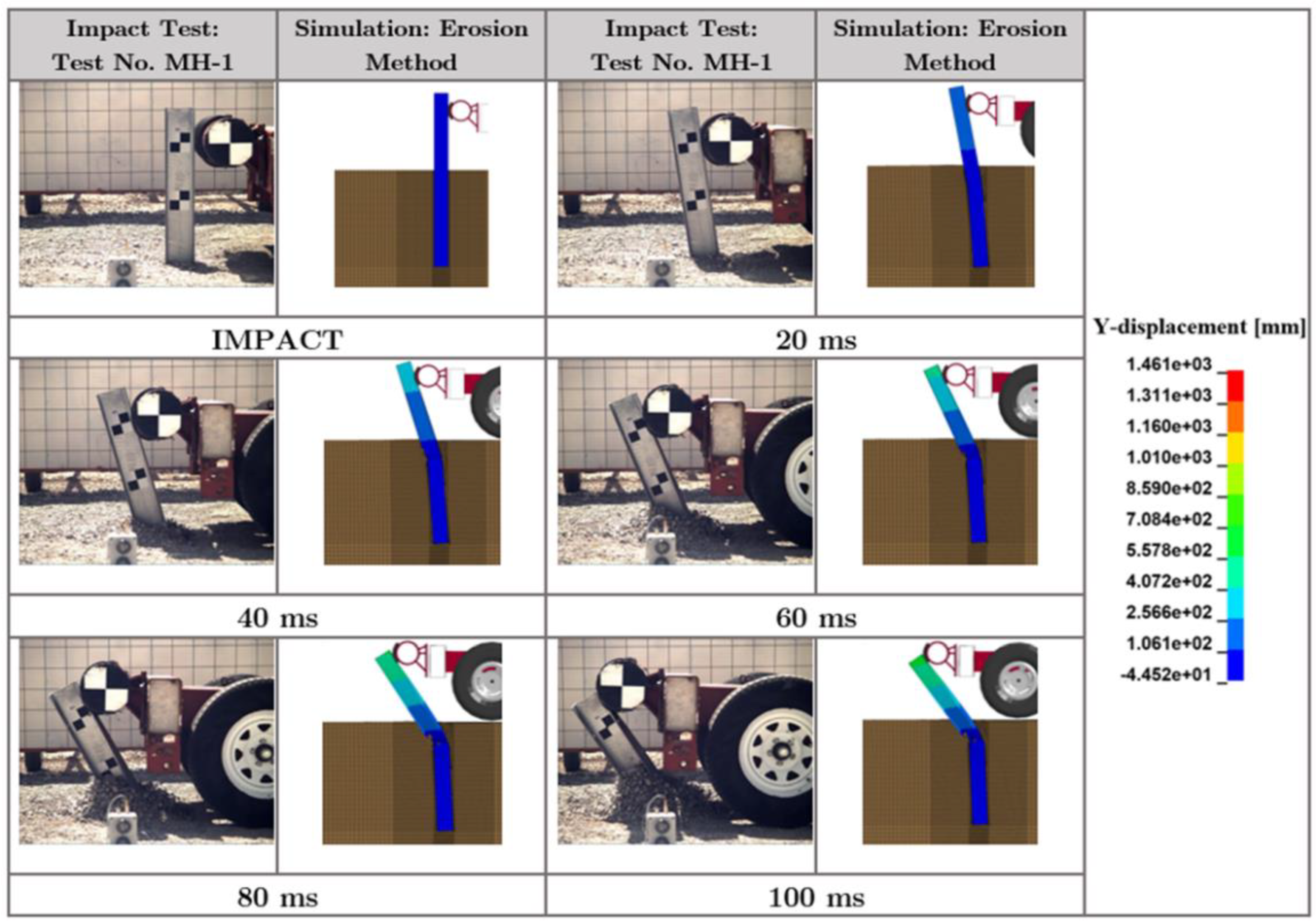
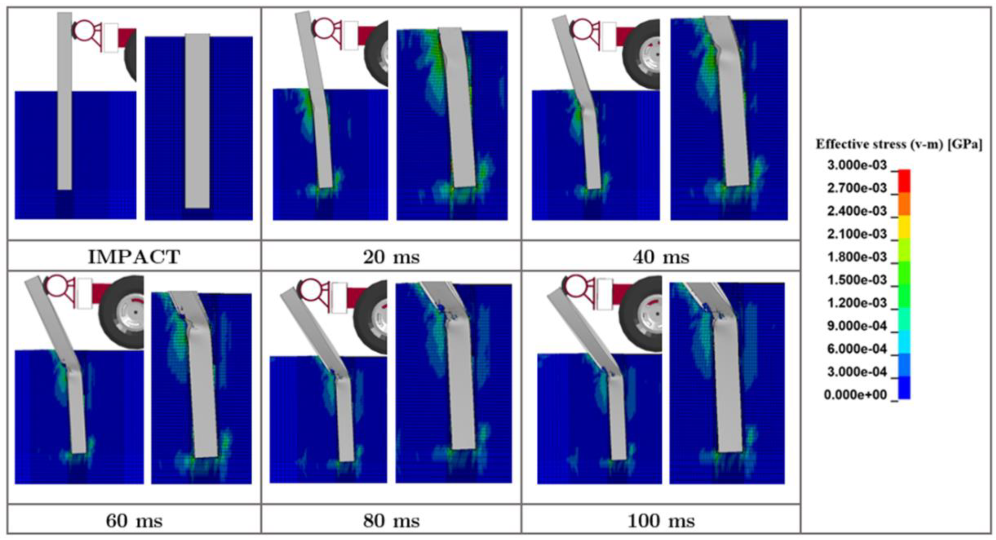
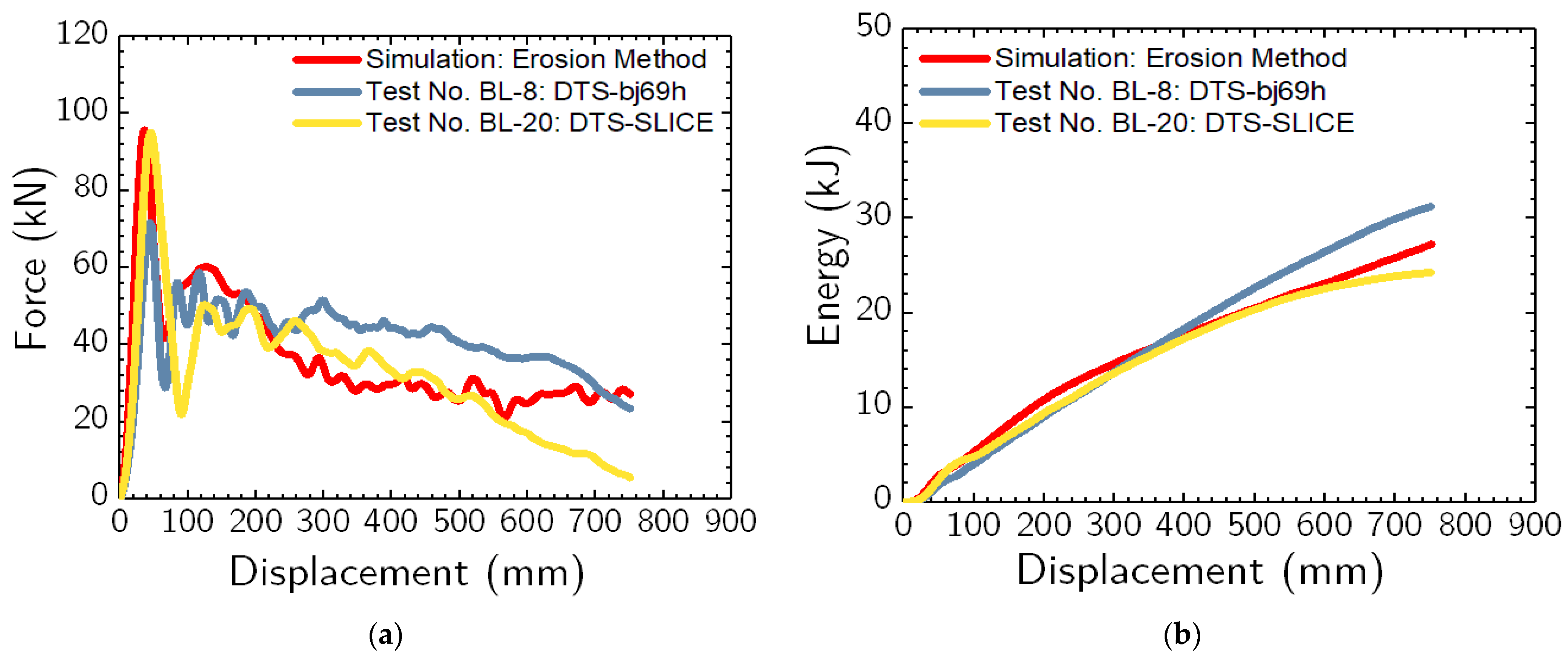
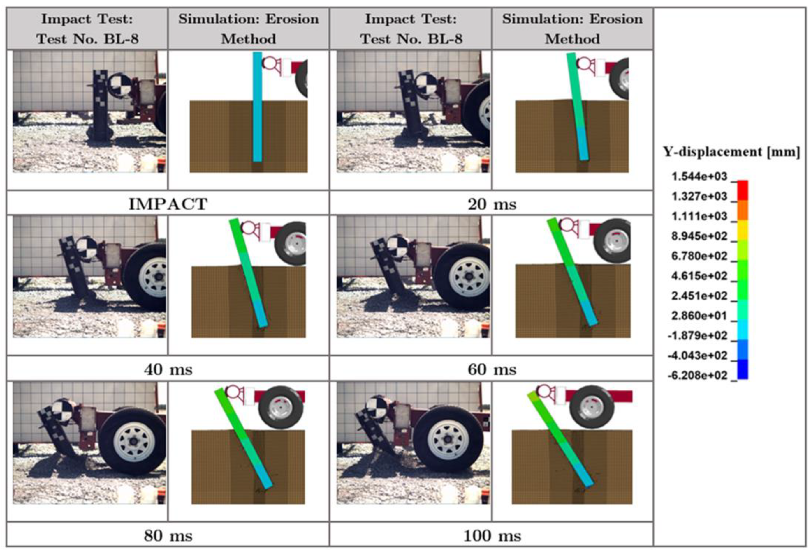
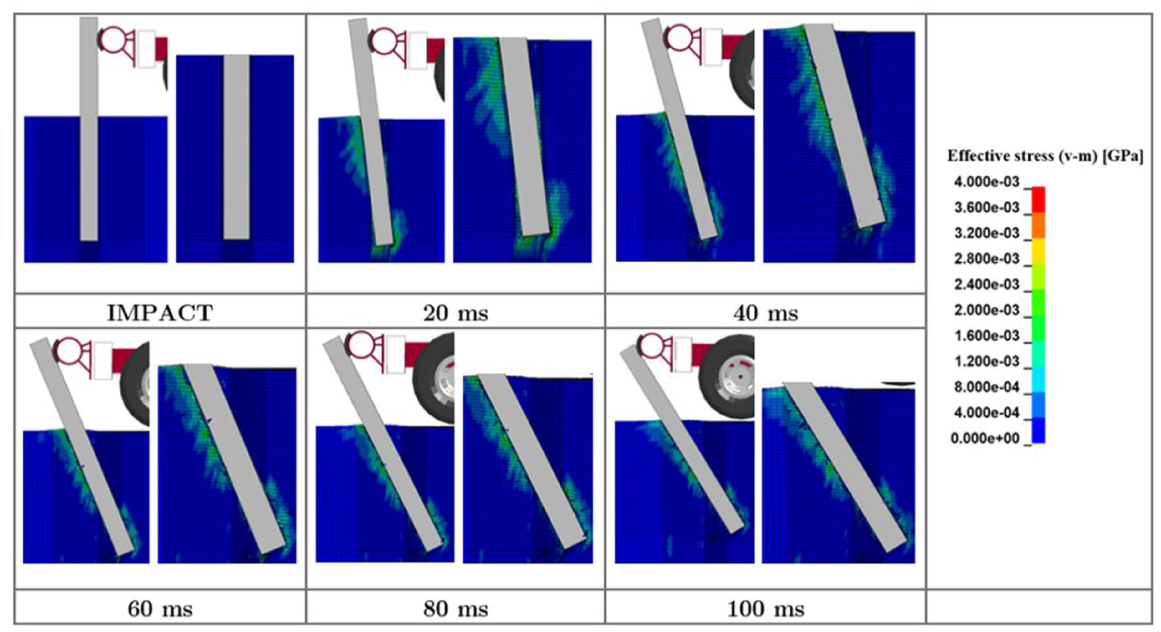
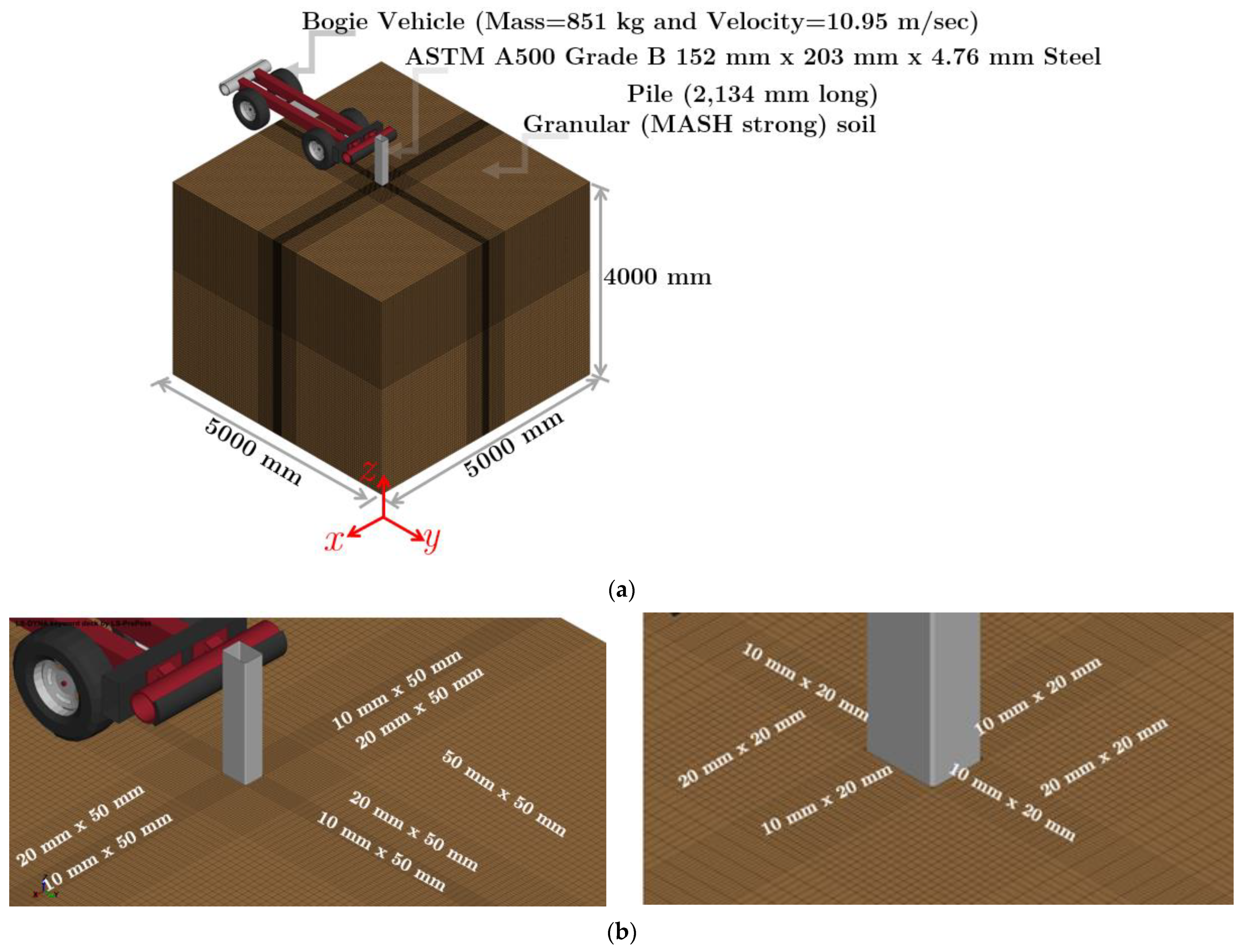
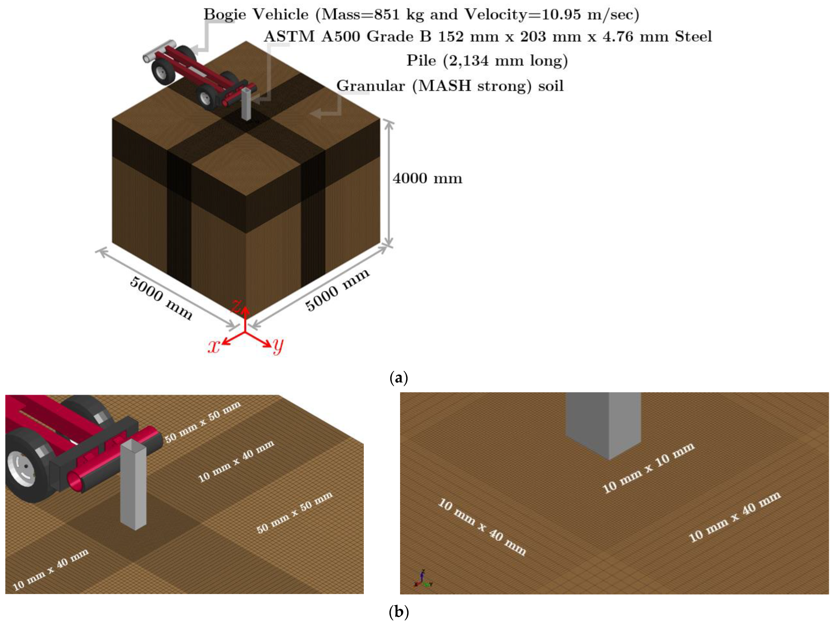
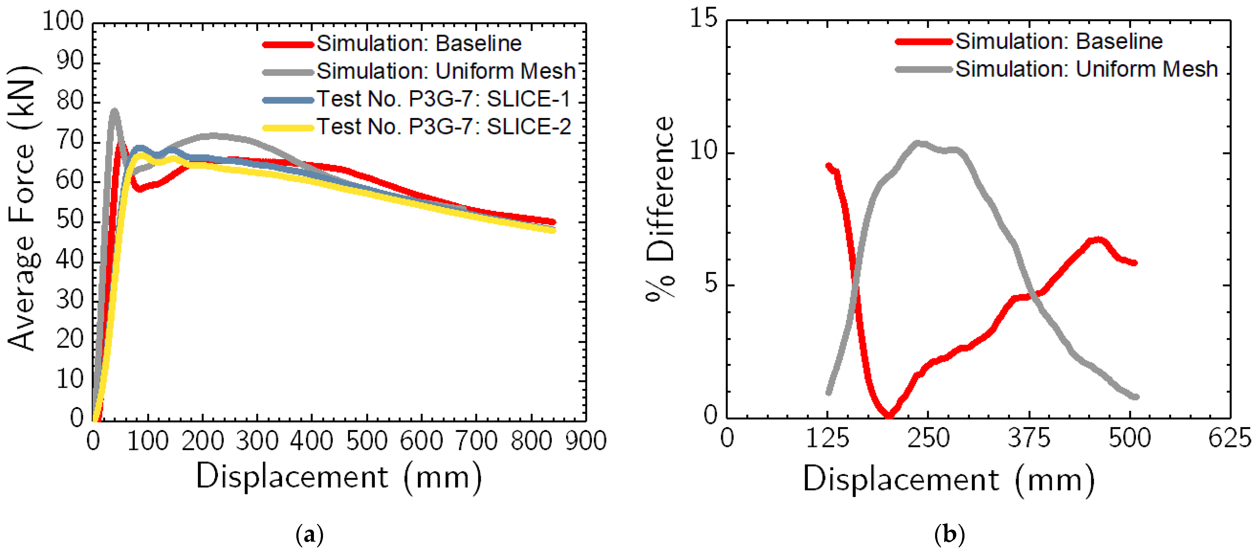
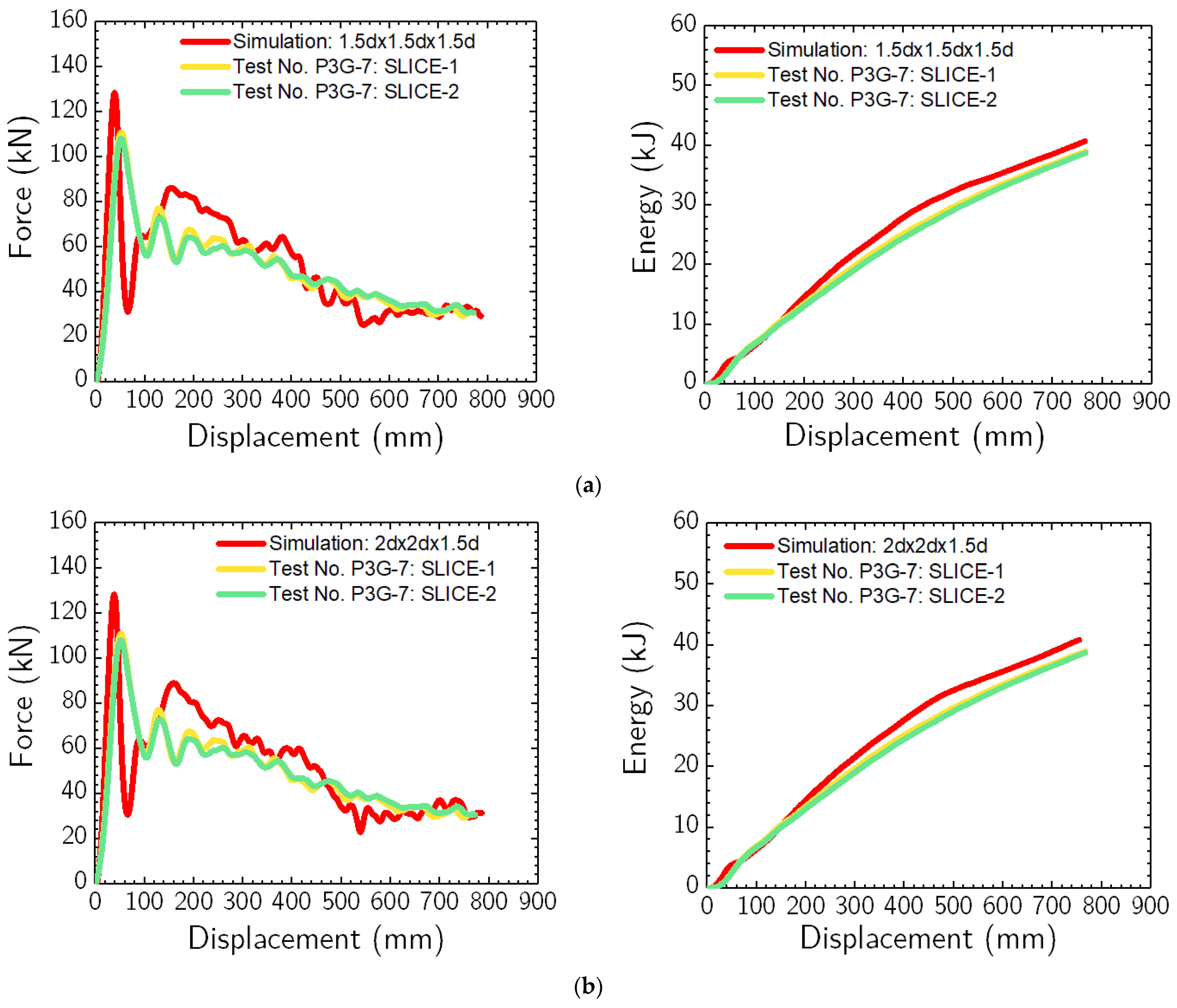
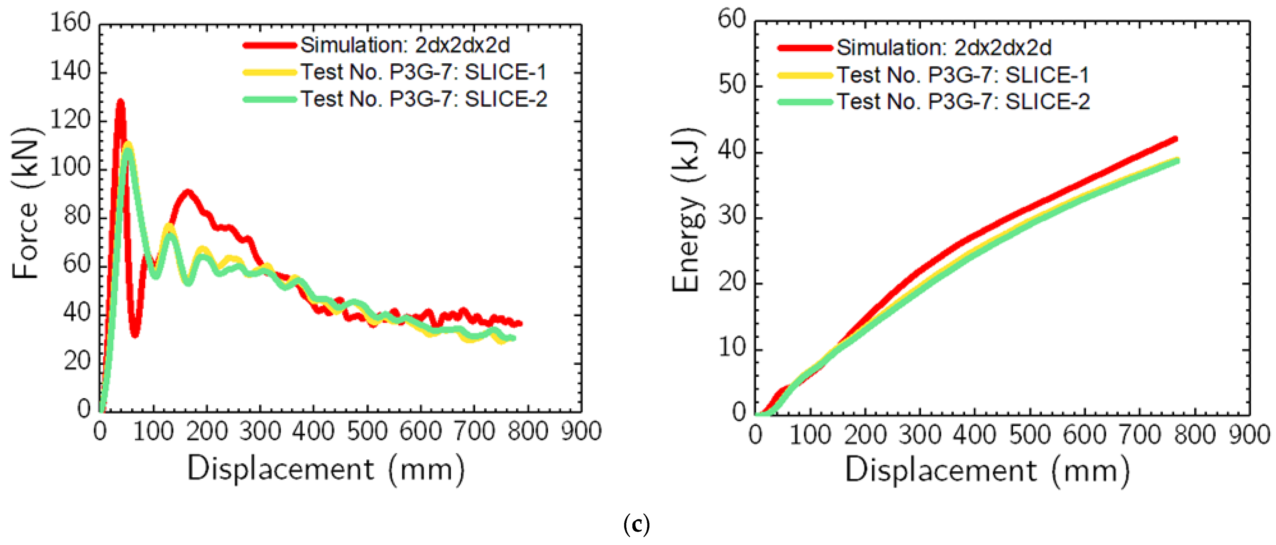
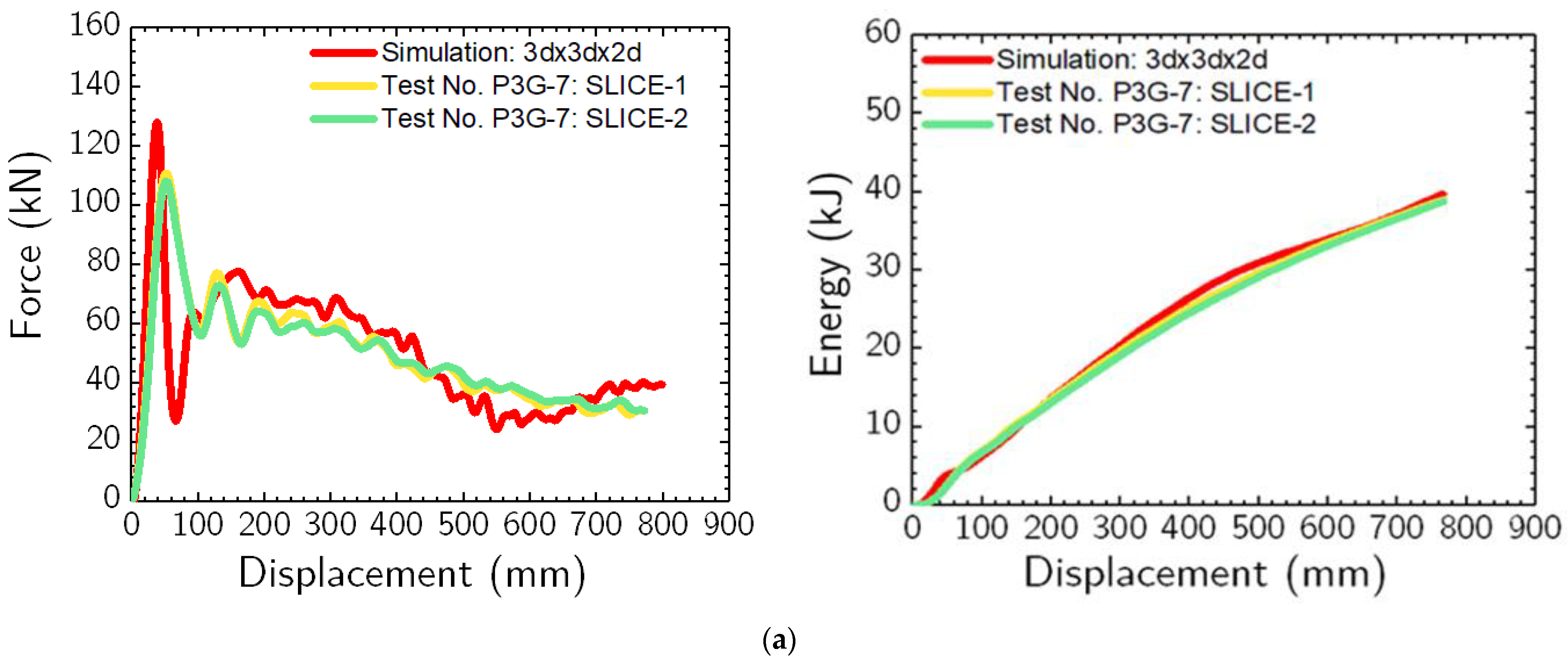
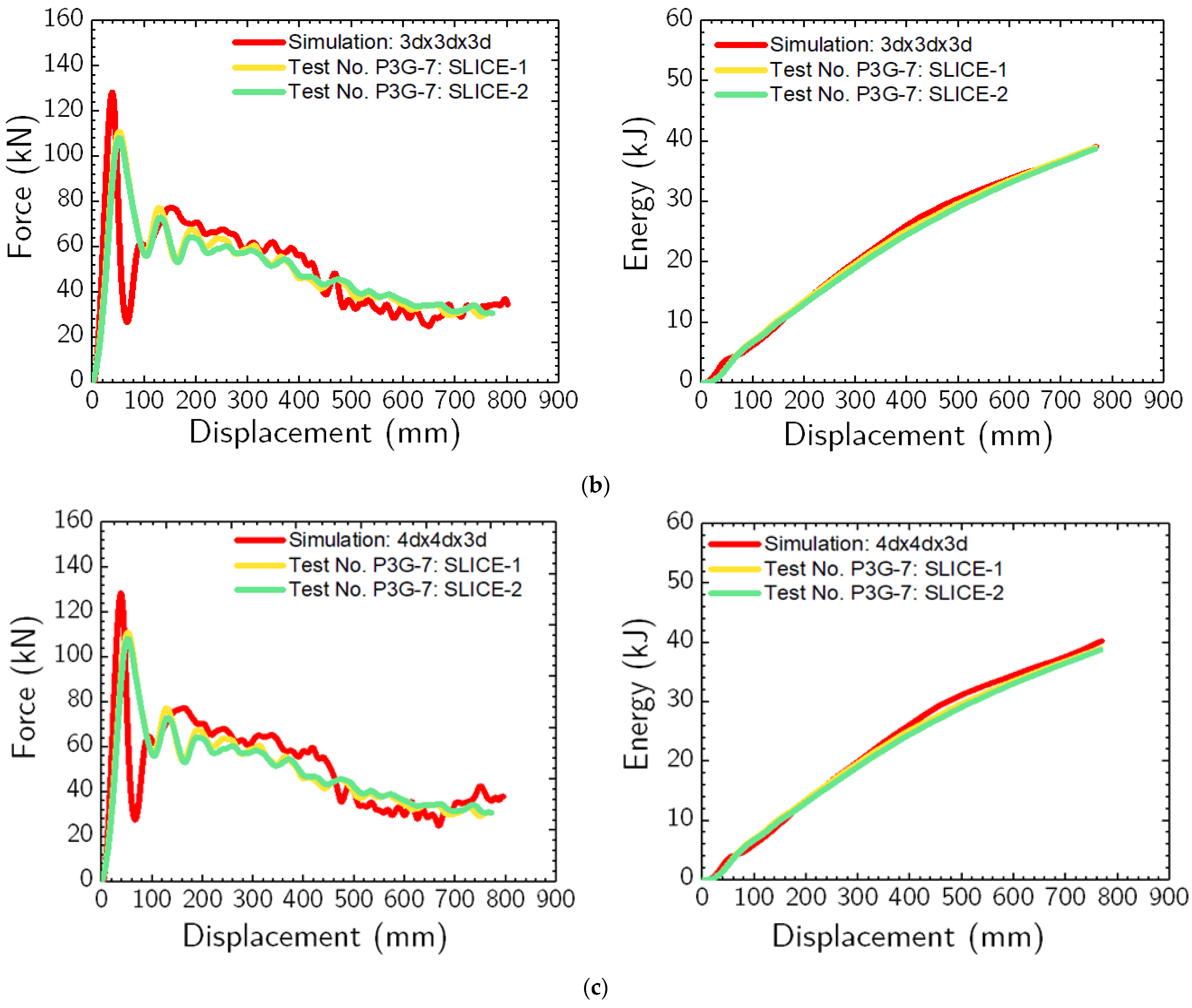
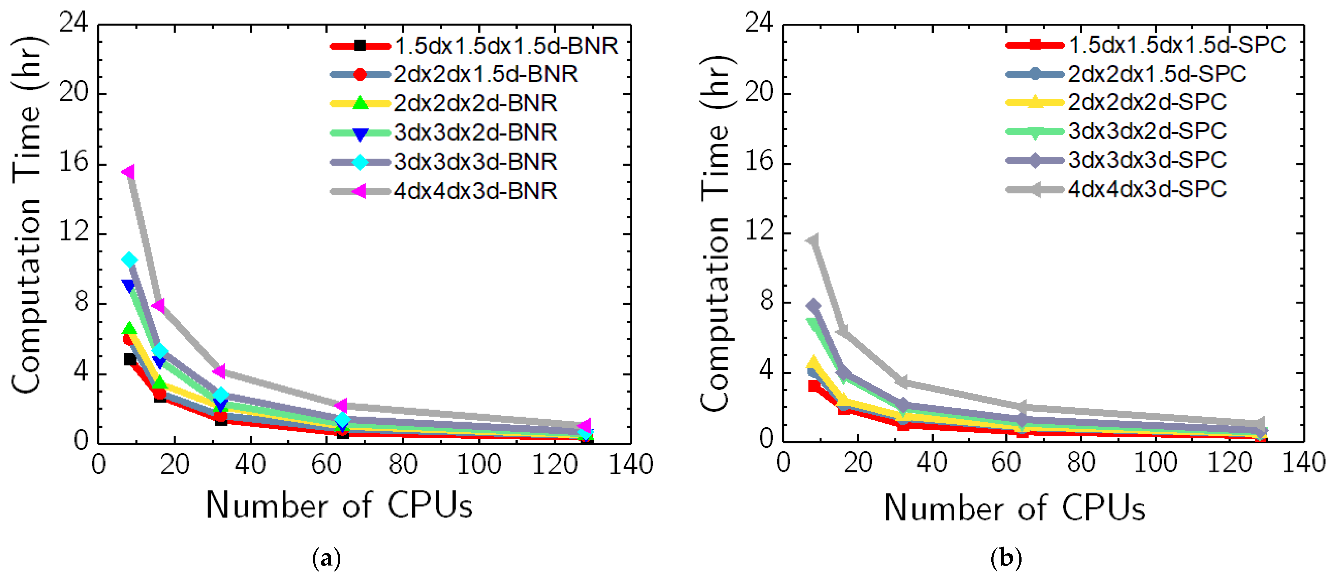
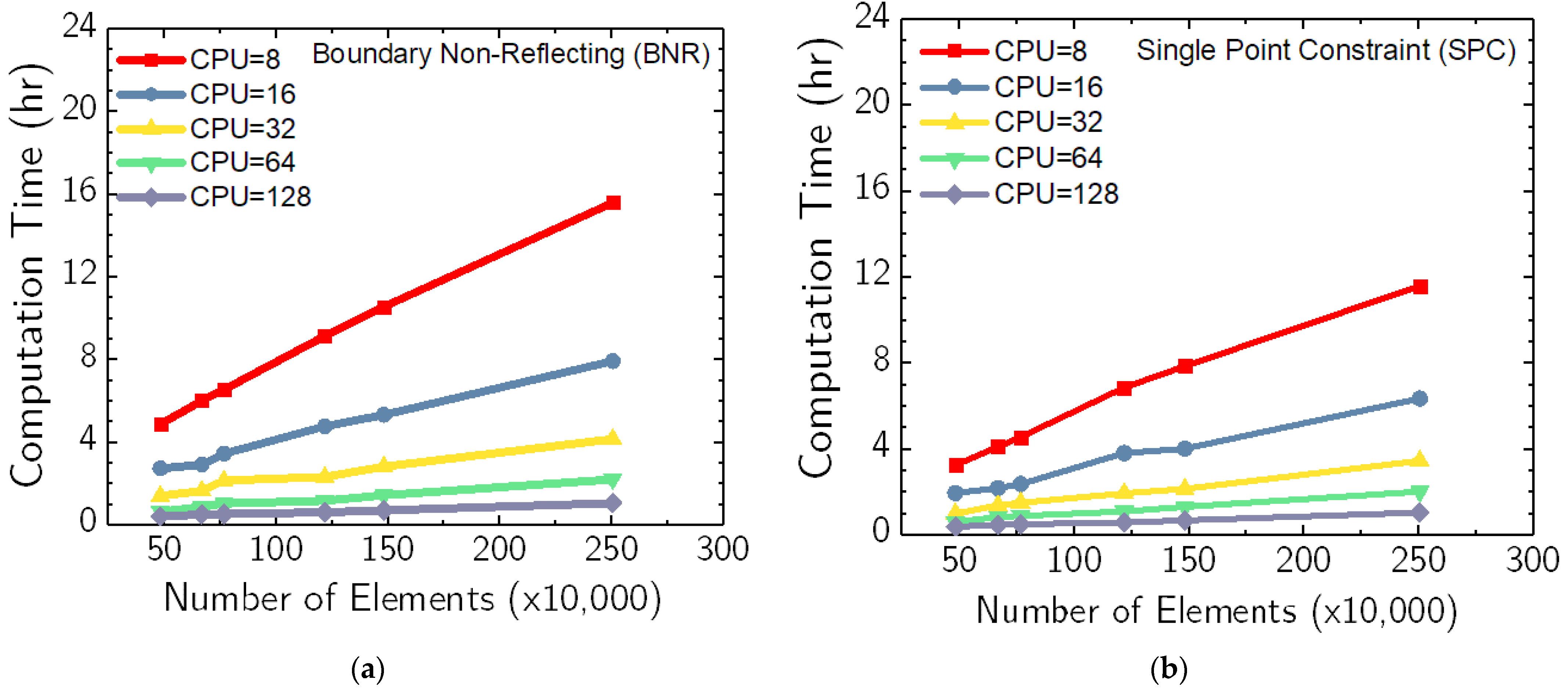